Analysis of Linear Predictive Coding

(1)

International Journal of Research (IJR)

e-ISSN: 2348-6848, p- ISSN: 2348-795X Volume 2, Issue 07, July 2015 Available at http://internationaljournalofresearch.org

Analysis of Linear Predictive Coding

Jennifer Jose & Smita Chopde

Department of Electronics and Telecommunication F.C.R.I.T Navi Mumbai, India

[email protected]

Department of Electronics and Telecommunication F.C.R.I.T Navi Mumbai, India

Abstract:

Linear predictive coding (LPC) is defined as a method for encoding an analog signal in which a particular value is predicted by a linear function of the past values of the signal. Human speech is produced in the vocal tract which can be approximated as a variable diameter tube. The linear predictive coding (LPC) model is based on a mathematical approximation of the vocal tract represented by this tube of a varying diameter. At a particular time, t, the speech sample s(t) is represented as a linear sum of the p previous samples. The most important aspect of LPC is the linear predictive filter which allows the value of the next sample to be determined by a linear combination of previous samples. This paper describes the quality of synthesized speech of a LPC model with varying the window shapes and window size.

Key Words: Linear Predictive Coding (LPC), voiced sounds, pitch, vocal tract

Introduction

Linear prediction is a signal processing technique that is used extensively in the analysis of speech signals. There are two types of voice coders: waveform-following coders and model-base coders. Waveform following coders will exactly reproduce the original speech signal if no quantization errors occur. Model based coders will never exactly reproduce the original speech signal, regardless of the presence of quantization errors, because they use a parametric model of speech production which involves encoding

and transmitting the parameters not the signal. Lpc Vocoders are considered model-based coders which mean that LPC coding is lossy even if no quantization errors occur.

The general algorithm for linear predictive coding involves an analysis or encoding part and a synthesis or decoding part. In the encoding, LPC takes the speech signal in blocks or frames of speech and determines the input signal and the coefficients of the filter that will be capable of reproducing the current block of speech. This information is quantized and transmitted. In the decoding, LPC rebuilds the filter based on the coefficients received. The filter can be thought of as a tube which, when given an input signal, attempts to output speech. Additional information about the original speech signal is used by the decoder to determine the input or excitation signal that is sent to the filter for synthesis. The particular source-filter model used in LPC is known as the Linear predictive coding model. It has two key components: analysis or encoding and synthesis or decoding.

(2)

International Journal of Research (IJR)

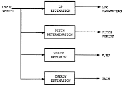
Figure 1 demonstrates parts of the LPC encoder receiver correspond to what parts in the human anatomy The analysis part of LPC involves examining the speech signal and breaking it down into segments or blocks. Each segment is than examined further to find the answers to several key questions:

 Is the segment voiced or unvoiced?  What is the pitch of the segment, if the

segment is voiced?

 What parameters are needed to build a filter that models the vocal tract for the current segment?

LPC analysis is usually conducted by a sender who answers these questions and usually transmits these answers onto a receiver. The receiver performs LPC synthesis by using the answers received to build a filter that when provided the correct input source will be able to accurately reproduce the original speech signal. Essentially, LPC synthesis tries to imitate human speech production.

Methodology

Input speech

First the input signal is sampled at a rate of 8Khz and 12Khz. The input signal is then broken up into segments or blocks which are each analysed and transmitted to the receiver.

Voiced /Unvoiced Determination

According to LPC-10 standards, before a speech segment is determined as being voiced or unvoiced it is first passed through a low-pass filter with a bandwidth of 1 kHz. Determining if a segment is voiced or unvoiced is important because voiced sounds have a different waveform than unvoiced sounds.

Figure 2: Voiced sound – Letter „e‟

Voiced sounds are usually vowels and can be considered as a pulse that is similar to periodic waveforms. These sounds have high average energy levels which means that they have very large amplitudes. Voiced sounds also have distinct resonant or formant frequencies.

Figure 3: Unvoiced sound – Letter „s‟

Unvoiced sounds are usually non-vowel or consonants sounds and often have very chaotic and random waveforms.

The following are the steps in the process of determining if a speech segment is voiced or unvoiced. The first step is to look at the amplitude of the signal, also known as the energy in the segment. If the amplitude levels are large then the segment is classified as voiced and if they are small then the segment is considered unvoiced. This determination requires a preconceived notion about the range of amplitude values and energy levels associated with the two types of sound [2].

Pitch Period Estimation

(3)

International Journal of Research (IJR)

air flow not vocal cord vibrations. It is very computationally intensive to determine the pitch period for a given segment of speech. There are several different types of algorithms that could be used [4]. One type of algorithm takes advantage of the fact that the autocorrelation of a period function,𝑅_𝑛(𝑘), will have a maximum when k is equivalent to the pitch period. These algorithms usually detect a maximum value by checking the autocorrelation value against a threshold value.

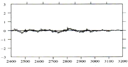
Figure 4 : Time-domain waveform of a short segment of voiced speech[3]

Figure 4 displays a time waveform for a short (40 ms) segment of a voiced sound. The x axis is the time scale, numbered in ms. The y axis is the amplitude of the recorded sound pressure. The high amplitude values mark the beginning of the pitch pulse. The first pitch period runs from near 0 ms to about 10 ms, the second from near 10 ms to about 20 ms.

Determination of the Gain

Gain should be determined by matching the energy in the signal with the energy of the linear predicted samples[6].The gain can be expressed as

𝐺2_{= 𝑅𝑛 (0)-}𝑝 _𝛼𝑘 𝑘=1 𝑅𝑛 (𝑘)

Where 𝑅𝑛 (𝑘) is the auto-correlation function and p is the predictor coefficients

LPC Synthesis

Figure 5 : Block Diagram of simplified model for speech production[5]

Figure 5 shows an implementation of the source filter speech production model. The pulse generator produces a periodic waveform at intervals of the pitch period. The noise generator outputs a random sequence of white (equal power across the spectrum) noise. The voicing information controls the switch that decides whether to select the periodic (voiced) or random (unvoiced) excitation signal. The excitation signal is then frequency shaped by the LPC filter and multiplied by the gain to produce the correct energy (signal amplitude) of the output synthesized speech.

Implementation and test results

The implementation was carried out in MATLAB software. The sampled speech signal was divided into frames using a hamming window. The pitch estimation was carried out by the method of autocorrelation. The following are the results obtained from MATLAB for vowels and sentences of a female speaker.

(4)

International Journal of Research (IJR)

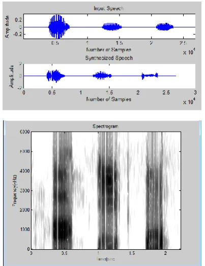
Figure 7 : Plot of /aa-ee-uu/ sampled at the rate 12Khz.with thiry predictor coefficients

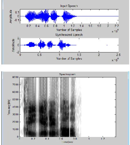
Figure 8 : Plot of a sentence “/a year ago/ “sampled at the rate 12Khz.with thiry predictor coefficients

Figure 9 : Plot of a sentence “/a year ago/ “sampled at the rate 12Khz.with ten predictor coefficients

A comparison of the original speech sentences against the LPC reconstructed speech was studied. The reconstruction was carried out using ten and thirty predictor Coefficients. The reconstructed signals sound mechanized and noisy. In case of vowels with a sampling frequency of 12Khz and ten predictor coefficients the reconstructed signal is intelligible but in case of sentences sampled at a rate of 12Khz and ten predictor coefficients made the speech signal very noisy but increasing the predictor coefficients to thirty predictor coefficients reduced the noise and made it more intelligible. The LPC reconstructed speech sounds guttural with a lower pitch than the original sound. The sound seems to be whispered. The noisy feeling is very strong.

REFERENCES

[1.] D. O‟Shaughnessy, Speech Communication- Human and Machine. Reading, MA: Addison-Wesley, 1987.

[2.] M.H Johnson, Speech Coding: Fundamentals and Applications Wiley Encyclopedia of

(5)

International Journal of Research (IJR)

[3.] A. S. Spanias, “Speech Coding: A Tutorial Review” Proc. IEEE. VOL.82, October 1994 Tavel, P. 2007 Modeling and Simulation Design. AK Peters Ltd.

[4.] Simon Haykin “ Communication systems” Wiley India.

[5.] C.Xydeas.“An Overview Of Speech Coding

Techniques” IEEE Trans Vol No. 3, June 1981.

[6.] L. R. Rabiner and R. W. Schafer, Digital Processing of Speech Signals. Englewood Cliffs,NJ:

Prentice-Hall, 1978.