Automatic Assessment of Cardiac Left Ventricular Function Via Magnetic Resonance Images

(1)

Western University Western University

Scholarship@Western

Electronic Thesis and Dissertation Repository

12-17-2012 12:00 AM

Automatic Assessment of Cardiac Left Ventricular Function Via

Magnetic Resonance Images

Mariam Afshin

The University of Western Ontario

Supervisor Terry Peters

The University of Western Ontario Joint Supervisor Shuo Li

The University of Western Ontario

Graduate Program in Biomedical Engineering

A thesis submitted in partial fulfillment of the requirements for the degree in Doctor of Philosophy

Follow this and additional works at: https://ir.lib.uwo.ca/etd

Part of the Biomedical Engineering and Bioengineering Commons

Recommended Citation Recommended Citation

Afshin, Mariam, "Automatic Assessment of Cardiac Left Ventricular Function Via Magnetic Resonance Images" (2012). Electronic Thesis and Dissertation Repository. 1035.

https://ir.lib.uwo.ca/etd/1035

This Dissertation/Thesis is brought to you for free and open access by Scholarship@Western. It has been accepted for inclusion in Electronic Thesis and Dissertation Repository by an authorized administrator of

(2)

AUTOMATIC ASSESSMENT OF CARDIAC LEFT VENTRICULAR

FUNCTION VIA MAGNETIC RESONANCE IMAGES

(Thesis format: Integrated Article)

by

Mariam Afshin

Graduate Program in Biomedical Engineering

Submitted in partial fulfillment

of the requirements for the degree of

Doctorate of Philosophy

The School of Graduate and Postdoctoral Studies

Western University

London, Ontario, Canada

c

(3)

WESTERN UNIVERSITY

School of Graduate and Postdoctoral Studies

CERTIFICATE OF EXAMINATION

Supervisors:

. . . . Drs. T. M. Peters and S. Li

Supervisory Committee:

. . . . Dr. Grace Parraga

. . . . Dr. Gerard M. Guiraudon

Examiners:

. . . . Dr. Aaron Fenster

. . . . Dr. James Johnson

. . . . Dr. Michael Chu

. . . . Dr. Kaleem Siddiqi

The thesis by

Mariam Afshin

entitled:

AUTOMATIC ASSESSMENT OF CARDIAC LEFT VENTRICULAR FUNCTION VIA MAGNETIC RESONANCE IMAGES

is accepted in partial fulfillment of the requirements for the degree of

Doctorate of Philosophy

. . . . Date

. . . .

(4)

Abstract

Automating global and segmental (regional) assessments of cardiac Left Ventricle (LV)

function in Magnetic Resonance Images (MRI) has recently sparked an impressive research

ef-fort, which has resulted a number of techniques delivering promising performances. However,

despite such an effort, the problem is still acknowledged to be challenging, with substantial

room for improvements in regard to accuracy. Furthermore, most of the existing techniques are

labour intensive, requiring delineations of the endo- and/or epi-cardial boundaries in all frames

of a cardiac sequence.

On the one hand, global assessments of LV function focus on estimation of the Ejection

Fraction (EF), which quantifies how much blood the heart is pumping within each beat. On the

other hand, regional assessments focus on comprehensive analysis of the wall motions within

each of the standardized segments of the myocardium, the muscle which contracts and sends

the blood out of the LV.

In clinical practice, the EF is often estimated via manual segmentation of several images in a

cardiac sequence which is prohibitively time consuming, or via automatic segmentation, which

is a challenging and computationally expensive task that may result in high estimation errors.

Additionally, the diagnosis of the segmental dysfunction is based on visual LV assessment,

which is subject to high inter-observer variability.

In this thesis, we propose accurate methods to estimate both global and regional LV

func-tion with minimal user inputs in real-time from statistics estimated in MRI. From a simple user

input, we build image statistics for all the images in a subject dataset. We demonstrate that

these statistics are correlated with regional as well as global LV function. Different machine

learning techniques have been employed to find these correlations. The regional dysfunction is

investigated in terms of a binary/multi-classification problem.

A comprehensive evaluation over 20 subjects demonstrated that the estimated EFs

corre-lated very well with those obtained from independent manual segmentations. Furthermore,

(5)

pro-posed method yielded a very competitive performance. For regional binary classification, we

report a comprehensive experimental evaluation of the proposed algorithm over 928 cardiac

segments obtained from 58 subjects. Compared against ground-truth evaluations by

experi-enced radiologists, the proposed algorithm performed competitively, with an overall

classifi-cation accuracy of 86.09% and a kappa measure of 0.73. We also report a comprehensive

experimental evaluation of the proposed multi-classification algorithm over the same dataset.

Compared against ground-truth labels assessed by experienced radiologists, the proposed

(6)

Keywords: left ventricle (LV), ejection fraction (EF), bhattacharyya coefficient, machine

learning, artificial neural network (ANN), magnetic resonance images (MRI), principal

com-ponent analysis (PCA), kernel density estimation (KDE), regional wall motion abnormality

detection, image statistics, linear discriminant analysis (LDA), linear support vector machine

(7)

Acknowlegements

I owe this success to a number of people without whom none of this would have been

possible.

I would like to express my sincere thanks to my supervisors Dr. Terry Peters and Dr. Shuo

Li for all their help and encouragements throughout my program. I would like to thank Dr.

Peters for giving me the opportunity to be part of his group and supporting me during last

four years. I also, would like to thank Dr. Shuo Li for giving me the opportunity to join

Biomedical Engineering program at Western, believing in me and pushing me to achieve goals

that I sometimes considered unachievable.

Special thanks to Dr. Ismail Ben Ayed whose expertise was crucial to my success. I thank

Ismail for inspiring and challenging me, and for sharing his research insight and passion with

me during my Ph.D. I thank Dr. Kumaradevan Punithakumar and Dr. Max Law for sharing

their vast technical knowledge and experience with me.

I would like to thank my advisory committee members, Dr. Grace Parraga and Dr. Gerard

Guiraudon for their continuous support and positive feedbacks. During my advisory meetings,

they motivated me to learn and overcome the technical challenges.

I would like to thank all the lab members in Dr Peters’ group as well as members in Digital

Imaging Group of London. Also, thanks to my wonderful friends for their help.

Last, but not least, special thanks to my family especially my father, my mother, my brother,

my sister and my nephews, Hossein and Kamyar, for their unconditional love and support in

every step of my life. Thanks for encouraging me to follow my dreams. Huge thanks to my

boyfriend Pouyan whose love is the reason I start everyday with a smile. Thanks for your

(8)

List of Figures

1.1 Blood Circulation. The figure is adopted from:

http://en.wikipedia.org/wiki/Circulatory_system . . . 4

1.2 AHA standard for LV regional segments. . . 17

2.1 User input: (a) frame 1 (slices 1,7, and 10); (b)Γ_in (the blue curve within the

cavity) andΓ_out (the red curve enclosing the cavity) are given by the user in the

reference image (the middle image). Γ_in is used solely in the reference image

to compute PRΓ_in,I, whereasΓout is superimposed systematically (without

addi-tional user effort) to all the other images (refer to Figs. 2.2 and 2.3) to compute

PRΓout,Ii,j. . . 40

2.2 Superimposing red curve in End-systole: frame 7 (slices 1,7, and 10): Γ_out is

superimposed systematically (without additional user effort) to all the slices in

the 7th frame. . . 40

2.3 Superimposing red curve in End-diastole: frame 20 (slices 1,7, and 10):Γ_outis

superimposed systematically (without additional user effort) to all the slices in

(14)

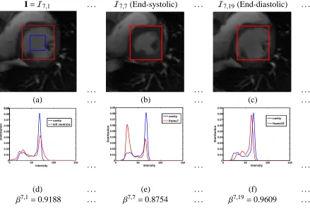
2.4 Computing image statistics for the frames of slice 7 (middle slice): (a)

refer-ence image (red curve: Γout, blue curve: Γin); (b): frame 7 (end-systolic) and

(c) frame 19 (end-diastolic); (d), (e), and (f) the corresponding intensity

distri-butions and Bhattacharyya measures (βi j_{). We observe that the variations of}_βi j

are similar to the variations of the LV cavity areas. For instance at the end of

systole (the middle column), the smallest cavity area coincides with the lowest

Bhattacharyya measure. . . 43

2.5 Computing image statistics for the frames of slice 1 (apical slice): (a) frame 1

(the red curve,Γ_out, is superimposed systematically to all the images without

additional user effort); (b): frame 7 and (c) frame 19; (d), (e), and (f) the

corre-sponding intensity distributions and Bhattacharyya measures (βi j). Again, we

observe that the variations ofβi j are similar to the variations of the LV cavity

areas. . . 44

2.6 Computing image statistics for all the images of slice 10 (basal slice): (a) frame

1; (b) frame 7 and (c) frame 19; (d), (e), and (f) the corresponding intensity

distributions and Bhattacharyya measures (βi j). . . 45

2.7 A sample example which shows the variations of the LV cavity areas of apical

slice obtained from manual segmentations. . . 52

2.8 A sample example which shows the variations of the Bhattacharyya image

statistics of apical slice. We observe that these statistics are non-linearly

re-lated to the manually obtained LV cavity areas depicted in Fig. 2.7. . . 53

2.9 A sample example which shows the variations of the LV cavity areas of a

mid-cavity slice obtained from manual segmentations. . . 53

2.10 A sample example which shows the variations of the Bhattacharyya image

statistics of a midcavity slice. We observe that these statistics are non-linearly

(15)

2.11 A sample example which shows the variations of the LV cavity areas of basal

slice obtained from manual segmentations. . . 54

2.12 A sample example which shows the variations of the Bhattacharyya image statistics of basal slice. We observe that these statistics are non-linearly related to the manually obtained LV cavity areas depicted in Fig. 2.11. . . 55

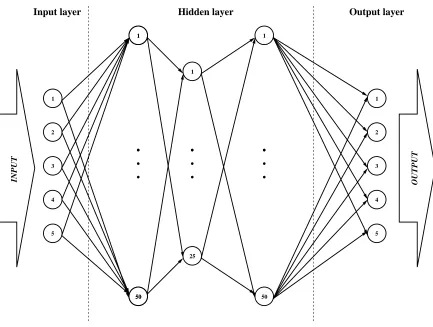
2.13 The ANN consists of one input layer, three hidden layers, and one output layer. 56 2.14 The training phase. . . 56

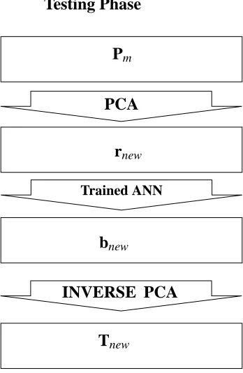
2.15 The testing phase: the estimated Bhattacharyya statistics are fed to the network and the corresponding LV cavity areas are predicted. . . 57

2.16 Variation of the volume of the LV cavity in each heart beat. . . 58

2.17 Automatic versus manual cavity areas. . . 60

2.18 Automatic versus manual cavity volumes. . . 60

2.19 Automatic and manual EFs in 20 subjects. . . 61

2.20 Errors (20 subjects) obtained with the proposed automatic method (red curve), the graph-cut segmentation (blue curve), and the level-set segmentation (green curve). The proposed method yielded a much lower curve and, therefore, a significant improvement in accuracy. . . 63

2.21 Mean error as a function of the number of most significant eigenvectors. . . 64

2.22 Mean error as a function of the number of neurons in the first hidden layer. . . . 65

2.23 Mean error as a function of the number of neurons in the second hidden layer. . 65

2.24 Mean error as a function of the number of neurons in the third hidden layer. . . 66

2.25 Mean error as a function of the size of the user-provided region of interest. . . . 66

2.26 Automatic versus manual cavity areas for an apical slice of a single subject. . . 67

2.27 Automatic versus manual cavity areas for a mid-cavity slice of a single subject. 67 2.28 Automatic versus manual cavity areas for a basal slice of a single subject. . . . 68

2.29 Automatic versus manual cavity volumes: the best case in the 20 subjects. . . . 68

(16)

2.31 Automatic versus manual cavity volumes: the worst case in the 20 subjects. . . 69

3.1 User-provided delineation in one single frame (reference image Is) for three representative slices: (a) apical, (b) mid-cavity and (c). . . 76

3.2 The regional segments superimposed on reference image Is. . . 76

3.3 A simple synthetic example which demonstrates how some segmentation-free image statistics correlate with the dynamics of a moving region. The larger circle is a fixed region while the size of the smaller circle varies. The smaller circle illustrates the cavity motion. . . 79

3.4 (a): Manual segmentation of the reference (end-diastolic) frame. (b): Regional segments of the reference frame. (c-d): regional segments of the reference frame superimposed systematically (without additional user effort) onto the rest of the frames. . . 80

3.5 (a) Reference image Is; (b) Endo and epi-cardial boundaries in Is; (c) boundary of regional segment i in the reference frame. . . 81

3.6 (a-c): Regional myocardial segments of an apical slice superimposed on sub-sequent frames. (d-f): The corresponding image statistics. . . 81

3.7 (a-c): Regional myocardial segments of a mid-cavity slice superimposed on subsequent frames. (d-f): The corresponding image statistics. . . 82

3.8 (a-c): Regional myocardial segments of a basal slice superimposed on subse-quent frames. (d-f): The corresponding image statistics. . . 82

3.9 The procedure of estimating the statistical image-based features. . . 84

3.10 Overview of the training phase. . . 87

3.11 Overview of the testing phase. . . 89

3.12 User input to specify initial segmentation and anatomical landmarks on the first frame. . . 90

3.13 Projected apical features (β~i mp) obtained following the LDA transformation. . . 92

(17)

3.15 Projected basal features (β~i

mp) obtained following the LDA transformation. . . . 94

3.16 Decision boundaries and support vectors for the apical segments. . . 95

3.17 Decision boundaries and support vectors for the mid-cavity segments. . . 96

3.18 Decision boundaries and support vectors for the basal segments. . . 97

3.19 ROCs for apical segments: The closer the curve to the left-hand top corner, the

better the classification performance. . . 98

3.20 ROCs for mid-cavity segments: The closer the curve to the left-hand top corner,

the better the classification performance. . . 98

3.21 ROCs for basal segments: The closer the curve to the left-hand top corner, the

better the classification performance. . . 99

4.1 Identifying 16 regional segments in the reference frame. (a): user-provided

segmentation of the reference frame. (b): 16 regional segments of the

ref-erence frame. (c-d): regional segments of the refref-erence frame superimposed

systematically to the rest of the frames. . . 111

4.2 (a-c): mid-cavity regional segments superimposed on subsequent frames.

(d-f): the similarity measures between the cavity region in the first frame and the

regional segments in all other frames. (g-i): the similarity measures between

the myocardium region in the first frame and regional segments in all other

frames. . . 112

4.3 User input to specify initial segmentation and anatomical landmarks on the first

frame. . . 113

4.4 Accuracy(%) for each of the 16 regional segments. The average accuracy over

all 16 segments is equal to 74.14%. . . 116

4.5 Bull’s eye plot obtained from ground-truth in column 1,3. The colors depict

the four classes: red for normal, green for hypokinetic, yellow for akinetic and

(18)

List of Tables

2.1 Statistical measures of the conformity between automatically and manually

computed areas and volumes. . . 61

2.2 Statistical measures of the conformity between automatically and manually

computed EFs. . . 62

2.3 Errors (std and mean) and computation time (in seconds) with the proposed

method and with graph-cut and level-set estimation of the EF based on the

recent segmentation algorithms in [2,3]. . . 62

3.1 Details of the datasets used in the evaluation of the proposed method. . . 90

3.2 The AUCs corresponding to Figs. 3.19, 3.20, 3.21 and the corresponding

Bhat-tacharyya distance metrics (_B) of normal/abnormal distributions. The higher

the values, the more discriminative the ability of the classifier. . . 96

3.3 Classification accuracy using a leave-one-third-of-the-subjects-out approach.

The proposed method achieved an overall classification accuracy of 86.09%. . . 100

3.4 Comparisons between the proposed method and visual assessment scoring by

experienced radiologists. The proposed method yielded a kappa measure of

0.73, a substantial agreement with radiologists’ results. . . 100

3.5 Comparisons of the proposed method with recent existing methods of regional

myocardial abnormality detection. All the existing methods require either

man-ual or automatic (registration-based) segmentations of several frames in a

(19)

(20)

List of Abbreviations

2D Two-Dimensional

3D Three-Dimensional

HF Heart Failure

LV Left Ventricle

RV Right Ventricle

LA Left Atrium

RA Right Atrium

MRI Magnetic Resonance Imaging

CMR Cardiac Magnetic Resonance

RF Radio Frequency

MR Magnetic Resonance

SSFP Steady-State Free Precession

CT Computed Tomography

EF Ejection Fraction

AHA American Heart Association

IHD Ischemic Heart Disease

LVEF Left ventricular Ejection Fraction

GMM Gaussian Mixture Model

ROI Region Of Interest

(21)

PDF Probability Density Function

PCA Principal Component Analysis

AAM Active Appearance Models

ANN Artificial Neural Network

HMM Hidden Markov Model

SDE Shannons Differential Entropy

ICA Independent Component Analysis

LDA Linear Discriminant Analysis

LSVM Linear Support Vector Machine

SVM Support Vector Machine

FIESTA fast-imaging employing steady-state acquisition

ROC Receiver Operating Characteristic

(22)

List of Appendices

(23)

Chapter 1 Introduction

Cardiovascular disease in general is the leading cause of death worldwide [17], and Heart

Fail-ure (HF), in particular is a prevalent disease that can be caused by various heart conditions [9].

Clinically, HF has a poor prognosis and its early stage diagnosis can play an essential role for

radiologists in planning the stages of the treatment. Since some patients require specific

treat-ment, early and accurate diagnosis of HF is very important. Approximately 25% of patients

with HF diagnosis are re-admitted to hospitals and 40% of them die within one year following

the first hospitalization. Furthermore, early and accurate diagnosis can lead to more eff

ec-tive treatment, reducing the re-hospitalization rate and, consequently, decrease the associated

financial burden on the public healthcare system [17].

1.1 Heart Failure

The heart is considered as the engine of the body that continuously pumps oxygenated blood

to the cells (Fig. 1.1)1. Body cells function properly when they receive sufficient nutrient-rich

blood. When a patient suffers from a serious HF condition, his heart may not be able to provide

the required nutrition for the cells to function properly.

The heart consists of four chambers: the left and right ventricles and the left and right atria.

(24)

HF occurs under one or a combination of the following conditions:

• The Left Ventricle (LV) muscle, the myocardium, is too weak to pump an adequate

amount of blood (systolic heart failure) in each heart beat;

• The LV is not sufficiently filled with blood (diastolic heart failure) in each cycle;

• An insufficient amount of blood is supplied to the heart as a result of coronary artery

disease, particularly due to a narrowing of coronary arteries; and

• An infection weakens the heart muscle (cardiomayopathy).

There are also less common situations such as congenital heart disease, heart valve disease

and some types of abnormal heart rhythms (arrhythmia) that may lead to HF2.

(25)

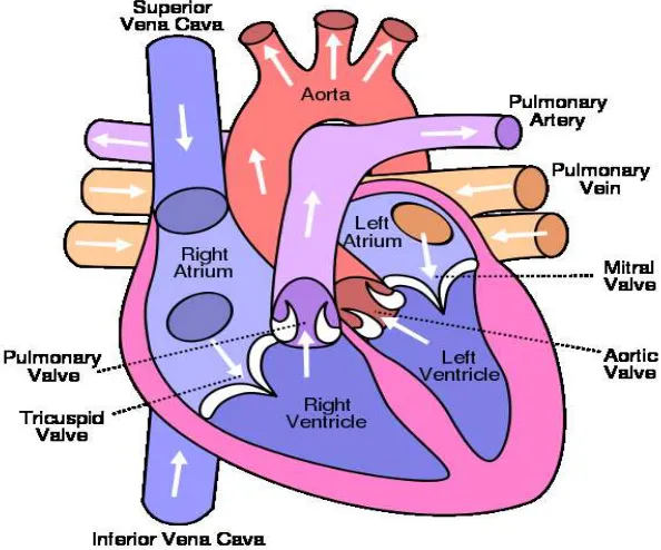
Figure 1.1: Blood Circulation. The figure is adopted from:

http://en.wikipedia.org/wiki/Circulatory_system

1.2 Blood Circulation

The heart is slightly larger than a fist, continuously pumping the blood through out the body.

The ventricles are the two main chambers of the heart that receive and send blood. The Right

Ventricle (RV) pumps the blood to the lungs and the left ventricle (LV), pumps the blood to

the whole body in each heart beat. The ventricles have thicker walls and generate higher blood

pressures comparing to the atria. Since the LV is required to pump the blood to the whole body,

its wall is thicker compared to the RV. Therefore, early and precise diagnosis of left ventricular

abnormalities plays an essential role in taking the treatment steps following prognosis.

When the heart contracts, it pushes the blood out into two major loops: a systemic loop

happens when oxygenated blood is circulated into the body and wasted carbon dioxide is

col-lected from cells; pulmonary loop happens when the blood circulates to and from the lungs in

order to release the carbon dioxide and pick up new oxygen. The systemic loop is controlled

(26)

The systemic loop begins when oxygenated blood from the lungs enters the the upper left

chamber, called the Left Atrium (LA). When the LA is filled, the mitral valve is opened by

high blood pressure and blood flows down into the LV. When the LV contracts in each heart

beat, it pushes the blood into the aorta, the largest artery of the body (usually 2 to 3cm wide).

The oxygenated blood leaving the aorta brings oxygen to the body cells through a network of

arteries and capillaries. The de-oxygenated blood from body cells returns to the heart via the

venous system. All de-oxygenated blood from the body returns to the heart by two large veins

called superior and inferior vena cavae. The superior vena cava receives blood from upper

organs of the body, while the inferior vena cava receives blood from the lower ones. Both of

these veins fill the blood into the Right Atrium (RA). The pulmonary loop begins by sending

the blood from the RA to the RV through the tricuspid valve. When the RV contracts, blood is

pushed into the pulmonary artery. The fresh, oxygen-rich blood returns to the LA of the heart

through the pulmonary veins (refer to Fig. 1.1).

Both of the circulatory system loops occur simultaneously. The contraction of the heart

muscle begins from the two atria, which forces the blood into the ventricles. Then the walls of

the ventricles contract together at the same time, pumping the blood out into the arteries. The

aorta delivers the oxygenated blood to the body, and the pulmonary artery sends the blood to

the lungs to be oxygenated. Afterwards, the heart muscle relaxes, allowing the blood to flow

in from the veins, filling the atria again for the next cycle. The heart rate is about 72 beats per

minute in a healthy individual, but can be increased or decreased in different situations. It takes

about 30 seconds for each portion of the blood to complete a full cycle (from lungs to the heart

(27)

1.3 Cardiovascular Magnetic Resonance Imaging

Magnetic Resonance Imaging (MRI) is a non-invasive imaging technique that plays an

es-sential role assessing heart conditions before and following a HF by providing accurate and

reproducible diagnostic information. It is therefore considered as the gold-standard imaging

modality for comprehensive assessments of regional and global dysfunctions of the heart [6].

Cardiac Magnetic Resonance (CMR) Images are commonly acquired at a magnetic field

strength of 1.5 T (3.0 T in some centers) [6]. This strong constant magnetic field is applied to

align the magnetization of hydrogen atoms of the organ being scanned. The hydrogen nuclei are

then excited by applying another magnetic field at a certain frequency (RF field) that deflects

their magnetization from this alignment. The signal emitted from these excited nuclei, when

they realign to their initial configuration, is measured by RF sensors and used to form an

image. In MR imaging, signals received from a particular tissue (e.g., heart muscle, fat, etc)

are determined by the density of hydrogen atoms (proton density), and by two distinct MR

relaxation parameters, longitudinal relaxation time (T1) and transverse relaxation time (T2).

Proton density, T1, and T2 are significantly varied for different tissue types, and are used to

generate contrast in MR images. Also, image contrast can be modified by modulating the way

the radiofrequency signals are applied (the MR sequence) [6].

An MR Imaging sequence refers to a specific combination of radiofrequency pulses,

mag-netic gradient field switches, and timed data acquisitions, all used to generate the MRI

im-age. In CMR, for anatomic imaging and tissue characterization, spin echo sequences are used,

whereas gradient echo sequences are used to acquire cine images which depict fat and blood

with high signal intensities. The most recent standard protocol for cardiac MR employs the

Steady-State Free Precession (SSFP) sequence. This sequence provides the best contrast

be-tween myocardium (dark) and the blood in the chamber (white) for imaging cardiac function.

For a better visualization, fat suppression sequences may be applied to allow signal from fat to

be specifically suppressed with special pre-pulses [6].

(28)

10-12 slices corresponding to a specific plane of the heart. The standard imaging plane (short

axis view) used for LV assessments is perpendicular to the long axis of the heart (apex-base).

A single cardiac MRI can therefore consist of around 200-250 short axis images, making the

analysis of such a volume of data quite challenging [6].

1.3.1 Clinical significance of using Cardiovascular Magnetic Resonance

Imaging

Cardiac MRI can image in any desired plane and with a nearly unrestricted field of view,

allowing the flexibility to evaluate abnormal structure of ventricles with different sizes and

shapes, even those that have been extensively remodeled [22,19]. The inherent 3-dimensional

nature of CMR makes it suitable for studying the RV, which is challenging to assess due to

its complex and variable morphology. Moreover, using steady-state free-precession sequences,

CMR is suitable for regional assessments of the LV because it provides excellent intensity

contrast between blood and myocardium [18]. With regard to regional ventricular function,

CMR enables accurate assessments of regional wall motion abnormalities [18].

Since CMR is accurate and reproducible [7,12,8] patients can undergo several CMR scans

without being exposed to ionizing radiation [20], making it an ideal technique for monitoring

disease treatment and progression.

It is predicted that the application of CMR imaging for patients with HF will be

substan-tially developed in the coming years [20]. Furthermore, improvements in developing CMR

software and hardware will lead to shorter scan time and, eventually, allow the use of real-time

imaging with higher spatial and temporal resolution [20].

1.3.2 Cardiovascular Magnetic Resonance Imaging Safety

In CMR scanning, the patient is not exposed to ionizing radiation, and there are no other

(29)

to the proximity of a strong magnetic field. Items with ferromagnetic materials can be pulled

into the magnet’s core with high speed, and cause serious damage that restricts application of

some equipments. However, the majority of medical implants are safe for MR scans,

includ-ing orthopedic implants, coronary and vascular stents, and prosthetic cardiac valves. Patients

with embedded ferromagnet implants such as pacemakers or defibrillators cannot be admitted

for MR scanning [20]. Currently, there are many researches on MR compatible implants and

devices that can change the development of MR machines in the future. However, when MR

compatibility of a certain device is not clear, its safety status needs to be checked by referring

(30)

1.4 Diagnosis of Cardiovascular disease

The diagnosis, treatment and follow-up of LV pathologies can rely on numerous cardiac

imag-ing modalities, which include echography, CT (Computed Tomography), coronary

angiogra-phy and MRI (cardiac Magnetic Resonance Imaging). Among others, MRI provides precise

information on morphology, tissue viability, muscle perfusion and blood flow, using suitable

protocols [13].

In clinical practice, however, assessment of the LV relies mainly on manual segmentations

as well as visual analysis and interpretations of wall motion. Several clinical studies have

shown that visual assessments are inaccurate and subject-dependent [11]. Manual

segmenta-tion of the LV is prone to intra- and inter-observer variability, therefore, automatic assessment

methods have become a major area of research [13].

Assessment of the LV includes three main steps:

1. Global assessment of the LV: This performed by estimating the cardiac Ejection

Frac-tion (EF), which is the most important observaFrac-tions in diagnosing cardiovascular diseases

because it is an important indicator of long-term prognosis for patients with coronary

artery disease. Since the LV is the main pumping chamber of the heart, the EF is usually

measured using information from the LV [20].

In current clinical practice, the EF is often estimated from several images in a cardiac

sequence using manual segmentation of the LV cavity, which is time consuming.

Auto-matic LV segmentation can also be used to compute the EF, however, the autoAuto-matic LV

segmentation techniques are challenging and computationally expensive.

2. Regional assessment of the LV: This is scored following the American Heart

Associa-tion (AHA) Standard. Heart failure is a prevalent disease that can be caused by various

heart conditions, in particular, Ischemic Heart Disease (IHD) [6]. The decrease of blood

supply produced by coronary artery stenosis impairs the contractile properties of specific

(31)

con-tractility patterns of the myocardium, especially the LV. Early and accurate detection of

LV regional wall motion abnormalities significantly helps in the diagnosis and follow-up

of IHD [1].

In routine clinical use, cardiac function is estimated by visual assessment of the LV

motion and, therefore, it is highly observer-dependent. Alternatively, computer-aided

detection systems have been attempted in recent years in order to automatically analyze

LV myocardial function quantitatively [20], and to classify cardiac function into normal

or abnormal groups [51]. The regional myocardial function is commonly scored by

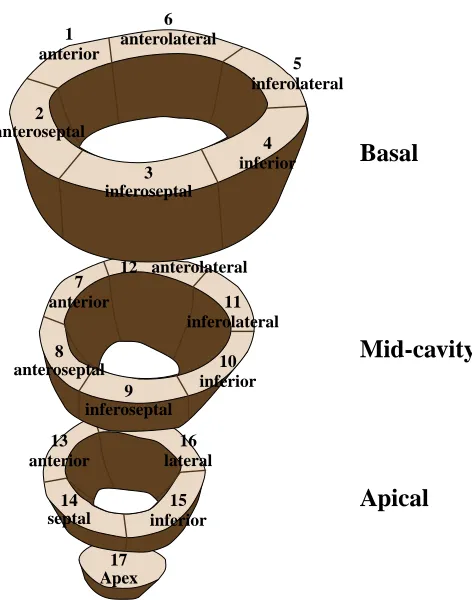
following AHA standards [2], where the LV is divided into 17 segments.

3. Classification of regional LV dysfunction: Segmental classification of the LV is widely

accepted as a predictor of cardiac disease [1]. Clinically, the regional myocardial

func-tion is also scored using AHA standards [2]. Representative 2D cardiac slices are

se-lected to generate 17 standard LV regional segments. Each of the regional segments

are assessed individually and characterized as: normal, hypokinesia, akinesia or

dyski-nesia. Distinguishing these conditions from each other is often challenging as manual

delineation of regional segments or visual assessment is used in clinical routine which is

highly subject dependent and non-reproducible [53,5]. Functional images are subject to

noise, therefore LV segmentation and regional assessment are acknowledged as difficult

problems. The difficulties come from the subtle visual differences between normal- and

abnormal-segment motions.

In this project, we propose novel methods to diagnose global and regional dysfunction of

cardiac LV using MR images, to provide a framework that will assist the radiologists in the

(32)

1.5 Global Assessment of Cardiac Left Ventricular Function

During the cardiac cycle, the heart contracts (systole) and relaxes (diastole). When the heart

contracts, it pushes the blood out of the ventricles and when it relaxes, the ventricles are refilled

with blood. Ejection Fraction (EF) is a measure of how much blood pumps out of the LV with

each heart beat.

Left ventricular Ejection Fraction (LVEF) is an important prognostic marker used to

eval-uate cardiac function globally [20]. Cardiac Magnetic Resonance (CMR) imaging provides

accurate and reproducible methods to perform physiological studies such as EF estimation. EF

is often estimated using multiple cine short -axis MR images that embrace the LV. Currently in

clinical practice, EF is estimated from several images in a cardiac sequence using manual

seg-mentation, i.e., manual delineation of the LV cavity. This is a time consuming process, which

requires about 20 to 40 min per ventricle by a clinician and is prone to intra- and inter-observer

variability. Automatic LV segmentation techniques for computing the EF has been the subject

of significant research. In particular, commercial software packages such as MASS (Medis,

Leiden, The Netherlands) [17] and Argus (Siemens Medical Systems, Germany) [46] are

to-day available for automatic ventricle delineation. Although processing time has been greatly

reduced, the provided contour detection still needs improvement compared to equal manual

contour delineation. Existing LV segmentation algorithms can be divided into the following

two main categories based on prior art [13].

1.5.1 Left Ventricle segmentation based on no or weak priors:

In general, LV segmentation approaches with no or weak priors are image-driven. Existing

algorithms are based on thresholding [18, 29, 62, 45, 28, 35], dynamic programming [15,

64,17], shortest path algorithms [23], pixel classification via Gaussian Mixture Models [48]

or clustering [10], and deformable models which evolve and regularize a curve following

(33)

approaches do not require intensive training. However, in order to compensate the lack of

spatial information, they generally resort to user interventions or several pre- or post-processing

steps to localize the LV. This section summarizes segmentation methods with weak or no prior,

including image-based, pixel classification-based and deformable models.

Image-Based Methods

The majority of the image-based methods involve a two-steps process to individually segment

the endo and epicardium [13]. The first step focuses on detecting the endocardial boundary

us-ing thresholdus-ing [18,29,62,45,28,35] or dynamic programming [17,19,32]. The epicardial

boundary is delineated during the second step, often based on the endocardium boundary using

a spatial model. The model utilizes information about myocardial thickness or mathematical

morphology operators.

Pixel Classification

Pixel classification methods are often used when multiple images of the same organ are

avail-able, e.g., multiple MRI or multi-modality images. The image is divided into different regions

or classes that have similar feature values. Segmentation can be performed using either

su-pervised (with learning datasets) or unsusu-pervised techniques (without training datasets). In

[48], Pednekar et al. used Gaussian Mixture Model (GMM), to fit the image histogram, and

clustering.

Deformable Models

Segmentation methods based on deformable models use active contours or snakes [27], and

are based on deforming a curve iteratively to minimize an energy function. The energy

func-tion consists of two main components; a regularizafunc-tion term controlling the smoothness of the

curve and a data term that includes information about object boundary. The curve evolution

(34)

im-plementation of curve evolution, the level-set framework is widely used in medical imaging

because of its flexibility regarding topological changes. The level-set method facilitates

seg-mentation of multiple objects. Deformable models have been used widely for LV segseg-mentation

[24,63,41,3].

Almost all of the methods using weak priors or none at all require user intervention. In

order to fully automate the process, incorporating strong spatial priors (e.g. relating to the the

shape of the target region) has been researched for LV segmentation. Section 1.5.2. discusses

some of the existing methods within this direction.

1.5.2 Left Ventricle segmentation based on strong priors

Automatic LV segmentation is generally based on strong spatial priors such as statistical shape

models or atlases. This is especially true if the shape of the target region does not change

significantly from one subject to another, which is a reasonable assumption for the LV. Such

strong priors can relax the need for user intervention, but at the expense of manually building a

large training set. Methods falling within this category are based on shape-driven deformable

models [47,36,39, 40], Active Shape Models (ASM) [66,65], and atlas based models [37,

68].

Shape-driven Deformable Models

Shape-driven deformable models evolve an active curve/surface according to the minimization

of an energy functional, comprising a set of template shapes learned a priori. The evolution

equation is computed by minimization of the functional, which contains a statistical shape

constraint. The principle is to modify the energy functional by adding a new term that embeds

a shape constraint, such as a distance to a reference shape model, e.g., the mean signed distance

map as used by Paragios et al. to build a reference shape [47, 36]. A Probability Density

Function (PDF) or probabilistic map can be estimated by using manual LV segmentations, and

(35)

Active Shape Models

The Active Shape Model (ASM) consists of two steps: (1) building a statistical shape model

following a Principal Component Analysis (PCA) of a set of aligned training shapes, and (2)

finding a segmentation in the current image by fitting the solution to the learned model and

estimating rotation, translation and scaling parameters [66,65,4]. Active Appearance Models

(AAM) are an extension of ASM by modeling gray levels [13] that include both shape and

texture variability in the training set.

Atlas Based models

In atlas based methods, an image is segmented by mapping its coordinate space to that of an

at-las, often following a registration process. This technique has been used for heart segmentation

[37, 67, 11]; the principle is to register the labeled atlas onto the image to be segmented, and

then apply the obtained transformation to the atlas, thereby obtaining the final result. The result

can then be propagated over time throughout the cardiac cycle following the same principle.

1.5.3 The Proposed Method

In this project, we propose estimating the EF without segmentation in real-time directly from

image statistics using machine learning techniques. From a simple user input in only one

image, we build a statistic based on the Bhattacharyya coefficient [14] of similarity between

image distributions for all the images in a subject dataset . We demonstrate that these statistics

are non-linearly related to the LV cavity areas and, therefore, can be used to estimate the EF

via an Artificial Neural Network (ANN) directly. The proposed method consists of four main

steps:

1. Image acquisition

(36)

3. Applying Artificial Neural Networks

(37)

1.6 Regional Assessment of Cardiac Left Ventricular

Func-tion

Accurate detection of segmental (regional) LV abnormalities in MRI is accepted as a predictor

of cardiac diseases, the leading cause of death worldwide [6]. In clinical practice,

segmen-tal cardiac function (Fig. 1.2) is considered an essential diagnosis and follow-up component

[1]. It is often assessed visually following the AHA standard [2], which prescribes selecting

representative 2D cardiac slices used to generate 17 standardized LV segments. Currently

radi-ologists visually assess the 17 segments together. These practices, along with being subject to

high inter-observer variability [5,53], and are subjective and non-reproducible. For instance,

the clinical study in [5] showed that the mean kappa measure of detecting regional wall

mo-tion abnormalities by three different radiologists could be as low as 0.43, the difficulties coming

from the subtle visual differences between normal- and abnormal-segment motions. Automatic

diagnosis of LV regional dysfunction has attracted significant research [15,11,21,4, 14, 10].

Regardless of promising performances of the applied techniques, the results can still be

im-proved in terms of accuracy. For instance, the recent publication in [21] reports an accuracy of

63.70% (base), 67.41% (middle), and 66.67% (apex) when visual wall motion scoring is used

as reference.

1.6.1 Prior art

Echocardiography Based Methods

Most of the pioneering studies of wall motion abnormality detection targeted echocardiography

[3,9,12], using concepts from shape statistics [3,9] and Hidden Markov Models (HMM) [12],

among others. In [3], model-based shape analysis is used to automatically classify wall motion

abnormalities in echocardiograms. The shape model is obtained using Principle Component

(38)

17 Apex 13 16 15 14 anterior septal inferior lateral 7 12 11 10 9 8 anterior anteroseptal inferoseptal inferior inferolateral anterolateral 1 2 3 4 5 6 anterior anteroseptal inferoseptal inferior inferolateral anterolateral Apical Mid-cavity Basal

Figure 1.2: AHA standard for LV regional segments.

In this particular example, they used PCA to find the average endocardial shape and large

eigenvectors representing the main modes of variations. Any shape in the testing dataset can

be represented by a combination of average shapes and a specific linear combination of these

eigenvectors. The eigenvectors correspond to regional wall motion abnormality. Multivariate

linear regression was then applied to differentiate normality and abnormality of the regional

segments.

In [9], the authors built sparse shape models with localized variations from four- and

two-chamber echocardiographic sequences using principal component analysis and orthomax

rotations. Then, the ensuing shape parameters were used to assess local wall motion.

In [12], Mansor et.al. investigated a HMM as a tool for regional stress cardiography wall

motion abnormality detection. HMM are especially known for their application in temporal

pattern recognition [22] because of their ability to successfully learn the time-varying

(39)

sequential properties. First, the myocardial contour was semi-automatically delineated using

Quamus software. Next, each contour was divided into six parts, and several features were

extracted to evaluate the wall motion. The data was then separated into two groups of normal

and abnormal subjects. Two HMMs were then developed for each segment. Finally, the trained

HMM was used to evaluate regional wall motion for the new dataset.

Magnetic Resonance Imaging Based Methods

More recently, MRI-based wall motion abnormality detection has been studied [15, 11, 21, 4,

14,10]. In [14], Punithakumar et al. characterized myocardial-segment motions via a

nonlin-ear dynamic model, and used the Shannon’s differential entropies of various segment features

(e.g., areas and radial distances) as inputs of a naive Bayes classifier. They investigated the

problem with a global measure based on the Shannon’s Differential Entropy (SDE) of

distri-butions of normalized radial distances, radial velocities and segment areas. As discussed in

[14], SDE measures global distribution information, and is more discriminative in

classify-ing distributions compared to the methods that rely on elementary measures or a fixed set of

moments.

In [21, 19], Suinesiaputra et al. built normokinetic myocardial shape models using

short-axis MR images acquired from healthy volunteers. They proposed using an Independent

Com-ponent Analysis (ICA) classifier that detects and localizes abnormally contracting segments,

via a characterization of local shape variations.

Lekadir et al. [10] focused on statistical modeling based on spatio-temporal inter-landmark

relationships.

In [11], Lu et al. proposed a pattern recognition technique built upon intra-segment

corre-lation, using a normalization scheme which maps each LV slice to polar coordinates with fixed

size, intensity level, and position.

The study in [4] proposed a differentiable-manifold analysis, following differential

(40)

manifold.

The authors of [15] investigated a tensor-based Linear Discriminant Analysis (LDA)

clas-sification that conserves the spatio-temporal structure of the myocardial function. Radial and

circumferential strain as well as tissue-rotation angle were used as features to train and test a

classifier via manual segmentations of the myocardium.

Most of the existing methods require delineations of the endo- and/or epi-cardial

bound-aries in all frames of a cardiac sequence, using either a manual time-consuming process [4,

21, 11, 15] or an automatic/semi-automatic segmentation (delineation) algorithm [14]. As

discussed in section 1.5. segmentation algorithms are either sensitive to user inputs and/or are

computationally expensive and may result in high estimation errors [13]. Furthermore, the

segmentation results often depends on the choice of parameters and training dataset. These

difficulties inherent to segmentation algorithms prevent their clinical adoption for segmental

motion abnormality detection. Moreover, some of the existing algorithms, e.g., those based on

shape analysis techniques [21], require such delineations in the training phase, which increases

the amount of manual input and training complexity.

1.6.2 The Proposed Method

In this thesis, we propose a regional myocardial abnormality detection framework based on

image statistics. The proposed framework requires minimal user interaction, with the clinician

only needing to specify initial delineation and anatomical landmarks on the first frame.

Ap-proximations of regional myocardial segments in subsequent frames were systematically

ob-tained by superimposing the initial delineation on the rest of the frames. The proposed method

exploits the Bhattacharyya coefficient to measure the similarity between the image distribution

within each segment approximation and the distribution of the corresponding user-provided

segment. Linear Discriminant Analysis (LDA) is applied to find the optimal direction along

which the projected features are the most descriptive. Then a Linear Support Vector Machine

(41)

detect abnormally contracting regions of the myocardium. Based on a clinical dataset of 58

subjects, the evaluation demonstrates that the proposed method can be used as a promising

diagnostic support tool to assist clinicians. The proposed method consists of four main steps:

2. Building Image Statistics

3. Applying Linear Discriminant Analysis

(42)

1.7 Multi-Class Segmental Cardiac Dysfunction

Classifica-tion of Cardiac Left Ventricular FuncClassifica-tion

In routine clinical procedures, segmental cardiac function is considered an essential

diagno-sis and follow-up component [1]. It is commonly scored following the AHA standard [2]

which prescribes dividing the LV into 16 regional segments, each assessed individually and

characterized as:

• normal

• hypokinesia: reduced LV contraction

• akinesia: absence of contraction

• dyskinesia : bulging out in systole

Current radiologic practices rely on visual assessment, which is subject to a high

inter-observer variability, while being subjective and non-reproducible [53, 5]. Furthermore, visual

assessment requires either manual delineation of the segments in all the frames of a subject

dataset, which is prohibitively time-consuming, or automatic delineation, which is a

challeng-ing computational problem [13].

1.7.1 Prior Art

Automating LV abnormality scoring has been the subject of numerous recent studies as

dis-cussed in section 1.6 [19, 4, 14, 2, 21, 15, 12]. Earlier studies of wall motion abnormality

detection used various approaches including differentiable manifolds [4], independent

compo-nent analysis classification [21], information-theoretic techniques [14], tensor-based

classifi-cation [12], and image statistics based classification [2].

Unfortunately, to the best of our knowledge, all existing algorithms address a binary

(43)

Fur-thermore, most of the existing methods require LV segmentation in all frames of a cardiac

sequence. As noted earlier, this is either done manually which is time consuming or

automati-cally with its associated drawbacks [4,21,15]).

1.7.2 The Proposed Method

We propose a method to solve this problem using image statistics from MR images. The

pro-posed method requires minimal user-interaction with the clinicians only needing to delineate

the inner and outer boundary and two anatomical landmarks of the LV in one single frame of

cine MRI sequence. The obtained outer boundary is then systematically superimposed to all

other corresponding frames with no changes. The amount of blood inside the regional LV

cav-ity is modeled by Bhattacharyya statistics between distribution estimated inside the LV cavcav-ity

of first frame and regional segments in the rest of the frames. The muscle inside the regional LV

is modeled using the same idea from Bhattacharyya statistics between distributions estimated

inside the LV myocardium of the first frame and regional segments in the rest of the frames.

A Support Vector Machine (SVM), is then used to find the correlation between the estimated

image statistics and different regional abnormalities of the LV. The results show that the image

statistics can be used to differentiate among various LV abnormalities. The algorithm shows

comprehensive results on 174_∗20 short axis segments, obtained from 58 subjects. The method

diagnoses the condition of LV regional segments with 74.14% accuracy. The proposed method

consists of four main steps:

2. Building Image Statistics

3. Applying Support Vector Machine

(44)

1.8 Thesis Objectives

The main objective of this work is to provide a platform to assist radiologists in diagnosis

of LV abnormalities. We developed a new automated tool to mimic the different steps of

the diagnostic procedures, to automatically assess cardiac function. This platform has the

potential to be further developed into a product for diagnosis of cardiac dysfunction, providing

radiologists with an accurate and fast system that can be integrated with MRI scanners.

Specific research objectives are listed below:

• Develop a software system for the diagnosis of LV dysfunction that would be compatible

with MRI scanners.

• Provide clinicians with a fast and accurate diagnostic tool that assesses the LV function

globally with a minimal user input.

• Presenting MRI features that could be used to directly assess cardiac functions in terms

of global dysfunction without the need for segmentation.

• Develop a tool to estimate the regional cardiac function automatically with a minimum

user-intervention.

• Speed up the procedure of automatically assessing segmental LV by removing the need

for segmentation while exceeding the accuracy of current systems.

(45)

1.9 Thesis Outline

1.9.1 Chapter 2: Global Assessment of Cardiac Left Ventricle Function

Using Estimation of Ejection Fraction

This chapter describes how we design a diagnostic tool for global assessment of cardiac

func-tion using estimafunc-tion of EF. In clinical routine, EF is often estimated by either manual or

auto-matic segmentation of the LV in number of short axis CMR Images. In general, the

segmen-tation algorithms discussed in section 1.5 require careful user interventions and/or intensive

manual training, along with a heavy computational load. Furthermore, the ensuing

segmenta-tion results depend significantly on the choice of a set of parameters and training data, causing

high errors in the EF estimation. These difficulties inherent to segmentation algorithms limit

the automatic estimation of the EF in routine clinical use.

While existing techniques are labour intensive, we believe that there are other

character-istics of the images that can be computed with less effort, but that nevertheless correlate with

the EF. One such technique that we describe in chapter two is based on machine learning

tech-nique, which removes the need for image segmentation. We build an image statistic for every

image in a subject dataset using a simple user input in a single image. We show that there

is a non-linear relation between these statistics and the LV cavity areas (cf. Figs. 2.7 -2.12).

Therefore the EF can directly be estimated using the statistics in real-time via an Artificial

Neural Network (ANN). We Perform a comprehensive evaluation on 20 subject datasets and

demonstrate that the estimated EFs are very well correlated with those obtained from manual

(46)

1.9.2 Chapter 3: Regional Assessment of Cardiac Left Ventricle

Func-tion

Regional assessment of cardiac LV function is based on the segmentation of the LV in either

the entire cardiac cycle or several frames. Indeed, there are other image characteristics that can

be estimated with minimum user interaction. These characteristics correlate with segmental

cardiac dysfunction. One such technique that we describe in chapter three is based on image

features and machine learning, which removes the need for delineating the endo- and

epi-cardial boundaries in all the images of a cardiac sequence. Starting from a minimum user input

in only one frame in a subject dataset, we build, for all the regional segments and all subsequent

frames, a set of statistical MRI features based on a measure of similarity between distributions.

We demonstrate that, over a cardiac cycle, the statistical features are related to the proportion

of blood within each segment. Therefore, they can characterize segmental contraction without

the need for delineating the LV boundaries in all the frames. We first find the optimal direction

along which the proposed image features are most descriptive via Linear Discriminate Analysis

(LDA). Then, using these results as inputs to a Linear Support Vector Machine (LSVM)

clas-sifier, we obtain an abnormality assessment (normal/abnormal) of each of the standard cardiac

segments in real-time. We report a comprehensive experimental evaluation of the proposed

algorithm over 928 cardiac segments obtained from 58 subjects. Compared against

ground-truth evaluations by experienced radiologists, the proposed algorithm yielded a competitive

performance, with an overall classification accuracy of 86.08% and a kappa measure of 0.73.

1.9.3 Chapter 4: Multi-Class Segmental Cardiac Dysfunction

Classifica-tion

The purpose of this chapter is to investigate the more general and challenging multi-class

prob-lem, where each regional segment is classified into one of four classes: (1) normal; (2)

(47)

the given subject. Using this input we build for all the regional segments and all subsequent

frames a set of statistical MRI features based on a measure of similarity between distributions.

Over a cardiac cycle, these statistical features are related to the proportion of blood and

my-ocardium within each segment, and can therefore characterize segmental cavity/myocardium

contraction without the need for delineating the LV boundaries in all the frames. Finally, using

these features as inputs to a multi-class Support Vector Machine (SVM) classifier, we obtain

a 4-class assessment of each segment. We report a comprehensive experimental evaluation of

the proposed algorithm over 928 cardiac segments obtained from 58 subjects. Compared to

ground-truth labels assessed by an experienced radiologist, the proposed algorithm yielded an

overall 4-class accuracy of 74.14%.

1.9.4 Chapter 5: Summary, Contribution and Future Directions

This chapter summarizes the contribution of this project, and discusses the limitations were

faced at different stages. Suggestions and future directions are included to extend this project

(48)

References

[1] H. Abdel-Aty, O. Simonetti, and M. G. Friedrich, “T2-weighted cardiovascular magnetic

resonance imaging,” Journal of Magnetic Resonance Imaging, vol. 26, no. 3, pp. 452–459,

2007.

[2] M. Afshin, I. Ben.Ayed, K. Punithakumar, M. W. K. Law, A. Islam, A. Goela, I. G. Ross,

T. M. Peters, and S. Li, “Assessment of regional myocardial function via statistical

fea-tures in MR images,” in Medical Image Computing and Computer-Assisted Intervention;

MICCAI, 2011, pp. 107–114.

[3] B. R. Annuar, C. K. Liew, S. P. Chin, T. K. Ong, M. T. Seyfarth, W. L. Chan, Y. Y. Fong,

C. K. Ang, N. Lin, H. B. Liew, and K. H. Sim, “Assessment of global and regional left

ventricular function using 64-slice multislice computed tomography and 2d

echocardiog-raphy: A comparison with cardiac magnetic resonance,” European Journal of Radiology,

vol. 65, no. 1, pp. 112 – 119, 2008.

[4] I. Ben Ayed, K. Punithakumar, A. Islam, J. Chong, and S. Li, “Left ventricle segmentation

via graph cut distribution matching,” in Medical Image Computing and Computer-Assisted

Intervention; MICCAI, vol. 5762, 2009, pp. 901–909.

[5] I. Ben Ayed, I. Ross, and S. Li, “Embedding overlap priors in variational left ventricle

tracking,” IEEE Transaction on Medical Imaging, vol. 28, no. 12, pp. 1902–1913, 2009.

[6] G. S. Bleumink, A. M. Knetsch, M. C. Sturkenboom, S. M. Straus, A. Hofman, J. W.

(49)

Preva-lence, incidence rate, lifetime risk and prognosis of heart failure - the rotterdam study,”

European Heart Journal, vol. 25, pp. 1614–1619, 2004.

[7] J. G. Bosch, F. Nijland, S. C. Mitchell, B. P. Lelieveldt, O. Kamp, J. H. Reiber, and

M. Sonka, “Computer-aided diagnosis via model-based shape analysis: Automated

classi-fication of wall motion abnormalities in echocardiograms,” Academic Radiology, vol. 12,

no. 3, pp. 358 – 367, 2005.

[8] G. Buckberg, “Left ventricular form and function: Scientific priorities and strategic

plan-ning for development of new views of disease,” Circulation, vol. 110, pp. e333–e336,

2004.

[9] M. D. Cerqueira, N. J. Weissman, V. Dilsizian, A. K. Jacobs, S. Kaul, W. K. Laskey, D. J.

Pennell, J. A. Rumberger, T. Ryan, and M. S. Verani, “Standardized myocardial

segmen-tation and nomenclature for tomographic imaging of the heart,” Journal of the American

Heart Association, vol. 105, pp. 539–542, 2002.

[10] C. A. Cocosco, W. J. Niessen, T. Netsch, E. P. A. Vonken, G. Lund, A. Stork, and M. A.

Viergever, “Automatic image-driven segmentation of the ventricles in cardiac cine MRI,”

Journal of Magnetic Resonance Imaging: JMRI, vol. 28, no. 2, pp. 366–374, 2008.

[11] L. D. Collins, A. P. Zijdenbos, W. F. C. Baare, and A. C. Evans, “ANIMAL+INSECT:

Improved Cortical Structure Segmentation,” International Conference on Information

Pro-cessing in Medical Imaging (IPMI), vol. 1, pp. 210–223, 1999.

[12] D. Comaniciu, V. Ramesh, and P. Meer, “Kernel-based object tracking,” IEEE

Transac-tions on Pattern Analysis and Machine Intelligence, vol. 25, no. 5, pp. 564–577, 2003.

[13] T. Cootes, G. Edwards, and C. Taylor, “Active appearance models,” Proceedings of the

(50)

[14] T. F. Cootes, C. J. Taylor, D. H. Cooper, and J. Graham, “Active shape models, their

training and application,” Computer Vision and Image Understanding, vol. 61, no. 1, pp.

38–59, 1995.

[15] J. Cousty, L. Najman, M. Couprie, S. C. Guinaudeau, T. Goissen, and J. Garot,

“Segmen-tation of 4D cardiac MRI: automated method based on spatio-temporal watershed cuts,”

Image and Vision Computing, vol. 28, no. 8, pp. 1229–1243, 2010.

[16] J. Garcia-Barnes, D. Gil, L. Badiella, A. Hern`andez-Sabat´e, F. Carreras, S. Pujadas, and

E. Mart´ı, “A normalized framework for the design of feature spaces assessing the left

ventricular function,” IEEE Transaction on Medical Imaging, vol. 29, no. 3, pp. 733–745,

2010.

[17] R. van der Geest, E. Jansen, V. Buller, and J. Reiber, “Automated detection of left

ven-tricular epi- and endocardial contours in short-axis MR images,” Computers in Cardiology,

vol. 1, pp. 33–36, 1994.

[18] A. Goshtasby and D. Turner, “Segmentation of cardiac cine MR images for extraction

of right and left ventricular chambers,” IEEE Transactions on Medical Imaging, vol. 14,

no. 1, pp. 56 – 64, 1995.

[19] A. Gupta, L. von Kurowski, A. Singh, D. Geiger, C.-C. Liang, M.-Y. Chiu, L. Adler,

M. Haacke, and D. Wilson, “Cardiac MR image segmentation using deformable models,”

IEEE Conference on Computers in Cardiology, vol. 1, pp. 747–750, 1993.

[20] H. C. Han, R. P. Martin, G. Lerakis, and S. Lerakis, “Prediction of the left ventricular

ejection fraction improvement using echocardiography and mechanical modeling,” Journal

of the American Society of Echocardiography, vol. 18, no. 7, pp. 718–721, 2005.

[21] R. Hoffmann, S. von Bardeleben, J. D. Kasprzak, A. C. Borges, F. ten Cate, C. Firschke,

Automatic Assessment of Cardiac Left Ventricular Function Via Magnetic Resonance Images

Scholarship@Western

Scholarship@Western

Automatic Assessment of Cardiac Left Ventricular Function Via

Automatic Assessment of Cardiac Left Ventricular Function Via

Magnetic Resonance Images

Magnetic Resonance Images

AUTOMATIC ASSESSMENT OF CARDIAC LEFT VENTRICULAR

FUNCTION VIA MAGNETIC RESONANCE IMAGES

(Thesis format: Integrated Article)

by

Mariam Afshin

Graduate Program in Biomedical Engineering

Submitted in partial fulfillment

of the requirements for the degree of

Doctorate of Philosophy

The School of Graduate and Postdoctoral Studies

Western University

London, Ontario, Canada

c

WESTERN UNIVERSITY

School of Graduate and Postdoctoral Studies

CERTIFICATE OF EXAMINATION

Abstract

Acknowlegements

Contents

List of Figures

List of Tables

List of Abbreviations

List of Appendices

Chapter 1

Introduction

1.1

Heart Failure

1.2

Blood Circulation

1.3

Cardiovascular Magnetic Resonance Imaging

1.3.1

Clinical significance of using Cardiovascular Magnetic Resonance

Imaging

1.3.2

Cardiovascular Magnetic Resonance Imaging Safety

1.4

Diagnosis of Cardiovascular disease

1.5

Global Assessment of Cardiac Left Ventricular Function

1.5.1

Left Ventricle segmentation based on no or weak priors:

1.5.2

Left Ventricle segmentation based on strong priors

1.5.3

The Proposed Method

1.6

Regional Assessment of Cardiac Left Ventricular

Func-tion

1.6.1

Prior art

1.6.2

The Proposed Method

1.7

Multi-Class Segmental Cardiac Dysfunction

Classifica-tion of Cardiac Left Ventricular FuncClassifica-tion

1.7.1

Prior Art

1.7.2

The Proposed Method

1.8

Thesis Objectives

1.9

Thesis Outline

1.9.1

Chapter 2: Global Assessment of Cardiac Left Ventricle Function

Using Estimation of Ejection Fraction

1.9.2

Chapter 3: Regional Assessment of Cardiac Left Ventricle

Func-tion

1.9.3

Chapter 4: Multi-Class Segmental Cardiac Dysfunction

Classifica-tion