Electromagnetic Tethers as Deorbit Devices - Numerical Simulation of an Upper-Stage Deorbit Efficiency

(1)

Copyright to IJAREEIE DOI:10.15662/IJAREEIE.2015.0410089 8348

Electromagnetic Tethers as Deorbit Devices -

Numerical Simulation of an Upper-Stage

Deorbit Efficiency

Alexandru Ionel

INCAS - National Institute for Aerospace Research, Romania

ABSTRACT:

This paper examines the deorbit efficiency of an electromagnetic tether deorbit device when used to deorbit an upper stage at end of mission from low Earth orbit. This is done via a numerical simulation in Matlab R2013a, using ode45, taking into account perturbations the upper stage’s trajectory. The perturbations considered atmospheric drag, 3rd body (Sun and Moon), and Earth’s gravitational potential expanded into spherical harmonics.

KEYWORDS:

Electromagnetic Tether, Orbital Debris, Deorbit Devices, ode45, Spherical Harmonics, 3rd body Perturbation

I.ORBITAL DEBRIS ISSUES

(2)

II. ELECTROMAGNETIC TETHERS AS DEORBIT DEVICES

As pointed out in [6], the use of tether technology in space missions can be grouped in eight categories of applications, categories which specify the scientific field which utilizes tether technologies in space missions. These categories are the following: aerodynamics (i.e. station tethered express payload systems, multiprobe for atmospheric studies), concepts (i.e. gravity wave detections using tethers, Earth-Moon tether transport systems), controlled gravity (i.e. rotating controlled gravity laboratory, tethered space elevator), electrodynamics (i.e. electrodynamic power generation, electrodynamic thrust generation), planetary (i.e. Jupiter inner magnetosphere maneuvering vehicle, Mars tethered observer), science (i.e. science applications tethered platform, tethered satellite for cosmic dust collection), space station (i.e. microgravity laboratory, attitude stabilization and control), transportation (i.e. tether reboosting of decaying satellites, tether rendezvous system).

Electrodynamic applications of tethers include electrodynamic power generation, electrodynamic thrust generation and ULF/ELF/VLF communications antenna. The possible use of the electrodynamic power generation or electrodynamic brake or drag concept is the generation of DC electrical power to supply primary power to on-board loads. A description of the applied concept is the following: a spacecraft is connected to a subsatellite through an insulated conducting tether, with plasma contactors used at both tether ends, and the motion through the geomagnetic field induces a voltage across the tether, so that DC electrical power is generated at the expense of spacecraft or tether orbital energy. The space missions which proved the electrodynamic brake or drag concept were TSS-1 (1992), TSS-1R (1996) and the PMG (Plasma Motor Generator) flights (1993).

The electrodynamic power generation concept and practice showed that a tethered space system of mass 900 to 19000 kg, having an aluminum tether of length 10 to 20 km produces approximately 1kW to 1MW power.

The generation of electrodynamic thrust can be used to boost the orbit of a spacecraft. Concept description: current from a spacecraft’s on-board power supply is fed into the conducting, insulated tether (which connects the spacecraft and a possible subsatellite) against the electromagnetic force induced by the geomagnetic field, producing a propulsive force on the spacecraft or tether system. The TSS-1, TSS-1R and PMG missions have demonstrated this principle. The application of the generation of electrodynamic thrust concept implies that a tethered system of mass between 100 and 20000 kg, having am aluminum tether of length between 10 and 20 km produces thrust of up to 200 N, being powered with up to 1.6 MW.

The electrodynamic drag concept is based on the exploitation of the Lorentz force due to the interaction between the electric current flowing in a conducting tether and the geomagnetic field. The motion of the conducting tether through the Earth’s magnetic field will generate a voltage along the tether. The electromagnetic interaction of a conducting tether deployed from an upper stage launcher vehicle at EOM (end of mission), moving at orbital speeds across Earth’s magnetic field will induce current flow along the tether, provided there exists a means for the tether to make electrical contact with the ambient plasma, such as a hollow cathode plasma contactor, field emission device or a bare wire anode. The electron current is leaving the space plasma and entering the tether near the end so the current will flow upwards through the tether, towards the upper stage body.

(3)

III. DESCRIPTION OF THE WORK LOGIC

The system to be simulated numerically will be composed of the following elements: a fixed inertial frame, represented by the Earth, around which all the other elements are revolving, meaning the upper-stage in an elliptical orbit around the Earth, the Moon in an elliptical orbit around the Earth, and for simplicity, the Sun in an elliptical orbitaround the Earth. The Moon and Sun’s orbital positions in time were projected with the Lagrange coefficients. The time variant orbital position of the upper stage in orbit around the Earth was calculated by integrating with respect to time the Earth’s gravitational potential and the following orbital perturbations: the Moon’s gravitational influence, the Sun’s gravitational influence, solar radiation pressure and atmospheric drag. In the solar radiation pressure calculations the upper stage’s position in the Earth’s and Moon’s cylindrical shadow was considered and also the indirect solar radiation pressure coming from the sunlight reflected from Earth’s surface. The state vectors of the upper stage, the Moon and the Sun are shown in (1), (4) and (5), while (2) shows the time derivative of the upper-stage’s state vector. Earth’s gravitational potential was expanded in 2nd order spherical harmonics dependent on latitude. The integration of (2) over time, to find out the upper-stage’s orbital position was done in Matlabusing the ode45 solver. (3) describes the general formula for the velocity derivation, in which 𝒂𝑝 represents all the perturbations acting on the upper-stage, including

Earth’s ellipticity. In the following sections the equations used to describe the perturbations and objects’ orbital positions will be shown, ending with the numerical simulation environment presentation and the simulation results. Lastly, conclusions and future work statements will be presented.

IV. GEOPOTENTIAL EQUATIONS

Generally, the gravitational potential can be expressed with the use of (6), in which 𝐺 = 6.67384 ∙ 10−11_𝑚3_𝑘𝑔−1_𝑠−2_,

and is gravitational constant, 𝑀 = 5.972 ∙ 1024_𝑘𝑔_{, and is the mass of the Earth and}_𝑟_{is the distance from the point of}

interest, 𝑃, to the centre of the Earth, as shown in Figure 1.

GM

U

r

 

(6)

G

dU

dM

q

 

(7)

(6) holds true for a point mass 𝑀. For this study we will consider the Earth a prolate spheroid. (7) will be used, where

𝑞 = (𝑟2_{+ 𝑠}2_{− 2𝑟𝑠 cos 𝜑)}1/2_and1

(4)

Figure 1: The potential U of the aspherical body is calculated at point P, which is external to the mass

M





dM

; OP= r, the distance from the observation point to the center of mass. Note that r is constant and the s, q and θ are the variables. There is no rotation so U(P) represents the gravitational potential

The gravitational potential on a point P is now given by (8).

2 2 2 2 2

2 3 3 3 3

3

3 ( )

cos

sin

2

2 G

G

U P

dM

s

dM

s dM

s

dM

r



r





_



_



_



_



_



_

(8)

The second term of (8) vanishes, the third term represents the moment of inertia and can be written as (9) or more generally as (10). The fourth term of (8) represent the moment of inertia around OP and will be noted as 𝐼.

2 2 2 2 2 2 2

3 3

(

)

(

)

(

)

2 G

G

s dM

y

z dM

x

z dM

x

y

dM

r







_



_



(9)





2

3 3

G

s dM

A B C

r





r

 

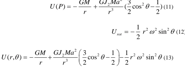
(10)

For a spheroid we can take 𝐴 = 𝐵 ≠ 𝐶, 𝐼 = 𝐴 + (𝐶 − 𝐴) cos2_𝜃_and_{𝐶 − 𝐴 = 𝐽}

2𝑀𝑎2 so (8) becomes (11). 𝐽2=

0.0010826. The rotational potential of the Earth is denoted by (12). So the Geopotential can be written as (13), in which 𝑎 = 6378.1𝑘𝑚 is Earth’s radius at the equator and 𝜔 = 7.367 ∙ 10−5_{𝑟𝑎𝑑/𝑠}_{is the angular velocity of rotation of}

the Earth. 2 2 2 3

3

1 ( )

( cos

)

2

2 GJ Ma

GM

U P

r



 





(11)

2 2 2

1 sin

2

rot

U

 

r





(12)

2

2 2 2 2

2 3

3

1

1 ( , )

cos

sin

2

2 GJ Ma

GM

U r

r



 





_







_











(13)

(5)

2

2 2 2 2

2 3

3

1

1 ( , )

sin

cos

2

2 GJ Ma

GM

U r

r



 





_







_











(14)

Now, considering 𝑐 the polar radius, 𝑓 =𝑎−𝑐

𝑎 the geometric flattening of the Earth, 𝑟𝜆 = 𝑎(1 − 𝑓 sin

2_𝜆)_{the Earth’s}

radius at latitude 𝜆, (15) shows the final expression of the Earth’s Geopotential in terms of latitude 𝜆.

The Geopotential at altitude 𝑕 above Earth’s surface was calculated using equation (16), in which 𝑟𝑢𝑠 represents the

magnitude of the upper-stage’s position vector with respect tothe ECEF frame.

2

2 2 2 2

2

2 2 2 4 2 4

3

1 ( )

sin

(1

sin

) cos

2

2 (1

sin

)

(1

sin

)

E

GM

GJ Ma

g

a

f

a

f

a

f











 



_



_







(15)

2 2

(1

sin

)

( , )

( )

us

a

f

g

h

g

r









_





_





(16)

V. LUNAR ORBIT AND THIRD BODY PERTURBATION

The Moon’s state vector at each instant in time will be calculated using (17) and (18), having been supplied the initial values 𝒓𝑀0and 𝒗𝑀0. 𝑓and𝑔 in (19) and (20) represent the Lagrange coefficients, with 𝑓 and 𝑔 being their time

derivatives. 𝐶(𝑧)and𝑆(𝑧) are Stumpff functions. 𝜒represents the universal anomaly, which at 𝑡0= 0 is 𝜒𝑡₀= 0.𝜇𝑀is

(6)

sin , 0

( ) sin , 0

1 , 0 6

z z z

S z z z z

z             

 ₍₂₄₎

1 cos

, 0

cosh 1

( ) , 0

1 , 0 2 z z z z

C z z

z z   _        _    _ 

 ₍₂₅₎

2 3 0 0 0 1 2 0 0 0

1 ( ) (1

)

( )

1

1 ( )

ro

i i i i i

M

i i

ro

i i i i

M M

r v

C z

r

S z

r

t

a

r v

S z

r

C z

r

a









 

 







 





 

_

_









 





(26)

After we have found the Moon’s position at each moment in time, we need to find out the orbital elements at each instant so as to use them in the upcoming third body perturbation formula. The following algorithm,defines the orbital elements, where 𝑟 is the Earth – Moon distance, 𝑣 is the Moon’s orbital speed, 𝑣𝑟 is the Moon’s radial speed, 𝑕 is the

(7)

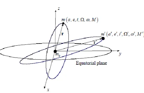
Copyright to IJAREEIE DOI:10.15662/IJAREEIE.2015.0410089 8354 Having found the orbital elements at each moment in time we will use, we shall continue to describe the Moon’s third body perturbation affecting the upper stage on orbit. The system to be used to calculate the third body perturbation, in our case, the Moon, will be comprised of three bodies: one main body, the Earth, with mass 𝑚0, the second body, the upper stage with mass 𝑚, and the third

body, the Moon, with mass 𝑚′_{. The bodies are in this case assumed to be point masses. The third body is in a}

three-dimensional Kepler orbit around the main body having semi major axis 𝑎′, eccentricity 𝑒′, inclination 𝑖′, argument of pericentre 𝜔′_{, right ascension of the ascending node}_Ω′_{, and mean motion}_𝑛′_{, given by the general expression}_𝑛′ 2_𝑎′ 3 ₌

𝐺[𝑚0+ 𝑚′], where 𝐺 = 6.67384 ∙ 10−11𝑚3𝑘𝑔−1𝑠−2. The upper stage is in a three dimensional Keplerian orbit with

(8)

Figure 2: Three-dimensional illustration of the system

eccentricity 𝑒, inclination 𝑖, argument of pericentre 𝜔, right ascension of the ascending node Ω, and mean motion 𝑛, given by the general expression 𝑛2_𝑎3_{= 𝐺𝑚}

0. The general form of the disturbing potential is shown in (43). The

disturbing function of the third body influence is shown in (44), in the form of the Legendre polynomials expansion truncated up to the second order.

3 2 2 2

cos

2 cos

n rd n n

r

R

P

r

rr



_



 



 



_{ }



_{ }









(43)

2

2 2 2 3

2 0

3 2

(

)

( )

(cos )

(

) ( ) (3cos

1)

2

rd

G m

m

r

n a

a

r

R

P

r

a









_



 



_







(44)

Where cos 𝜑 =𝒓

𝑟∙ 𝒓′

𝑟′ and can be expressed as cos 𝜑 = 𝛼 cos 𝑓 + 𝛽 sin 𝑓. 𝛼 and 𝛽 are two intermediate variables and

are described in (46) and (47), with 𝜑 being the angle between 𝑟 and 𝑟′_,_{𝜃 = Ω − Ω}′_{being the difference of the}

perturbing body’s and upper stage’s arguments of the longitudes and 𝑢′_{= 𝜔}′_{+ 𝑓}′_,_𝑢′_{being the perturbing body’s}

argument of latitude and 𝑓 and 𝑓′_{being the true anomalies of the upper stage and the perturbing body. The final form}

of the Moon’s third body perturbation affecting the upper-stage’s orbit and which will be used in the numerical simulations is denoted by (45).

3 2

2 2

2 2 2 2

3

(

) ( ) [3

cos

6 sin

cos

3 sin

1]

2

rd

n a

a

r

R

f

r

a



 



_

_

_









(45)

cos cos cosu sin sin sin sini i u cos cos sin sini u sin cos sin cosi u sin cos cos cos sini i u

                 

(46)

sin cos cosu cos sin sin sini i u sin cos sin sini u cos cos sin cosi u cos cos cos cos sini i u

                  

(47)

(9)

VI. PASSIVE ELECTROMAGNETIC TETHER DRAG

In reference [7], it is found that a conducting tether which has the mass 𝑚𝑇, and is orbiting above the equator through a

transverse magnetic field of strength 𝐵𝑇 at a velocity with respect to the magnetic field 𝑣𝑀, will generate an electrical

power 𝑃 in the tether given by the following equation:

2

(

)

T M T

m v B

P

rd



(48)

∆t =

(49)

In (48), 𝑟 represents the resistivity and 𝑑 is the density of the conducting material of which the tether is made of. The tether’s resistance transforms this resulting power into heat, power which is then radiated away into space. This way, kinetic energy is extracted from the spacecraft. As specified in [8], a typical mass percentage of the tether, relative to the host spacecraft would be 1%. For an aluminium tether with mass 𝑚𝑇= 15 𝑘𝑔, resistivity 𝑟 = 27.4 𝑛Ω 𝑚 and

density 𝑑 = 2700 𝑘𝑔 𝑚3_{, orbiting above the equator at a velocity of}_𝑣

𝑀= 7000 𝑚 𝑠 relative to the Earth’s

transverse magnetic field 𝐵𝑇 = 20 𝜇𝑇, the power which will be dissipated will be 𝑃 = 2650 𝑊. We can use this value,

coupled with (49), to find out the time needed to lower a spacecraft’s circular orbit from radius 𝑎2 to radius 𝑎1 (with

𝑎2> 𝑎1. In (49), 𝑎 represents the spacecraft circular orbit’s semi-major axis, 𝜇⊕ is the Earth’s gravitational parameter,

𝑚 is the mass of the spacecraft and 𝑃 is the power dissipated by the drag force, given in (48). If we choose 𝑚 = 1000 𝑘𝑔, 𝑎2= 7378 𝑘𝑚, 𝑎1= 6628 𝑘𝑚 (a spacecraft descending from an orbit of initial altitude relative to Earth’s

surface of 1000 km, to a final altitude of 250 km), we get Δ𝑡 = 14.08 days.

The Earth’s magnetic field can be approximated by a magnetic dipole with the magnetic axis of the dipole tilted off from the spin axis of the Earth by𝜑 = 11.5 degrees. Using this magnetic dipole model, the magnetic field can be divided at any point in two components: a tangential, or horizontal component, 𝐵𝐻, and a radial, or vertical component,

𝐵𝑉.

3 3

sin

E E H

B R

B

r





(50)

3 3

cos

E E V

B R

B

r





(51)

In (50) and (51) 𝐵𝐸 represents the magnitude of Earth’s magnetic field on the magnetic equator at the surface of the

Earth and is equal to 31 𝜇𝑇or 0.31 𝑔𝑎𝑢𝑠𝑠, 𝑅𝐸= 6378 𝑘𝑚 is Earth’s radius, 𝑟 is the radial distance of a point from the

centre of the Earth and 𝛬 is the magnetic latitude starting from the Earth’s magnetic equator. The 436 km offset of the magnetic dipole center from Earth’s center will not be taken into account. The calculations will be made with respect to the magnetic dipole frame of reference so the orbit inclination will have the formula 𝜆 = 𝑖 ± 𝜑, where λ is the inclination between the orbit and the 𝑥𝑀𝑂𝑦𝑀 plane of the magnetic dipole frame of reference, 𝑖 is the angle between the

orbit and Earth’s frame of reference’s 𝑥𝐸𝑂𝑦𝐸 plane and 𝜑 is the angle between Earth’s plane of reference axes and the

magnetic dipole frame of reference axes. The values of the inclination 𝜆 go from 𝜆 = 𝑖 + 𝜑 to 𝜆 = 𝑖 − 𝜑 once a day, as the upper stage orbits the Earth.

The motion of the tether across the geomagnetic field induces an electric field in the reference frame moving with the tether:

E = - v × B

(52)

(10)

V = E · L (53)

The length vector of the tether has the following formula:

( cos

sin )

L



L r





v



(54) By coupling (51), (52) and (54) into (54) and keeping in mind that 𝛬 = 𝜆, now that we are doing the calculations in the magnetic dipole’s frame of reference, we get the following formula for the voltage along the tether:

3 0 3

cos

B R

E E

cos

V

L

v

r







(55) The hallow cathode plasma contactor, field emission device, or bare wire anode, mounted at the end of the tether provides contact with the ambient plasma to the tether and allows current to flow through it. The tether material has a total resistance 𝑅. This total resistance includes tether resistance, control circuit resistance, plasma contact resistance and parasitic resistances. The induced current flow through the tether will have the following formula:

V

I

L

R





(56) The movement of the tether, through which an electrical current flows towards the upper stage launch vehicle body, through Earth’s magnetic field, will generate an electrodynamic force (Lorentz force) on each element of the tether. When this force is integrated along the length of the tether, the net electrodynamic force 𝐹𝐸 will be:

3 3

0 3 3

2 6

2 2

0 6

.

(

)

(

)

(

)

(

)

1 (

)

cos . cos .

1 cos

(cos )

E

E E E E

E E

V

E L

F

L I B

L B

R

B R

v B L

L B

v

L

R

r

B R

v L

R

r



















 





 

(57)

Because of the tether’s movement on orbit, an electrodynamics drag force 𝐹𝐷 also appears, as component of the

electrodynamic force 𝐹𝐸, being parallel but opposite in direction to the velocity vector. This electrodynamic drag force

𝐹𝐷 has the following formula:

2 6

2 2 2

0 6

1 .

cos

E E

cos

D E E

B R

F

F v F

v

L

R

r









 

(58)

VII. ATMOSPHERIC DRAG

Illustrates the atmospheric drag acting on the upper stage.𝐶𝐷 = 0.47is the drag coefficient of the sphere, 𝐴 the balloon area considered and 𝑚 the mass of the upper-stage and the de-orbiting system. The values for the atmospheric density,

𝜌, were taken from [10] and presented in the following table.

2

1

2

us Drag us us

v

a

CDA v

m



v

(11)

Altitude [km] Density [kg/km3]

>2000 9.78 x 10-25 2000 – 1500 2.04 x 10-24 1500 – 1000 4.79 x 10-24 1000 – 800 7.24 x 10-24 800 – 600 1.24 x 10-23 600 – 500 6.96 x 10-22 500 – 400 2.38 x 10-19 400 – 300 1.18 x 10-18 300 – 200 7.78 x 10-17 200 – 150 2.07 x 10-16 150 – 100 5.29 x 10-15 100 - 50 1.05 x 10-12 50 - 0 1.22 x 10-9

Table 1: Atmospheric density variation with altitude

VIII. NUMERICAL SIMULATION AND RESULTS

For the numerical simulation in Matlab R2013a, the starting assumptions were considered. A tolerance of 10−8_was

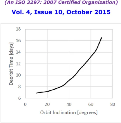
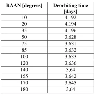
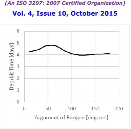
used within the ode45 solver, the integration time was considered to be 1 year, with a time step of 5 seconds. An aluminum electromagnetic tether of 20 km length was initially considered while the mass of the whole system (upper stage with electromagnetic tether and tether release mechanism) was taken to be 1000 kg. In Tables 3 – 8 and Figures 3 – 8 the deorbit times are shown with respect to the variation of the mass of the upper-stage, the initial orbital elements at end of mission and the length of the tether. While initial altitude, upper-stage mass, orbital inclination and tether length significantly affect the deorbit times, the RAAN and argument of periapsis variation have no observable influence over the deorbit efficiency.

Parameter Name Value for the Moon Value for the Sun Unit of measure

Eccentricity 0.0549 0.0167 n/a

Semi-major Axis 0.3855e+6 149.6+6 Km

Inclination 28.58 23.4 Degrees

Argument of periapsis 318.15 102.947 Degrees

Argument of ascending node 125.08 -11.26 Degrees

True anomaly at t0 169 0 Degrees

Table 2: Initial orbital elements of the Moon and the Sun

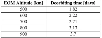
EOM Altitude [km] Deorbiting time [days]

500 1.82

600 2.22

700 2.71

800 3.13

(12)

1000 4.22

1100 4.9

1200 5.45

1300 6.22

1400 6.87

1500 7.76

1600 8.54

1700 9.26

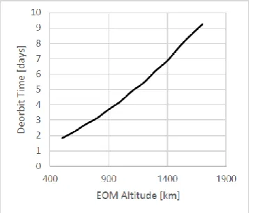
Table 3: Deorbiting time with EOM altitude variation

Figure 3: Graphic of Deorbiting time with EOM Altitude variance

Orbital inclination [degrees]

Deorbiting time [days]

10 6,89

15 7,05

20 7,18

25 7,46

30 7,81

35 8,25

40 9,08

45 9,88

50 11,03

55 12,04

60 13,18

65 14,41

70 16,53

(13)

Figure 4:Graph of Deorbiting time with Orbital Inclination variation

Spacecraft mass [kg] Deorbiting time [days]

1300 8.33

1400 8.85

1500 9.38

1600 9.9

1700 10.37

1800 10.84

1900 11.3

2000 11.83

Table 5: Deorbiting time with Spacecraft mass variation

(14)

RAAN [degrees] Deorbiting time [days]

10 4,192

20 4,194

35 4,196

50 3,628

75 3,631

85 3,632

100 3,633

120 3,636

140 3,64

155 3,642

170 3,645

180 3,64

Table 6: Deorbiting time with RAAN variation

Figure 6: Graph of Deorbiting time with RAAN variation(Mupper-stage=1000 kg, Ltether=20 km, hEOM=1000 km; i=30 deg; Argument of periapsis= 1 deg; e=0.0000133)

Orbital argument of perigee [degrees]

Deorbiting time [days]

10 4,252

30 4,44

45 4,742

65 4,773

85 4,352

100 4,107

115 3,985

135 3,99

150 4,056

165 4,061

180 4,124

(15)

Figure 7: Graph of Deorbiting time with argument of perigee variation (Mupper-stage=1000 kg, Ltether=20 km, h=1000 km; i=30 deg; RAAN=1 deg; e=0.0000133)

Tether length [km] Deorbiting time [days]

10 7,48

20 3,88

30 2,66

40 2,04

50 1,64

60 1,37

70 1,17

80 1,04

90 0,91

100 0,83

Table 8: Deorbiting time with tether length variation

(16)

IX. CONCLUSIONS

The results presented in the last chapter conclude the efficiency of the electromagnetic tether deorbit device for an upper-stage in LEO at EOM, having reduced theoretically the deorbit time significantly, while taking in account the perturbations upon the upper-stage’s deorbit trajectory for a more realistic deorbit scenario.The simulations done with variance of the orbital elements, upper-stage mass and electromagnetic tether length have shown significant influence in deorbit time. Further improvements of the numerical simulations code and electromagnetic tether device analysis include taking into account of the influence of different tether materials and architecture higher numerical simulation accuracies and simulations which show how the orbital elements vary during the upper-stage deorbit.

REFERENCES

1. Hildreth AS, Arnold A, “Threats to U.S. National Security Interests in Space: Orbital Debris Mitigation and Removal”, January, 2014.

2. Liou JC,“USA Space Debris Environment, Operations, and Measurement Updates”, 52nd Session of the Scientific and Technical Subcommittee Committee on the Peaceful Uses of Outer Space, United Nations, 2-13, February, 2015.

3. Matney M, “The Challenge of Orbital Debris”, National Aeronautics and Space Administration, 2014.

4. NASA, “Orbital Debris”, Quarterly News, International Space Station Performs Fourth and Fifth Debris Avoidance Maneuvers, 19:7, January, 2015.

5. NASA, “Orbital Debris”, Quarterly News, 11: 3, October, 2007.

6. Cosmo ML, Lorenzini EC, “Tethers in Space Handbook”, Third edition, Smithsonian Astrophysical Observatory, Cambridge, Massachusetts, USA, 1997.

7. Forward RL, “Electrodynamic Drag Terminator Tether”, Appendix K, Final Report on NAS8-40690, July, 1996.

8. Barcelo B, Sobel E, “Space Tethers: Applications and Implementations”, PKA-SB07, February, 2007.

9. Pardini C, Hanada T, Krisko PH, “Benefits and Risks of Using ElectrodynamicsTethers to De-orbit Spacecraft”, IAC-06-B6.2.10, 64: 571-588, 2009.