Estimation of critical streamflow discharge level using nonparametric quantile regression model

ESTIMATION OF CRITICAL STREAMFLOW DISCHARGE

LEVEL USING NONPARAMETRIC QUANTILE

REGRESSION MODEL

Dr. Francis Kiarie

PhD, Department of Management

Science, Kenyatta University, P.O Box 43844-00100 Nairobi,

Kenya.

[email protected]

ABSTRACT

Various parametric models have been designed to analyze volatility in river flow time series data. For maximum likelihood estimation these parametric methods assumes a known conditional distribution. This paper considers the problem of nonparametric estimation of critical streamflow discharge levels of a river regime based on quantile regression methodology of Koenker and Basset (1978).In particular, the paper demonstrates the use of kernel estimators for conditional quantiles resulting from a kernel estimation of conditional distribution function. It is finally proved that the estimate of the nonparametric quantile function is consistent and asymptotically normally distributed and under suitable conditions, the estimator converges uniformly with an appropriate rate.

Key words

:

Conditional quantile, kernel estimate, quantileautoregression, consistency, asymptotic normality, critical discharge level.

1.

INTRODUCTION

Globally, floods impact an estimated 520+ million people per year , resulting in estimates of up to 25,000 annual deaths, extensive homelessness, disaster-induced diseases, crop and livestock damage and other serious harm (UNU, 2004). One way of reducing losses due to floods is by use of flood early warning systems (FEWS). Such a system consists of streamflow monitoring and forecasting as well as public information system. Various methods are employed in hydrological stream flow monitoring and forecasting. For hydrological applications, models are usually based on regression relationships derived from paired catchment and catchment treatment experiments,Muthusi (2004).

The conventional method to estimate the conditional distribution function F (Yt|Xt) is to assume that Yt|Xt follows a particular distribution and then estimate its parameters. However, such specification may lead to wrong inferences and therefore, in this paper, we focus on quantile regression methodology introduced in Koenker and Basset (1978). This is a flexible method that requires no strict assumptions on moments and distribution of the underlying process. Instead of assuming that m(X) is a conditional mean, it is assumed to be θ-th conditional quantile and denoted as mθ(Xt).

In this paper, i use nonparametric approach to model mθ(Xt). I first estimate, non-parametrically, the conditional distribution of Yt given Xt and then invert it at θ- level of probability to get conditional θ-thquantile estimate as in Franke and Mwita (2003).

2.

THE STUDY MODEL (CRITICAL STREAMFLOW DISCHARGE LEVEL)

Assume that the underlying hydrological process of interest is of the form

Yt = mθ (Xt) + et. (2.1)

Franke and Mwita (2003) and Mwita (2005) for more details.

If we choose Xt = ( Yt-1,…….,Yt-d, Ut-1) where the random vector Ut consists of observations from other time series such as soil moisture budget(SMB), precipitation, evapotranspiration, El Nino Southern Oscillations( ENSO), Pacific Decadal Oscillations(PDO), then model (2.1) would become a quantile autoregressive model with exogenous components.

2.1

Estimation of critical streamflow discharge level

We consider the model (2.1), and define a true conditional distribution function Fx(y) of Yt given Xt = x as

Fx(y) = P(Yt ≤ y │Xt = x) = E[It,y│ Xt = x] (2.2)

where It,y = I{Yt ≤y} is an indicator function with Pr(Yt≤y|Xt = x ) = 1 and 0 otherwise.

For any θ  (0, 1), we define the true critical streamflow discharge level as

mθ(x)= inf{ y R│Fx(y) ≥ θ } (2.3)

The distribution function in (2.2) can be estimated by the Nadaraya (1964) and Watson (1964) estimator as





 



n

t 1 h t

y t, t n

1

t h

x

)

X

-(x

K

)I

X

-(x

K

(y)

F

ˆ

(2.4)

where K(u) is a d-dimensional kernel and Kh(u) = h-d K(u/h) is the rescaled kernel, see Franke and Mwita (2003) and Mwita(2005).Therefore the kernel estimator for the critical streamflow discharge level is given by

)

(

F

ˆ

}

(y)

F

ˆ

|

inf{R

(x)

m

ˆ

_



_x







_x-1



(2.5)

(y)

Fˆ

function

on

distributi

the

of

inverse

d

generalize

usual

the

)denotes

(

Fˆ

where

x

1

-x



_{which is a pure jump function of y.}

2.2

Asymptotic normality

Assume that the time series (Yt,Xt) satisfies α-mixing conditions. According to Masry and Tjostheim (1995, 1997), both ARCH processes and nonlinear additive autoregressive models with exogenous variables are stationary and α-mixing under some mild conditions. As Franke and Mwita (2003) demonstrated, if we choose Xt = Yt-d in (2.1) and assuming the time series Yt is α -mixing, we get an example of a quantile autoregressive process for which (Yt,Xt) and It,y in (2.4) are α -mixing as well.

The following assumptions are necessary for proving asymptotic normality of

(x)

m

ˆ

_

Henceforth, g (x) denotes the stationary probability density of Xt at point x.

(A1)For all uR

(i) K (u) ≥ 0

(ii) K is Lipschitz continuous i.e. │K(u)- K(v)│≤ Ck│u - v│,for all Ck,u,vR and Ck>0 (iii) │K(u) │≤ K∞ , with K∞ being a constant

(iv) ∫K(u)du = 1, ∫uK(u)du = 0 and ∫║ u ║ 2 k(u)du < ∞ (A2) For all y,x satisfying 0 <Fx(y) <1 , g(x) > 0

(i) Fx(y)and g(x) are twice continuously differentiable and bounded in y,x (ii) fx(mθ(x)) > 0, for all x.

(A3) The process (Yt, Xt) is stationary and α- mixing with mixing coefficients satisfying α(s) = O(s-(2 + δ) ) for some δ >0, n≥ 1, and {sn }is an increasing sequence of positive integers.

can be found in Franke and Mwita (2003).

Here, we only state the theorems.

proofs their and (x), mˆ of properties normality

asymptotic and

y consistenc

Theorem 3.1

Assume that (A1)- (A3) hold. As n → ∞, let the sequence of bandwidths h> 0 converge to 0 such that nhd → ∞. Then

)

(

(x)

m

ˆ

,

consistent

is

estimator

quantile

l

conditiona

the

_





p

m

_

x

that is

(Y)

f

B(Y)

-(y)

B

where

)

O(h

(x))

(m

B

h

(x)

m

-(x)]

m

E[

x m 2 m

2







_

 

ˆ

(2.6) Further if, the bandwidths are chosen such that nhd+4 is either 1 or converges to 0, then

normal,

ally

asymptotic

is

(x)

m

ˆ

_





_



















))

(

(

)

(

ˆ

(

,

0

))

(

(

)

(

)

(

ˆ

2 ₂

x

m

f

x

m

V

N

x

m

B

h

x

m

x

m

h

n

x D m d    (2.7) where , B(y) and V2(y) are the bias and variance expansion for the conditional distribution estimator in (2.4)

2.3

Uniform consistency and uniform convergence

For uniform consistency and uniform convergence of the quantile autoregressive estimate, Franke and Mwita(2003) first establishes the uniform consistency of the Nadaraya-Watson kernel estimate (2.4). For this purpose, the following conditions are imposed.

(B1) for some compact set G, there are ε>0, γ >0, such that g(x) ≥ γ for all x in the ε-neighborhood{x;║x-u║< ε for some u G} of G.

(B2) (Yt,Xt)isstationary and α-mixingwithmixing coefficients α(n), n≥ 1, and there is an increasing sequence sn, n≥ 1, of positive integers such that for some finite A

(n/sn) α 2sn/(3n)(sn) ≤ A, 1≤ sn≤ n/2 for all n≥1.

Uniform consistency and uniform rate of convergence properties of the estimator under the regularity conditions in Franke and Mwita, (2003) are given in Theorem 3.2.

Theorem 3.2

Assume (A1), (A2),(B1), and (B2). If, as n→ ∞,the bandwidthh→0such that







1

)

log

(

ˆ

_nh

_s

_n

S

_n d _n

then (3.2.4) is uniformly consistent on G in the strong sense. That is, forxG

0

|

)

(

)

(

ˆ

|







F

y

F

y

sup

_{x x}

G

x _a.s

2.4

Summary

In this section, we have shown that the estimate of our nonparametric quantile function is consistent and asymptotically normally distributed, and under suitable conditions, the estimator converges uniformly with an appropriate rate. The asymptotic normality property is used to construct the required confidence intervals for our estimator. These are strong properties that significantly imply sufficiency of our estimator is accurate estimation of the critical streamflow discharge level.

3.

REAL DATA RESULTS

The application of our estimator was performed with data from the gauge at River Nyando, in Western Kenya, (River Station No. IGD03) in the wider Nyando Basin, located at

35.2 oE longitude and -0.1oS latitude and covering an area of 3,587 km2. The drainage area downstream of the outlet of the catchment (IGD03) was found to accommodate all the discharge in the river channel. Flooding is experienced starting from Ahero plains, down to Lake Victoria through KUSA swamps. For this reason, monthly maximum streamflow data from gauging station IGD03 for the period 1970 – 1997 was used for calibrating the model. Also, the twenty-seven year period was considered long enough to capture diverse weather conditions, thus making the model to be a good representative of the basin.

Figure 3.1 Daily streamflow discharges for River Nyando (1970 – 1997) Station (IGD03)

Considering the critical streamflow discharge level to be our target variable, we first present hydrograph for monthly maximum streamflow for the period 1970 – 1997 in Figure 3.2.

Figure 3.2 Monthly maximum streamflow discharges for River Nyando (1970 – 1997) for Station (IGD03)

The hydrograph of figure 5.2 shows that the river pattern of low flows, peak flows and extremely high flows is preserved by the monthly maximum streamflow time series of our ground station gauging data.

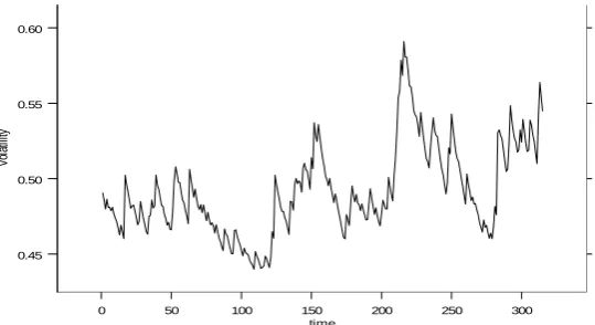
Figure 3.3 gives the volatility of the monthly maximum streamflow discharges. The hydrograph of these deviations depict the turbulence experienced by the Nyando River regime with an observable increase in trend.

1000 3000 5000 7000 9000

Days 0

100 200 300

R

iv

er

Fl

ow

0 50 100 150 200 250 300

Time 0

100 200 300

M

a

x

Fl

o

w

0 50 100 150 200 250 300

time 0.45

0.50 0.55 0.60

Vo

la

til

Figures 3.4 gives the monthly maximum streamflow discharge levels together with 0.95 and 0.99 conditional quantiles respectively.

Figure 3.4 Monthly maximum streamflow discharges with 0.95 and 0.99 quantiles.

The dotted curve represents the 0.95 conditional quantile while the dashed curve represents the 0.99 conditional quantile. Streamflow discharge levels above the 0.95-quantile curve represent critical streamflow discharge levels responsible for flood inundations at 95% confidence level. Such a level calls for some site-specific operational instructions to be issued by authorities monitoring the river catchment. The instructions may include shutting of floodgates and other engineering measures. Discharges above the 0.99 quantile curve represent extreme river flow levels. Such levels call for flood control teams to respond to imminent flood conditions and operate a warning system for the public as well as industries.

3.1

Model validation

To demonstrate that the study model produced good estimates, a model validity test using the Basler Amplel method of Backtesting was performed. This method is mainly applied in financial modeling. However, its basic principles do apply to other applications as well.

The Basler Ampel method suggests that we define a Bernoulli- distributed series of random variables Bi, such that

Bi = 1 if Yi>mθ (xi) or Bi = 0 if Yi<mθ(xi) i{1,2,……..,n} where n is the number of backtesting points. Yi is the streamflow discharge level for the i-th month. mθ(xi) is the

i-th month θ-th quantile level.This number is usually set at 250 or 500, but can be selected arbitrarily.

Using this model validation method, the study model was tested using a sample of size 250 data points. At both 99% and 95% confidence levels, the model results (4 data points at 99% and 16 data points at 95%) lied within the green zone of acceptance. Consequently, the study modelwas considered adequate in the estimations of critical stream flow discharge levels.

4.

REFERENCES

[1] Abberger, K. (1997). Quantile smoothing in Financial Time Series. Statistical papers Vol38, 125-148.

[2] Acreman, M. (1994). The Role of Artificial Flooding in Integrated Development of River basins in Africa. Journal of Hydrology, Vol78, 23-39.

[3] Box, G.E.P. and Jenkins, G.M. (1976). Time Series Analysis: Forecasting and Control. J. Clim., Vol14, 2105-2128.

[4] East African Standard, (15th May, 2003). http://www.eastandard.net/

[5] Franke, J. and Mwita, P. (2003). Nonparametric estimates for Conditional Quantiles of Time Series. Report in Economic Mathematics, Nr 87. Technical University of Kaiserslautern.

[6] Goswami, D.C. (2001). Flood Forecasting in the Brahmaputra River, India: ACase study, Department of Environmental science, Nr 222. Guahati University, Guahati-781014 Assam, India.

[7] Hardle, W. (1989). Applied nonparametric regression. Cambridge University press, Cambridge.

0 50 100 150 200 250 300

0

100

200

300

Monthly maximum Streamflow discharge with 0.95 and 0.99 Quantile

0 50 100 150 200 250 300

time

0

100

200

300

R

iv

e

rF

lo

[9] Jain, S. and Lall, U. (2001). Floods in a changing climate: Does the past represent the future? Water Resour. Res.,Vol37(12), 3193-3205.

[10] Japan International Co-operation Agency (JICA) (1992). Lake Victoria Basin Catchment Development. River Profile StudiesVol1.

[11] Koenker, R. and Bassett, G. (1978). Regression Quantiles. EconometricaVol46, 33-50.

[12] Kongo, V.M. (2001). Development of a Simulative Computerized Flood Warning System for River Nyando Flood Plain in Kenya. Msc Thesis, University of Dar es Salaam, Tanzania.

[13] Masry E., and Tjostheim, O. (1995). Nonparametric Estimation and Identification of Nonlinear ARCH time series: Strong convergence and asymptotic normality. Econometric Theory Vol. 11,258-289.

[14] Masry, E., and Tjostheim, O. (1997). Additive nonlinear ARX time series and projection estimates. Econometric Theory Vol. 13,214-252

[15] Ministry of Environment and Natural Resources (MENR, 1980) Annual Report on Flood Control in Kano Plains. Report No. 55(1980).

[16] Muthusi, F.M. (2004). Evaluation of the USGS Streamflow Model for Flood Simulation. M.Sc Thesis, Jomo Kenyatta University of Agriculture and Technology, Kenya.

[17] Mwita, P. (2003). Semi-parametric Estimation of Conditional Quantiles for Time Series with Application in Finance. PhD Thesis, University of Kaiserslautern, Germany.

[18] Mwita, P. (2005). On conditional scale function: Estimate and asymptotic properties. African Diaspora Journal of MathematicsVol2(2). In press.

[19] Nadaraya, E. A. (1964). On estimating regression. Theory Probab. Appl. Vol9, 141-142.

[20] Njogu, A.K. (2000). An integrated River Basin Planning Approach – Nyando Case Study in Kenya. Proceedings of the 1st WARFSA/Water Net Symposium on Sustainable Use of Water Resources; University of Zimbabwe, 1- 2 November 2000.

[21] Office for the Co-ordination of Humanitarian Affairs (OCHA) of the UN, (2002, May, 13). Situation Report No. 1, Kenya – Floods.

[22] Openshaw, S., Dougherty, M., Corne, S., See,.L (1997). Some initial experiments with neural network models of flood forecasting on the River Ouse. Proceedings of the 2nd annual conference of GeoComputation, University of Otago, New Zealand, 26-29 August 1997.

[23] Ruppert,D., Sheather,S.J and Wand, M.P.(1995). An effective bandwidth selector for local least squares regression. J. Amer. Statist. Assoc.,Vol90, 1257-1270.

[24] Sankarasubramanian, A. and Upman, L. (2003). Flood quantiles in a changing climate: seasonal forecasts and casual relations. Water resources research,Vol39 (5),1-12.

[25] Scudder, G. (1980). River Basin Development and Local Initiative in African Savanna Environments. Academic Press, London.

[26] Stronsaka, K. and Borowicz, A.(2002). MIKE II as Flood Management and Flood Forecasting Tool for the Odra River, Poland. Journal ofHydrology, Vol15, 65-70

[27] Tukey, J.W (1977). Exploratory data analysis. Theory prob. Appl.Vol10, 200-205.

[28] United Nations University (UNU) (2004). The June- August newsletter of United Nations University and its international network of research and training centers/programmes. Accessed from http://www.update.unu.edu/issue322.htm .

[29] Vertessy, R.A., T.J. Hatton, P.J. O’shaughnessy (1993). Predicting Water Yield From a Mountain Ash Forest Catchment using Terrain Analysis Based Catchment Model. Journal ofHydrology, Vol150, 665-700.

[30] Watson, G. S. (1964). Smooth regression analysis. Sankya ser. A26, 359-372.

[31] Weiss, A. (1984). ARMA models with ARCH errors. Journal of Time SeriesAnalysis Vol.3, 129-143.

[32] Woolhiser, D.A. and D.L. Brakensiek (1982). Hydrological System Synthesis. ASAE Monograph No. 5, 3-16.

[33] Yakowitz, S.J. (1985). Markov Flow Models and the Flood warning Problem. Water Resources Research, Vol21,81-88.