Abstract. The DIRECT algorithm is a deterministic sampling method for bound constrained Lipschitz continuous optimization. We prove a subsequential convergence result for the DIRECT algorithm that quantifies some of the convergence observations in the literature. Our results apply to several variations on the original method, including one that will handle general constraints. We use techniques from nonsmooth analysis, and our framework is based on recent results for the MADS sampling algorithms.
Key words. DIRECT, Sampling Methods, Clarke derivative, Lipschitz Functions
AMS subject classifications. 65K05, 65K10
1. Introduction. The DIRECT (DIviding RECTangles) algorithm [19] is a determin-istic sampling method. The method is designed for bound constrained non-smooth problems in a small number of variables. Typical applications are engineering design problems, in which complicated simulators are used to construct the objective function [3–8, 16].
By a sampling method we mean that the progress of the optimization is governed only by evaluations of the objective function. No derivative information is needed. Unlike most classical direct search methods [21, 25] such as the Hooke-Jeeves [17], Nelder-Mead [22], implicit filtering [15, 20], or the variations [1, 2, 10] of the multidirectional search algorithm, DIRECT does not sample on a stencil about the current best point at any stage of the optimization, and is designed to perform a global search as the optimization progresses. DIRECT is a naturally parallel algorithm, in that a large number of calls to the objective function can be made simultaneously, and distributed to multiple processors.
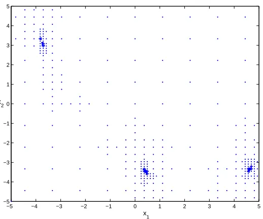
In the limit, DIRECT will sample a dense grid of points in the feasible set. The behavior of the iteration in the early to middle phases is more important, however. The typical observations are that the sampling clusters near local optima [5–8, 12]. Figure 1.1 is an example of such clustering. The figure is a plot of the 521 sample points from the first first 28 iterations of DIRECT as as applied to the Branin function, a test problem used in [19].
The purpose of this paper is to analyze the behavior of DIRECT by showing that certain subsequences of the sample points converge to points that satisfy the necessary conditions for optimality in the sense of Clarke [9]. We do this using the framework from [1], in which the authors design a sampling algorithm with a very rich set of search directions. The richness of that set allows them to extend the results of [2] to show that all cluster points of the iterations for the new method satisfy certain nonsmooth necessary conditions for optimality. In this paper we observe that DIRECT, which is not based on search directions at all, can be analyzed with these techniques.
∗Version of July 14, 2004.
† North Carolina State University, Center for Research in Scientific Computation and Department of
Mathematics, Box 8205, Raleigh, N. C. 27695-8205, USA ([email protected], Tim [email protected]). This research was supported in part by National Science Foundation grants DMS-0070641, DMS-0112542, and DMS-0209695.
−5 −4 −3 −2 −1 0 1 2 3 4 5 −5
−4 −3 −2 −1 0 1 2 3 4 5
x
1
x
2
Fig. 1.1. Branin function example
We consider a bound-constrained optimization problem,
min
x∈Ωf(x), where f :R
N →
R, (1.1)
where
Ω =©
x∈RN
:l ≤x≤uª
.
and f is Lipschitz continuous on Ω.
DIRECT begins by scaling the domain, Ω, to the unit hypercube. This transforma-tion has no impact on the results, simplifies the descriptransforma-tion and analysis, and allows the implementation to pre-compute and store common values used repeatedly in calculations, thereby reducing the run-time of the algorithm. Thus, for the remainder of this paper, we will assume that
Ω = ©
x∈RN : 0≤x
i ≤1
ª
.
DIRECT’s sample points are centers of hyperrectangles. In each iteration, new hyper-rectangles are formed by dividing old ones, and then the function is sampled at the centers of the new hyperrectangles. We refer to a divide-sample pair as an iteration. In the first, or division phase of an iteration, DIRECT identifies hyperrectangles that show the most potential to contain good, unsampled points. The second or sampling phase is to sample f
at the centers of the newly created hyperrectangles. DIRECT typically terminates when a user-supplied budget of function evaluations is exhausted.
In this next section, we outline the original DIRECT algorithm, and discuss several modifications that have been done. Our results apply to very general constraints, if one takes the approach in [5, 6] of assigning an artificial value to an infeasible point.
we review some basic ideas from nonsmooth analysis and state and prove our convergence results for the case of simple bound constraints. In § 3.3, we use more general concepts from [1, 2, 9] to prove the result for general constraints.
2. Description of DIRECT. DIRECT initiates its search by sampling the objective function at the center of Ω. The entire domain is treated as the first hyperrectangle, which DIRECT identifies as potentially optimal and divides.
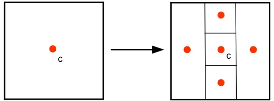
DIRECT divides a potentially optimal hyperrectangle by trisecting the longest coordinate directions of the hyperrectangle. For example, in the first iteration when the hypercube Ω is potentially optimal, all directions are long, andDIRECTdivides in every direction. Figure 2.1 illustrates this process.
The order in which sides are divided is important; the right-hand side of Figure 2.1 would look different had the vertical side of the rectangle been divided first. DIRECT employs a simple heuristic to determine the order in which long sides are divided. This process is explained in Table 2.1.
c c
Fig. 2.1. Two dimensional example of division by DIRECT
Table 2.1
Division of a hyperrectangle hwith centerc
1: Let h be a potentially optimal hyperrectangle with center c. 1: Let ξ be the maximal side length ofh.
2: Let I be the set of coordinate directions corresponding to sides of h with length ξ. 3: Evaluate the objective function at the points c± 13ξei,
for all i∈I, whereei is the ith unit vector
4: Let wi = min
©
f(c± 1 3ξei)
ª
5: Divide the hyperrectangle containing cinto thirds along the dimensions in I, starting with the dimension with smallest wi and continuing to the dimension
with the largest wi.
into groups of the same size, and considers subdividing hyperrectangles in the subgroups with the smallest value of f at the center. Not all such hyperrectangles are divided; an es-timate of the Lipshitz constant off is used to complete the selection. The formal definition from [19] is
Definition 2.1. Let H be the set of hyperrectangles created by DIRECT after k
itera-tions, and let fmin be the best value of the objective function found so far. A hyperrectangle
R∈ H with centercR and size αR is said to be potentially optimal if there exists Kˆ such that
f(cR)−Kαˆ R≤f(cT)−Kαˆ T, for all T ∈ H (2.1)
f(cR)−Kαˆ R≤fmin−²|fmin|. (2.2)
In (2.2), ² ≥ 0 is a “balance parameter” which provides the user control of the balance between local and global search.
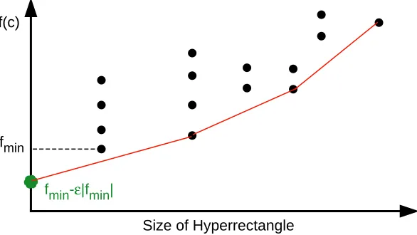
Figure 2.2 illustrates the definition. Each point on the graph represents a subgroup of hyperrectangles having equal sizes (horizontal axis) and equal function values at the centers (vertical axis). The hyperrectangles represented by points on the lower right convex hull of this graph satisfy Equations 2.1 and 2.2, and thus are potentially optimal. Note the role of the balance parameter.
fmin
fmin-ε|fmin|
f(c)
Size of Hyperrectangle
Fig. 2.2. Hyperrectangles on the piecewise linear curve are potentially optimal
In choosing the hyperrectangles from the lower right convex hull of Figure 2.2, the local and global search characteristics of DIRECT are illustrated. Hyperrectangles with low objective function values are inclined to fall on the convex hull of the set, as are (relatively) large hyperrectangles. One of the largest hyperrectangles will always be chosen for division [12, 19].
The parameter ² was introduced in [19] to balance the local and global search. In Figure 2.2, we see the effects of using the balance parameter. The point (0, fmin−²|fmin|)
In the original implementation of DIRECT, the size of a hyperrectangle, αR, is defined
to be the distance from the center to a corner. In [13], a modified version of DIRECT is derived which measures hyperrectangles by their longest side. In this way, the groups of hyperrectangles are larger, and consequently the iteration places a stronger emphasis on the value of the objective function at the center of a hyperrectangle. This tends to bias the search locally, as reported in [13].
In [16], the idea of potentially optimal hyperrectangles is discarded, and the imple-mentation described divides hyperrectangles with the lowest function value from each size grouping. This is an aggressive version of DIRECT that was designed to exploit massive parallelism.
2.1. DIRECT’s Grid. DIRECT samples from a dense set of points in Ω [12]
S = ½
x|x=
N
X
i=1
2ni+ 1
2·3ki ei ¾
where ei is the ith coordinate vector, ki ≥0, and 0≤ni ≤2·3ki −1.
We let Sk be the set of points that have been sampled after k iterations, and letBk, the
set of best points be
Bk ={x∈ Sk|f(x)≤f(z) for all z ∈ Sk }.
Since at least one of the largest hyperrectangles will be potentially optimal at each iteration [19], any given in point S will be sampled after finitely many iterations, i. e.
S =∪kSk.
Hence, DIRECT is, in the limit, an exhaustive search and will, iff is continuous, find an arbitrarily accurate approximation to the global minimum [24]. DIRECT has more structure than this, however.
Let B be the set of best points
B=∪kBk.
The objective of this paper is to study the cluster points of B.
2.2. General Constraints. Bound constraints are part of DIRECT’s sampling strat-egy, and are incorporated automatically into the optimization. DIRECT can address more general constraints by assigning an artificial value to the objective function at an infeasible point. An obvious way to do this is to assign a large value to such a point. However, such an approach will bias the search away from the boundary of the feasible region. If the solution is on or near that boundary, this approach will significantly degrade the performance of the algorithm.
we flag the point as infeasible, and assign a (relatively) large value to it. Otherwise, we assign an artificial value of f∗+δ|f∗|, where f∗ is the minimum value of f over the feasible
points in the larger hyperrectangle. In [14], δ = 10−6. This strategy, while non-trivial to
implement [14], does not bias the sampling away from the boundary of the feasible region. DIRECT makes no distinction between inequality constraints that are given directly as formulae and “hidden” constraints, which can only be detected when f fails to return a value.
We let D denote the feasible set. We will assume very little about the specific way in which artificial values are assigned to infeasible points. We will assume only that if z /∈ D, then we assign a function value to z that is larger than fmin, wherefmin is the current best
value of f, ie
Bk ⊂ D, for all k. (2.3)
3. Convergence Results: Simple Bound Constraints. In this section we state and prove a convergence result for the case of simple bound constraints. To do this we require a small subset of the results from [9] that were used in [1, 2]. The fully general results will require more of that machinery.
3.1. Results from Nonsmooth Analysis. In this section, we review the tools from nonsmooth analysis [9] that we will need to state and prove the result for simple bound constraints. Throughout we will assume thatf is a Lipschitz continuous real-valued function on X ⊂ RN. In the context of this paper, X = Ω if there are no constraints other than
simple bounds, and X =D if there are more general constraints.
Following [9, 18], we define the generalized directional derivative of f at x ∈ X in the direction v as
fo(x;d) = lim sup y→x, y∈X t↓0, y+tv∈X
f(y+td)−f(y)
t . (3.1)
We seek to show that if x∗ is a cluster point of B, then the necessary conditions for
optimality hold, i. e.
fo(x∗;v)≥0 (3.2)
for all v ∈TCl
Ω (x∗), the Clarke cone of directions pointing from x∗ into Ω.
The cone of directions is easy to describe if there are only simple bound constraints. If
x∈Ω, the Clarke tangent cone atx is
TCl
Ω (x) ={v ∈RN|x+tv∈Ω for all t >0 sufficiently small}.
3.2. Statement and Proof of the Convergence Theorem. The formal statement of our convergence result is
Theorem 3.1. Let f be Lipschitz continuous on Ω and let x∗ be any cluster point of
B. Then (3.2) holds.
Proof. We will show that (3.2) holds with an indirect proof. Assume that fo(x∗;v)<0
for some v ∈TCl
Ω (x∗). We will exhibit K and ∆>0 such that
inf
k≥Kdist(x
∗,B
contradicting the assumption that x∗ is a limit point of B.
Since fo(x∗;v)<0 and v ∈TCl
Ω (x∗), there is δ >0 such that
y∗ =x∗+δv∈Ω,
and f(y∗)< f(x∗).
Let Lf denote the Lipschitz constant off. Let
∆ = min ½
δ/2,f(x
∗)−f(x∗+δv)
2Lf
¾
(3.4)
and let
N ={x| kx−x∗k ≤∆} ∩Ω. (3.5)
For all x∈ N,
f(x)−f(y∗)≥f(x∗)−L
f∆−f(y∗)≥
f(x∗)−f(y∗)
2 >0. (3.6) Since S is dense in Ω, there is K >0 and ˆx∈ SK such that
kˆx−y∗k ≤∆/2,
and hence, for all x∈ N,
f(ˆx)≤f(y∗) +LF∆/2≤f(y∗) +
f(x∗)−f(y∗)
4 < f(x). (3.7)
Hence,
N ∩ Bk =∅
for all k ≥K, as asserted.
3.3. Convergence Results: General Constraints. In this section, we extend our nonsmooth results to a more general design space, D ⊂ Ω. Again, DIRECT attempts to minimize f over Ω, and assigns artificial values to any x6∈ D (that is, x∈ DC).
As we said in § 2.2, the only requirement on the artificial assignment heuristic is (2.3). Examples of such assignment strategies include the already discussed approach of [14], the barrier approach used in [1], a traditional penalty function approach [11], and others.
The strength of the results in this section are dependent upon assumptions about prop-erties of D at the cluster points of B, a fact first pointed out in [23]. Our analysis follows the program from [1].
We first define a hypertangent cone.
Definition 3.2. A vectorv ∈RN is said to be a hypertangent vector to the setD ⊂
RN
at the point x∈ D if there exists a scalar ² >0 such that
y+tw∈ D for all y∈ D ∩B²(x), w∈Be(v), and 0< t < ². (3.8)
The set of hypertangent vectors to D at x is called the hypertangent cone to D at x and is denoted by TH
If x∗ is a cluster point of B, then (3.2) holds for allv ∈TH
D(x∗).
Theorem 3.3. Let f be Lipschitz continuous on D and let x∗ be any cluster point of
B. Then fo(x∗;v)≥0 for all v ∈TH
D(x ∗).
Proof. The proof is a simple extension of the proof of Theorem 3.1. Assume that
fo(x∗;v)<0 for somev ∈TH
D(x∗). Then, there exists 0< δ < ² such that
y∗ =x∗+δv∈ D,
and f(y∗)< f(x∗).
Define ∆ and N by (3.4) and (3.5), and letDC denote the complement of D. We have
¡
N ∩ DC¢
∩ Bk=∅, (3.9)
because Bk⊂ D.
Since S is dense in Ω, it follows that there exists K and ˆx = x∗ +tw ∈ S
K, for some
0< t≤δ, and w∈B²(v). Since v ∈TDH(x∗) it follows that ˆx∈ D. Furthermore, we choose
ˆ
x so thatkw−vk and |t−δ| are small enough to ensure that
kˆx−y∗k=ktw−δvk ≤∆/2.
As already shown in (3.6) and (3.7), f(ˆx)< f(x) for all x∈ N ∩ D, so
(N ∩ D)∩ Bk =∅, (3.10)
and thus (from (3.9) and (3.10)),
N ∩ Bk =∅,
for all k ≥K, which proves our assertion.
Theorem 3.3 differs from Theorem 3.1 in that the set of directions for which (3.2) holds are not, in general, the same. In the case of simple bound constraints,TH
D(x∗) is non-empty,
and its closure is TCl
D (x), so if (3.2) holds for all v ∈ TDH(x∗), it holds by continuity for all
v ∈TCl
D (x). This is not so in the general case. To explore the new assumptions necessary to
we follow [1], and use the more general definitions of the Clarke and contingent cones [9,18,23] for this purpose.
Definition 3.4. A vector v ∈ RN is said to be a Clarke tangent vector to the set
D ⊂RN at the point x in the closure of D if for every sequence {y
k} of elements of D that converges tox and for every sequence of positive real numbers {tk} converging to zero, there exists a sequence of vectors {wk} converging to v such that yk+tkwk ∈ D. The set TDCl(x)
of all Clarke tangent vectors to D at x is called the Clarke tangent cone to D at x.
Definition 3.5. A vector v ∈RN is said to be a tangent vector to the set D ⊂RN at
the point xin the closure of D if there exists a sequence{yk}of elements of D that converges to x and a sequence of positive real numbers {λk} for which v = limkλk(yk−x). The set
TCo
D (x) of all tangent vectors toD atxis called the contingent cone (or sequential Bouligand
tangent cone) to D at x.
The three cones are nested [1],
TDH(x)⊆T
Cl
D (x)⊆T
Co
They also note that, if TCl
D (x) = TDCo(x), the set D is said to be regular at x.
Our next two results state the necessary assumptions to show that DIRECT finds Clarke and contingent stationary points.
Theorem 3.6. Let x∗ be a cluster point ofB. If TH
D(x∗)6=∅, then fo(x∗;v)≥0for all
v ∈TCl
D (x∗).
Proof. By Theorem 3.3, fo(x∗;w) ≥ 0 for all w ∈ TH
D(x∗). If TDH(x∗) is non-empty,
then [1],
fo(ˆx;v) = lim w→v w∈TH
D(ˆx)
fo(ˆx;w)≥0,
as asserted.
We conclude by extending our results to differentiable functions. We first state a simple observation (also made for MADS methods in [1]) that if the setDis regular (i. e. TCl
D (x) =
TCo
D (x)) at x∗, then cluster points of B are stationary with respect to the contingent cone.
Corollary 3.7. Let x∗ be a cluster point of B. If TH
D(x∗)6=∅, and if D is regular at
x∗, then fo(x∗;v)≥0 for all v ∈TCo
D (x∗).
Our final result extends Corollary 3.7. If we assume strict differentiability of f, then we can state the constraint qualifications needed to show that cluster points of B are KKT points.
Theorem 3.8. Let f be strictly differentiable, and let x∗ be a cluster point of B. If
TH
D(x∗) 6= ∅, and if D is regular at x∗, then x∗ is a contingent KKT stationary point of f
over D.
Proof. As pointed out in [1,9], strict differentiability off atx∗ implies that∇f(x∗)Tv =
fo(x∗;v) for all v ∈TCo
D (x∗). Thus, it follows from the previous corollary that−∇f(x∗)Tv ≤
0 for all v in the contingent cone.
Acknowledgments. The authors are very grateful to John Dennis and Evin Kramer for their thoughtful comments on a preliminary version of this paper.
REFERENCES
[1] C. Audet and J. E. Dennis, Mesh adaptive direct search algorithms for constrained optimization, Tech. Rep. TR04-02, Department of Computational and Applied Mathematics, Rice Univeristy, 2004.
[2] C. Audet and J. D. Jr., Analysis of generalized pattern searches, SIAM J. Optim., 13 (2003), pp. 889–903.
[3] C. A. Baker, L. T. Watson, B. Grossman, R. T. Haftka, and W. H. Mason,Parallel global aircraft configuration design space exploration. preprint, 1999.
[4] C. A. Baker, L. T. Watson, B. Grossman, W. H. Mason, S. E. Cox, and R. T. Haftka,
Study of a global design space exploration method for aerospace vehicles. preprint, 1999.
[5] R. Carter, J. Gablonsky, A. Patrick, C. Kelley, and O. Eslinger,Algorithms for nosiy prob-lems in gas transmission pipeline optimization, Optimization and Engineering, 2 (2001), pp. 139– 157.
[6] R. G. Carter,Compressor station optimization - computational accuracy and speed, 1996. Proceed-ings of the Pipeline Simulation Interest Group, Twenty-Eighth Annual Meeting, San Francisco CA, Paper number PSIG-9605.
[8] R. G. Carter, W. W. Schroeder, and T. D. Harbick,Some causes and effect of discontinuities in modeling and optimizing gas transmission networks, 1993. Proceedings of the Pipeline Simulation Interest Group, Pittsburg PA, Paper number PSIG-9308.
[9] F. Clarke, Optimization and Nonsmooth Analysis, Canadien Mathematical Society Series of Mono-graphs and Advanced Texts, Wiley-Interscience, New York, 1983.
[10] J. E. Dennis and V. Torczon, Direct search methods on parallel machines, SIAM J. Optim., 1 (1991), pp. 448 – 474.
[11] R. Fletcher,Practical Methods of Optimization, John Wiley and Sons, New York, second ed., 1987. [12] J. Gablonsky, Modifications of the Direct Algorithm, PhD thesis, North Carolina State University,
2001.
[13] J. Gablonsky and C. Kelley, A locally-biased form of the direct algorithm, Journal of Global Optimization, 21 (2001), pp. 27–37.
[14] J. M. Gablonsky,DIRECT Version 2.0 User Guide, Tech. Rep. CRSC-TR01-08, Center for Research in Scientific Computation, North Carolina State University, April 2001.
[15] P. Gilmore and C. T. Kelley, An implicit filtering algorithm for optimization of functions with many local minima, SIAM J. Optim., 5 (1995), pp. 269–285.
[16] J. He, L. Watson, N. Ramakrishnan, C. Shaffer, A. Verstak, J. Jian, K. Bae, K. Bae, and W. Tranter,Dynamic data structures for a direct search algorithm, Computational Optimization and Applications, 23 (2002), pp. 5–25.
[17] R. Hooke and T. Jeeves, Direct search solution of numerical and statistical problems, Journal of the Association for Computing Machinery, 8 (1961), pp. 212–229.
[18] J. Jahn,Introduction to the Theory of Nonlinear Optimization, Springer, Berlin, 1994.
[19] D. Jones, C. Perttunen, and B. Stuckman, Lipschitzian optimization without the lipschitz con-stant, Journal of Optimization Theory and Application, 79 (1993), pp. 157–181.
[20] C. Kelley, Iterative Methods for Optimization, Frontiers in Applied Mathematics, SIAM, Philadel-phia, PA, first ed., 1999.
[21] T. Kolda, R. Lewis, and V. Torczon, Optimization by direct search: New perspective on some classical and modern methods, SIAM Review, 45 (2003), pp. 385–482.
[22] J. Nelder and R. Mead,A simplex method for function minimization, Comput. J., 7 (1965), pp. 308– 313.
[23] R. Rockafellar,Generalized directional derivatives and subgradients of nonconvex functions, Cana-dien Journal of Mathematics, 32 (1980), pp. 157–180.
[24] C. P. Stephens and W. Baritompa, Global optimization requires global information, J. Optim. Theory Appl., 96 (1998), pp. 575–588.