An approximate analysis of a bufferless NxN synchronous Clos ATM switch

(1)

An Approximate Analysis of a

Bufferless

N

x

N

Synchronous

Clos

ATM

Switch

Arne A. Nilsson

Fuyung Lai

Harry G. Perros

Center for Communications and Signal Procesing

Department of Electrical and Computer Engineering

Department of Computer Science

North Carolina State University

(2)

An Approximate Analysis of a Bufferless

NxN

Synchronous Clos ATM Switch

Arne A. Nilsson and Fuyung Lai

Center for Communications and Signal Processing

Department of Electrical and Computer Engineering

Raleigh, N.C. 27695-7914

Harry G. Perros

Department of Computer Science

Center for Communications and Signal Processing

Raleigh, N.C. 27695-8206

June 1990

Abstract

(3)

1

Introduction

The Asynchronous Transfer Mode(ATM) appears to be the most prorrusmg solution for broadband ISDN. ATM provides the means to transporting different types of highly bursty traffic such as voice, video and bulk files. It is based on the principle of packet switching, and all the packets(known as cells) have a fixed length of 53 bytes. Various types of architectures

have been proposed for an ATM switch. Most of these architectures are based on multi-stage interconnection networks. The switching elements in a multi-stage interconnection network may be buffered or unbuffered. In the unbuffered case, there may be buffers at the input ports of the switch, or at the output ports, or at both input and output ports. There have been several performance studies of such switch architectures (see for instance Oie, Suda, Masayuki, and Miyahara [1], Shaikh, Schwartz, and Szymanski

[2],

Hluchyj and Karol [3]). For the performa.nce analysis of switches with buffered switching elements see Yoon, Lee, and Liu

[4],

and the references within. Finally, we note that there is a different type of switch architecture based on the concept of the shared buffer. For further references, we refer the

reader

to IIuang and Knauer

[5],

and Devault, Cochennec, and Servel

[6].

In this paper, we consider a bufferless ATM switch with buffers at the input ports. The switch fabric is a Clos three-stage interconnection network. For this type of switch we construct an approximation algorithm under the assumption of bursty arrivals. The a.pproximate results were extensively validated against simulation data. We now proceed to describe the switch under study in detail.

2

Model description

Let us consider an N x N Clos cell switch, as shown in figure 1. There are three stages in the switch. At each stage, there are n or

VN

number of bufferless switching elements. Each switching element is an n xn crossbar switch. For each input buffer, there is a cell processor to handle the incoming cells. The cell processor is responsible for determining the output port of a cell and then transmitting the cell through the switch fabric.

(4)

slo~.

The retransmissions will continue until the cell is successfully transmitted through the switch.

o

o 0 0 [ } N-n+l

o n 0 0 n 0

t - - - I

.-0

0_

:

N n

1

-..[[il]-1

2 0

0 ₂

0 ₁ 0

-..[]]I]- 0

n 0

n

n+l _n+1

0

:[}

0

2n

o 0

2n

0

N

N-n+l~!!!!!!!!!!!!I:=:Z:::::::::~

o

figure 1: Synchronous N x N Clos ATM Switch.

The time required for a cell to pass through the switch fabric is equal to one slot time. It is assumed that each incoming line is slotted. The length of a slot is equal to a slot of the ATM switch. Each incoming line is not synchronized with the other incoming lines and with the switch. A cell that arrives at an idle cell processor in the middle of a slot of the ATM switch is not transmitted until the beginning of the next time slot of the ATM switch.

The arrival process to each input port of the ATM switch is modeled as a discrete time Interrupted Bernoulli Process(IBP).

Active Active ( p

I die 1 - q

(1)

(5)

active state arrivals occur in a Bernoulli fashion. In particular, if the process is in the idle state, then in the next time slot it remains in the idle state with probability q or it will change to the active state with probability 1-q. Likewise, if it is in the active state, then in the next slot it will remain in the same state with probability p or it will change to idle with proability 1-p. Those transition rates are shown in ( 1). If the input process is in the active state, a slot will contain a cell with proability a. Let

l

be the interarrival time of a cell and

t.

be the time interval from a slot in the idle slot to the time of the next arrival. Then,

l

is equal to 1 with probability pa if the process is in the active state in the next time slot and the slot is filled with a cell. If the process is in the active state in the next time slot and the slot is empty, from the memoryless property,

i

is equal to 1

+

i

with probability p(l - a). If the process changes to the idle state in the next time slot,

i

is equal to 1

+

{1

with probability 1 - p. t-1 is obtained using similar arguments and we get

i

{

1 ,pa

l+i ,p(l -

0:)

1

+

i1 ,1-P

{

1

+

i

1 ,q

1 , (1 - q)a

l+i ,(1 - q)(l - a)

(2)

(3)

Hence,

zpcc

+

zp{l - a)E{zf}

+

z{l - p)E{zt1_}

zqE{zt1

}

+

za(l - q)

+

z(l - q)(l - a)E{zt}

(4)

(5)

Let A( z) be the z-transform of the probability distribution of the interarrival time; i.e.

za[p+ z(l- p - q)]

(1 - a)(p

+

q - 1)z2 - [q

+

p(l - a)]z

+

1

(6)

From this z-transform we can obtain the mean interarrival time E(i) and the squared coef-ficient of variation of the interarrival time, C2 , as :

E{l} =

(2 -

p - q)

a{l - q)

Var(i)

[E(i)]2

1

+

a

((1 -

p)(3 -

q) _

2)

+

0 2

(1-

q)2

(2 -

p - q)2

(2 _

p _ q)2

(7)

(6)

If Q == 1, 02 is :

C2

= (1 - p)(p + q)

(2 -

p - q)2

(9)

In this paper, we present an approximation method for analyzing the performance of the ATM switch described above. In section 3, we obtain the probability that a cell will be successfully transmitted when it is launched through the switch. In section 4, we analyze the buffer in front of a cell processor as an IBP /Geo/l queue first with infinite capacity and then with finite capacity. We also give a simple approximation algorithm for analyzing the ATlVI switch. In section 5, the approximation results are compared against simulation for a 16 x 16 switch under a variety of traffic loads. Finally, conclusions are given in section 6.

3

Probability of success for transmission through the

Clos switch

In this section we extend the probability of success analysis of a crossbar switch [7, 8] to the Clos ATM switch. Let us consider a crossbar switch of size n xn. Assume that in each time slot a cell arrives at each input port independently with probability p and the destination of each cell is randomly selected. The probability that an incoming cell will be successfully transmitted to its destination output port , p~ ,is computed as follows:

(10)

(11) Another way to compute the success probability is the following. In a switching element, the probability that all n input lines will not select a specific output line is

(1

-2.

r

The probability that a particular output line is requested by any of the input lines is

1-

(1 -

2.t.

Thus, the expected number of busy output lines is n(1 - (1 -

;)n)

and the expected.number of input lines is tip, The average probability that an input line will be successfully connected to the destined output line of the crossbar switch is calculated as :

Expected number of busy output lines

Expected number of busy input lines

~

{[1 - (1 - ;

t] }

(7)

3.1

Sym

met ric input case

Let P be the utilization of each cell processor of the Clos ATM switch, or in another words, the probability that in each time slot a cell processor has a cell to transmit. Let N be the total number of independent input lines of the Clos ATM switch. Assume that the destination of a cell is uniformly selected. Let PI be the average output line utilization of a switching element in the 1st stage of the Clos ATM switch. From the assumption that there is no blocking in the 1st stage of the switch, we get

PI

==

P

(12)

Let P2 andP3 be the average output line utilizations of the switching element in the 2nd and

3rd stage of the switch given that each input line has PI, P2 probability of being busy. We have

(1

Pi_l)n

Pi

=

1 - - ---:;;,- i

==

2 and 3

(13)

The probability for a cell successfully passing through the Clos ATM switch ,1 - a ,is com-puted as

1-u Average number of busy output lines at the 3rd stage

Average number of busy input lines at the 1st stage

NP3

Np

P3

P

(14)

3.2

Asymmetric input case

Let Pi,i

==

1 · · ·N be the utilization of theith cell processor of the Clos ATM switch. Assume that in a time slot the ithinput line of the ATM switch has a cell to transmit with probability

Pi and the input cells are equally likely destined to the N outputs. The transmission at an input line is assumed to be independent of the other lines. Let p~l], p~2], p~3] be theitk output line utilizations of the switching elements in the 1st, the 2nd, and the 3rd stage of the Clos ATM switch. Following the assumption that there is no contention in the 1st stage of the switch, the average output line utilization in the 1st stage is computed as :

P~~+j

= ( .

f:

Pi)

In

(.1-1)n + l

k

==

0, ...,n - 1, j

==

1,2,· .. ,n

(15)

(8)

apply the analysis in crossbar switch to compute p~2J and p~3J,i= 1 ... N. We get

[2] _ in p~l]

Pkn+i- 1 -

II

(1--) k=O,· .. ,n-1, j=1,2,···,n (16)

(i-l)n+l n

and

[ ]3

II

in p.[2]

Pkn+i

==

1 - (1 _ _

20_)

(j-l)n+l n

k=O ..._" n - l

,

_{j=1,2,···,n} ₍₁₇₎

The probability for a cell successfully passing through the Clos ATM switch ,1 - (J", is com-puted as:

1-u

==

Average number of busy output lines at the 3rd stage Average number of busy input lines at the 1st stage

N ' " [3] L.J Pi i=l

N

LPi

i=l

(18)

4

Exact analysis of the IBP /Geo/l and IBP /Geo/l/K

queues

Let us consider a cell processor queue. It is obvious from the previous section that the total time it takes for the cell processor to transmit successfully a cell through the switch fabric is geometrically distributed with probability a . Therefore, a cell processor queue can be modeled by a discrete IBP /Geo/l/K queue. Customers are served in this queue in a FIFO manner. The IBP/Geo/l queue is a special case of the GI/Geo/1 queue which has

been already analyzed(see Hunter[9] ,chapter 9). It can be also shown that the GI

/Geo/l/

K

queue can be analyzed due to a duality with the Geo/GI

/1/

K queue. The dual of the

GI /Geo/l/K queue is constructed by looking at the flow of holes through the queue. The

GI distribution becomes the arrival distribution for the holes, and the Geo distribution

becomes their service distribution. In this case, it can be shown that the queue-length distribution in a GI /Geo/l/ K queue is equal to the distribution of the holes obtained by

analyzing a Geo/GI

/1/

K queue. Now, the queue-length distribution in the latter queue

is obtained by truncating the queue-length distribution in the Geo/GI/l queue. We note

that this approach requires that the resulting Geo/GI/1 queue is stable, which may not be

the case in computer communication systems. For further references see Hunter, Neuts[lO], Klimko and Neuts[11], Neuts and Klimko[12], and Heimann and Neuts[13]. Below, we give an exact analysis of the I BP/Geo/l queue. We first consider the case where the cell processor

(9)

We also note that these two discrete queues can be analyzed numerically under more general assumptions regards the arrival process (such as using a Markov Modulated Bernoulli Process[14]). In this case, the rate matrix has a block tri-diagonal structure, and one can use the matrix geometric procedure or any other numerical procedure to solve the problem.

4.1

The

IBP/Geo/l

queue

i

S'

-L--_.---

--"t.

.

.--l

j

1 slots

f

I ~---1

Figure 2: The evolution of the number of customers in the system.

In the analysis of the queueing system we can consider the successive arrival points as shown in figure 2. These arrival points are the imbedded Markov points of the queueing system. Our approach is to focus attention on arrival instants and the number of customers seen by

an arriving customer. Let

l

be the interarrival time and

x

be the number of slots needed for a cell to be successfully transmitted to the output line. We define

p[l

==

l]

P[x

==

l]

ai, l

>

1 (1 - (T)(Ti-l ,

and i

?

1

(19)

(20)

where al is the probability of an interarrival time of l slots, and (Tis the probability of a cell to be blocked in the Clos ATM switch and retransmitted.

Let Ii be the steady state probability that an arriving cell finds j customers in the system immediately prior to its arrival. For j > 1, see figure 2, i

+

1 - j customers must be served during an interarrival time. Thus, we get

Ij

=

t t

Ii ( . l .) (1 - (T)i+l-iul-(i+l-i) a l

i=i-ll=l 7,

+

1 - J

(21)

(10)

From equation( 21), we obtain the solution:

,i

2:

1.

(23)

where

00

0: = A(<T+0:(1-<T)) and A(Z)=:Lalzl

1=1

Since 11 is equal to Co: we have using equation( 22)

Co: = CA(<T

+

0:(1 -

0")) -

CA(O")

+

10A(O") a

which gives us that

c

= /0.

a

00

From the normalization equation 10

+

:L

Ii

=

1 it is found that i=l

(24)

c

1-0:

u(1 - 0:)

+

0:

Consequently the probability that a customer finds an empty system is

(1 -

0:)0-/0

=

-u-+-o:-(l---u-) (25)

In general, the probability that an arriving customer finds j customers in the system '-Yil is computed as

,j

=

0

,j

?

1

(26)

4.1.1 Waiting time distribution

(11)

service in the slot. We get

w

==

2+ Xo ,;1 (

~

) u2(1 -

u)

+ ;2 (

~

)

u(1 -

a

y

+ ;3 (

~

)

(1 -

U)3

3+ Xo ,;1 (

~

)

u

3(1 -

u)

+;2 (

~

)

u

2(1 - U)2+;3 ( ; )

u(l -

U)3

+;4 (

i

)(1-U)4

From equations ( 26), the distribution of the waiting time is as follows:

{

;0(1

+

a(10"-0"») ,j

=

0

P[W == Xo

+

j]

==

(27)

a(l - a)(l - u)[u

+

a(l - u)]i-1

.i

2:

₁

From the above equation, the average waiting time in the system ,E(w),is calculated as :

E(w)

Xo

+

E(j)

00

Xo

+

L

nP(j = n)

n=O

0:(1 - a)(l - 0")

Xo

+

-(1 -

[a

+

a(l - 0")])2

(28)

4.2

The

IBP/Geo/l/ K

queue

IBP

,K

U

(12)

The queueing model under study is shown in figure 3. We assume for the moment that the probability of retransmission a is known.

Let K be the system or buffer size. In this system, if a customer finds that the buffer is full, the customer will be lost. Let

,j,

K ~ j

2::

0, be the steady state probability that an arriving customer finds j customers in the system . In order to obtain

,K

we need to study the system at instants of arrivals. In steady state, we have

,K

and

,K-1

and

t,

"ts -: (

~

)

(1 -

u)Ou1al

+

t,;K (

~

)

(1 -

U)Oulal A(0")(,K-1

+

,K)

t,

;K-l (

~

) (1 - U)l ul-l al

+

~

;K-2 (

~

) (1 - u)Ou1al

~

(l) (

)1

l-1

+

~;K 1 1 - a a ai

,K-1(1 -

u)A'(u)

+

,K-2

A(U)

+

,K(l - u)A'(u)

(29)

(30)

,K-2

and so on.

From the above equations, we get the relations between;i and ; j + l ' We obtain

,K

-1 ==

,K-2

,K-3

etc.

_l_-_A_(_u_);K

=

_bK-_1;K

A( u)

1 - (1 - u)A'(u) - _1_(1 - u)A'(u)

bK-l - b ~K

_---:-~:...-=.---'K-1 -

K

-2 I -1

A(u)

1 (1 - U)2 " 1 (1 - U)2 A"(u)

1 - (1 - O")A'(O") - bK 2 2! A (u) - bK-_1bK-2 2!

A(u)

bK-3/K-2

(32)

(33)

(13)

In general the probability that an arriving customer finds j customers in the system

"i,

can be computed as follows;

for j

==

K - 1,

1 - A(lT)

IK-l =

A(u)

IK

for K - 1

>

j

>

0,

(35)

for j

==

0,

1'j

==

K

-1-j

(i-1

)

l-(l-u)A'(u)-?=

II

bj~1 !i(l-u)iA(i)(u)

l=2 1=1

A(u) K-j-1

II (

_1_)

1.

(1-u)K-1-j_A(K-1-j)(0")

b·+l (K-1-,1)!

1=1 1

A(O")

(36)

/0

==

_K-l A(u)ju

II (

.1.)

(1-u)K-1A(K -1)(0")

bl (K-1)! l=1

/1

(37)

A(u)ju

The probability of blocking in the system ,1'K,is computed from the normalization equation

4.2.1 Computation of. A(i)(lT).,

~.

K

L1'i

==

1.

i=O

(38)

(39)

From equation( 6), we have

A(z) = za[p

+

z(l - p - q)]

(1 - a)(p

+

q - 1)z2 - [q

+

p(l - a)]z

+

1

a

+

bz

+

cz2

d

+

ez

+

f

z2

Let us consider the function

A(z)

which is analytic in a neighborhood of a point

z ==

(1',

o

<

a

<

1. Then we can expand

A(z)

in a Taylor series.

00 A(m)(u)

A(z) =

L

I (z -

u)m

(14)

W_{e can now compute} A ( i ) ( u ) ._i! _,K

2:

1,

2:

0, as follows:

step

o.

Set up initial values as: i = 0, a = a1= 0,b= b₁= pee,c = C1 = a(l - p - q)d =

d

l

==

1,e

==

el

== -p(1 - a),

I

==

11

== (1 -

a)(p

+

q -

1).

step 1. Compute A(O") or A(O)(u) as

A(if) = a

+

bif

+

Cif2

d

+

ea

+

fu2

step 2.

step 3.

Let i

==

i

+

1 and set coefficients: b2

==

b, - elA(i-1)(O"),C2 == Cl -

f

lA(i- 1)(u )

Cornpute A(i)(u)0' as

1.

step 4. Set coefficients :bl

==

C2,Cl

==

o.

step 5. Ifi ::; K then go to step 2, else STOP.

4.2.2 Waiting time distribution.

Let Xo be the time interval between the arrival instant and the beginning of the next slot

and w be the waiting time in the system. Thus, we get

Xo

1

+

Xo

w==

2

+

Xo

3

+

Xo

,11 (

~

)

if2

(1 -

if)

+

12 (

~

)

if(

1 -

if)

2

+

13 (

~

) (1 -

if)3

,11

(~)if3(1-if)+12 (~)if2(1-if)2+

... +

(15)

In general, we have the waiting time distribution:

,j == 0

P[w

==

Xo

+

j]

==

for K - 2

2:

j

2::

1.

for j

>

K - 2.

5

Approximate analysis of the switch

In this section, we describe a simple approximation algorithm for analyzing the ATM switch. We assume that each cell processor queue has a finite capacity. The approximation algorithm utilizes expression( 18) for a , and the exact results for the IBP /Geo/l/K queue obtained in

section 4.2. The algorithm is an iterative scheme involving the following steps:

step

o.

Set up the initial value of the utilization of the ith cell processor, p~O),i == 1,2· · ·N. step 1. Compute the probability of retransmission of a cell due to contention in the Cl05

ATM switch, u(O).

step 2. Solve the I BP/Geo/l/ K queueing system to find the probability of cell loss due to the fact that the buffer is full, lK'

step 3. Compute the utilization of the cell processor, p~l) :

pP)

=

a(l - q) (1 - iK)

2-p-q ,i == 1,2··.N.

step 4. Compute 0-(1) the probability of retransmission of a cell due to contention in the Clos ATM switch by using the new utilization of the cell processors, p~l),i == 1" · ·,N.

(16)

6

Numerical Results

The approximation algorithm described in the previous section was employed to analyze a 16

x

16 bufferless Clos ATM switch. Each switching element was a 4

x

4 crossbar switch. The buffer size of each cell processor queue was set equal to 32. The arrival process to each cell processor was assumed to be an IBP with 0:

==

1. That is, during the busy period each

slot contains a cell. The approximation results were compared against results obtained by simulation. The results are summarized in figure 6 to 6. Figures 6 to 6 are for a symmetric case, and figures 6 to 6 are for two asymmetric cases.

In the symmetric case, we assume the same arrival process to each input line. Each arriving cell chooses one of the destination output lines randomly. In figure 6, we plot the approximate and simulation results for the queue-length distribution of cell processor queue for two different values of C2 _{the squared coefficient of variation of the interarrival time of}

the arrival process. The average arrival rate, A , was set equal to 0.4. In figure 6, we give the absolute errors calculated as (simulation - approximation) for the results given in figure 6. The log(base 10) of the approximation and simulation results for the blocking probability

,K

are given in figure 6 as a function of 02

• The absolute errors are given in figure 6.

In the two asymmetric cases considered here we assume that the average arrival rate to each input port i has a different value. In case 1, Al

==

0.4, A16

==

0.1 , and the

values of the remaining Ai'S are uniformly distributed between 0.4 and 0.1. In case 2, Ai

==

0.4, i

==

1, 2, · · · ,8, and Ai

==

0.1,i

==

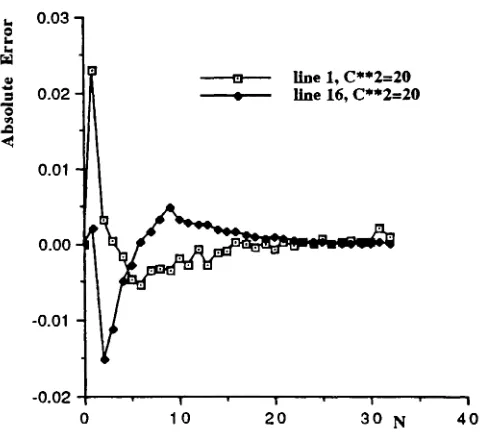
9, 10, · · · ,16. In figure 6, we plot the approximate and simulation results for the queue-length distribution of the cell processor queues corresponding to input line 1 ( the most heavily used) and input line 16 ( the least used). The value ofC2 was set to 20. The absolute errors are given in figure 6. The log(base 10) of the approximate and simulation results for the blocking probability for the same two cell processor queues are given in figure 6 as a function of

0

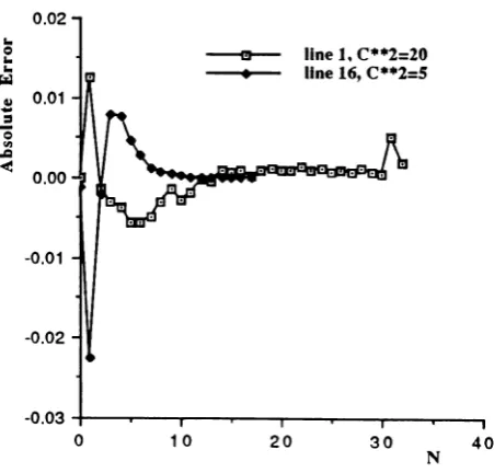
2

• The corresponding absolute errors are given in figure 6. Finally, figures 6 and 6 give results for the asymmetric case 2, assuming 02 = 20 for line 1 and C2

==

_{5 for line 16.}

From the above results, we see that the approximation algorithm has a satisfactory accuracy. The absolute error of the blocking probabilities becomes large when the average utilization of the input line is small or the squared coefficient of variation C2of the interarrival time is small. The reason for this is that we have observed empirically that the variance of the number of busy input lines depends on C2

• It becomes bigger when C2 is small, and

smaller when C2 _{is large. However, the way we calculate the probability of success,} _{1 -} _(J",

(17)

0.8

0.6

•

a

•

approx, , C··2=10 simulation ,C··2=10 approx., C··2=10000 simulation,C··2=10000

0.4

0.2

N 40

30 20

10

J.-...:.::~

..._ ....

~.---.

0.0

o

Figure 4: Queue length distribution for various values of C**2 (symmetric case).

0.02

..

Q

..

...

~

0.01

~

...

=

Q

(I)

..,Q

-e _0.00

-0.01

-0.02

•

C**2=lO C**2=lOOOO

40

N

30 20

1 0

-0.03 ..,....-..,....--r--..,...-..,...-~-..,...--..---..

o

(18)

0

~

'-"

OG

e

~

-1

~ approximation

•

simulation

-2

-3-+-~""""'~~---r'"""I'"""T"TT?onr----r''''''''''''''''''''''''---'-''''''''''~_

1 0 1

C**2

Figure 6: Approximation and simulation results for the blocking probability( symmetric case).

0.4

..

₀

..

~

~ _0.3

-; -0

(I)

-=

-e

0.2

0.1

0.0. J - _...-....,....,....,..,.,.,.,.n--..,.-.~~~..,...,I""'T'TTft"I'I

1 0 1

(19)

0.3

40

N 30

~ simulation, line 16

• approx., line 16

a simulation, line 1

o approx., line 1

20 10

0.0-L--,,....--~!II.,..:IJ

. . .

-.l.-,.-....,

o

0.1 0.2

Figure 8: Queue length distribution (asymmetric case 1, C**2:=20).

... 0.03

=

...

~

QI I!I line 1, C·*2=20

..

=

_0.02

•

_Une_{16, C**2=20}

e_~

.J:l

<

0.01 0.00 -0.01

40 30 N

20 10

-0.02- + - - - r - -...

---r----...----....----o

(20)

I!I simulation" One1

• approxbnation,Hoe1 a simulation,Hoe 16

• approxbnadon.llne16

0

::i ~

-1

"-'

0.0

C)

~

-2

-3

-4

-5

-6

0 100 200

C**2 300

Figure 10: Approximation and simulation results for the blocking probability (asymmetric case 1).

..

1.2

Q

....

~

~ 1.0

-;

-0_rn

0.8

.c

-e

0.6 0.4 0.2 -0.0 -0.2

0 100

~ line1

• line16

300

(21)

0.5

~

0.4

0.3

~ simulation. line 1

• approximation, line 1

a simulation, line 16

o approximation, line 16 0.2

40

N

30 20

10 0.1

0.0L~B.."""~=-~"

...

--""~--.,

o

Figure 12: Queue length distribution (asymmetric case 2).

0.02

..

e

..

~

~ 0.01

....

=

"0U')

.Q

~

0.00

-0.01

-0.02

-0.03

0 10 20

line 1. C··2=20 line 16, C·.2=5

30

N 40

(22)

7

Conclusion

A synchronous N x N Clos ATM switch with queueing capability at the input ports was

analyzed. The arrival process is modeled by an Interrupted Bernoulli Process. The proba-bility of success for transmission through the Clos switch was obtained approximately under an independent assumption and assuming that arrivals are Bernoulli distributed. The cell

processor queue was analyzed as an I B P/Geo

/1

queue first with infinite capacities and then

with finite capacities. Using the above results the ATM switch was then analyzed approx-imately. The approximation algorithm was extensively validated using simulation results. The algorithm has a satisfactory accurracy. The absolute error of the blocking probability increases when the average utilization of the input line is small or the squared coefficient of

variation 0 2 of the interarrival time is small.

References

[1]

Y. Oie, T. Suda, M. Masayuki, and H. Miyahara "Survey of the performance of

non-blocking switches with FIFO input buffers", IEEE International Conference on

Commu-nications VOL. 2, 737-741, 1990.

[2]

S.Z. Shaikh, M. Schwartz, and T.H. Szymanski "Analysis, control and design of crossbar

and banyan based broadband packet switches-for integrated traffic", IEEE International

Conference on Communications YOLo 2, 761-765, 1990.

[3] M.G. Hluchyj and M.J. Karol "Queueing in high-performance packet switching", IEEE

Journal on Selected Areas in Communications YOLo 6, NO.9, 1587-1597,1988.

[4] H. Yoon, K. Lee, and M. Liu "Performance analysis of multibuffered packet-switching

networks in multiprocessor systems", IEEE Transactions on Computers, VOL. 39, NO.

3, 319-327,1990.

[5] A.Huang and S. Knauer "Starlite: a wideband digital switch", IEEE GLOBECOM '84

Conf. Rec., 121-125, Nov. 1984.

[6] M. Devault, J.Y. Cochennec, and M. Serve! "The 'Prelude' ATD experiment: assess-ments and future projects", IEEE Journal on Selected Areas in Communications YOLo

6, NO.9, 1528-1537,1988.

[7] Janak H. Patel "Performance of Processor-Memory Interconnections for Multiproces-sors", IEEE Transactions on Computers, YOLo C-30, NO. 10, October 1981.

(23)

[9] Jeffrey J. Hunter "lvlathematical Techniques of Applied Probability :Discrete Time

Mod-els ", YOLo 2,1983

[10] M. F. Neuts "The single server queue ~n discrete time-numerical analysis, I", Naval Res. Logist. Quart. 20, 297-304, 1973.

[11] M. F. Klimko, and M. F. Neuts "The single server queue ~n discrete time-numerical analysis, If', Naval Res. Legist. Quart. 20, 304-319, 1973.

[12] M. F. Neuts, and M. F. Klimko "The single server queue in discrete time-numerical

analysis, IIf', Naval Res. Logist. Quart. 20,557-567, 1973.

[13] D. Heimann, and M. F. Neuts "The single server queue ui discrete time-numerical

analysis, I~'" , Naval Res. Logist. Quart. 20, 753-766, 1973.

[14]

Harry Heffes, and David M. Lucantoni "A Markov Modulated Characterization of