An Enriched Shell Finite Element for Progressive Damage Simulation in Composite Laminates.

(1)

ABSTRACT

MCELROY JR., MARK WAYNE. An Enriched Shell Finite Element for Progressive Damage Simulation in Composite Laminates. (Under the direction of Dr. Mark Pankow.)

A new formulation is presented for an enriched shell finite element capable of progressive damage simulation in composite laminates referred to as the Adaptive Fidelity Shell element.

The element enrichment is based on a combination of the Floating Node Method to enable

discrete representation of damage and a novel damage algorithm featuring the Virtual Crack Closure Technique. The element enrichment enables an adaptive mesh fidelity type approach

where an initial single layer of shell elements increases in fidelity locally as needed to suit

an evolving progressive damage process composed of multiple delaminations and transverse matrix cracks. Compared to alternative existing simulation techniques, use of the Adaptive

Fidelity Shell is more computationally efficient and demands less time and expertise from the

user. The Adaptive Fidelity Shell element was verified for a number of delamination problems using numerical benchmark data. These include Mode I, Mode II, mixed-mode, and multiple

crack problems. Initial experimental validation was performed using a previous

delamination-migration experiment. After the initial verification and validation, a new test method was developed where specimens were loaded using both quasi-static and dynamic loads to generate

damage processes slightly more complex than those of the initial delamination and

delamination-migration studies. The test had a dual purpose of (1) investigating in detail some of the damage mechanisms that occur during low-velocity impact and (2) using the experimental data for

model validation. The Adaptive Fidelity Shell model was used to simulate the quasi-static and

dynamic tests and in doing so provide some validation as well as highlighting areas that need improvement. Finally, the Adaptive Fidelity Shell was used in a blind prediction to simulate a

realistic low-velocity impact test. The blind prediction was partially successful although some

(2)

(3)

An Enriched Shell Finite Element for Progressive Damage Simulation in Composite Laminates

by

Mark Wayne McElroy Jr.

A dissertation submitted to the Graduate Faculty of North Carolina State University

in partial fulfillment of the requirements for the Degree of

Doctor of Philosophy

Aerospace Engineering

Raleigh, North Carolina

2016

APPROVED BY:

Dr. Kara Peters Dr. Jeff Eischen

Dr. Melissa Pasquinelli Dr. T. Kevin O’Brien

Dr. John Wang Dr. Mark Pankow

(4)

BIOGRAPHY

Mark (Mack) McElroy was born in Wilmington, Delaware (USA) in 1983. Growing up in rural Vermont, Mack formed an interest in science and engineering, and eventually enrolled at Lehigh

University in 2001 where he obtained a B.S. and M.S. in Civil Engineering. After a brief internship at a Civil Engineering firm, Mack used his focus in structures and mechanics to

obtain a job at Northrop Grumman Shipbuilding in Newport News, VA (now

Huntington-Ingalls Industries). There, he participated in the design of the new Ford class aircraft carrier for the U.S. Navy. When the ship design was complete, Mack left the shipyard and started

work at Pratt and Whitney in Hartford, CT where he focused on rotor dynamics simulation in

gas turbine engines. Mack’s early career experience led him to realize that he was interested in extending his education and as such returned to school for a PhD in Aerospace Engineering in

2012. Mack currently works at NASA Langley Research Center in Hampton, VA and likes to

(5)

ACKNOWLEDGEMENTS

There are many people to thank that assisted me with this body of work. Dr. Kevin O’Brien for giving me a chance, acting as a technical mentor, and undertaking a role of significance and

generosity in my life unmatched by anyone else outside of my family. My advisor, Dr. Mark Pankow, for helping me when I needed it the most, keeping me on track, and the technical

insight. Wade Jackson for working everyday with me on my tests. Sean Britton, Will Johnston,

and Peter Hellstrom for assisting with the tests. Spyros Tsampas for all of the SEM work. Dr. Erik Saether for getting into the details and helping with my code and element formulation. John

Wang for getting me going in the beginning and always there for consultation. Dr. Ron Kruger,

Dr. Frank Leone, Dr. Drew Bergan, Dr. Michael Czabaj, Dr. Cheryl Rose, and Dr. Carlos Davila for always willing to talk though technical issues. Dr. Gretchen Murri for teaching me how to

write a good paper. Donato Girolamo and Patrick Lesser for being there to share our common

struggles. Dr. Robin Olsson and Dr. Renaud Gutkin for the collaboration and technical input. Jonathan Ransom for hiring me into an extraordinary research and educational opportunity

and always willing to offer advice and support as needed. Dr. James Ratcliffe for being there

for me in the hardest of times. My family for the constant and unrelenting moral support. And Dr. Nelson De Carvalho for inspiring my research and teaching me daily about the secrets of

(6)

BIBLIOGRAPHY . . . .149

APPENDICES . . . .160

Appendix A Enriched Beam Element . . . 161

A.1 Element formulation . . . 161

A.2 Verification . . . 168

Appendix B Parametric Studies . . . 170

B.1 Solution increment size . . . 170

B.2 Critical migration angle, αc . . . 172

B.3 fIIc. . . 175

B.4 µ . . . 176

B.5 Gaussian smoothing . . . 177

(8)

LIST OF TABLES

Table 2.1 Required input parameters for enriched shell model . . . 42 Table 2.2 Numerical benchmark material and strength properties (all unidirectional

graphite/epoxy prepreg) [84]. . . 44 Table 2.3 Summary of mesh sizes considered in verification models (units in mm,

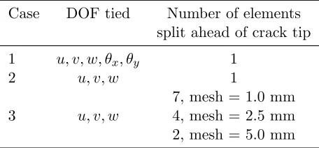
∆a/h0 corresponds to a subregion in a damaged element). . . 45 Table 2.4 Summary of three DCB cases with varying delamination front tied DOF

and number of elements split but tied ahead of the delamination. . . 46 Table 2.5 Delamination-migration: Migration location correlation summary. . . 72

Table 4.1 Material and strength properties for IM7/8552 [129]. . . 103 Table 4.2 Summary of parametric studies used to understand the ideal model

config-uration (each parametric study was perform using Layup 1 unless otherwise specified). . . 122

Table 5.1 Material and strength properties used in the blind prediction [132, 134]. . . 125 Table 5.2 Comparison of computational efficiency between AFS and HF-1 models. . 142

(9)

LIST OF FIGURES

Figure 1.1 Example of barely visible impact damage [10] . . . 2

Figure 1.2 Example of typical impact damage as observed by Choi et al. [14] with sequence of events identified by number. . . 3

Figure 2.1 Shell element schematic. . . 12

Figure 2.2 Laminate schematic (k = ply number,n = total number of plies, and β = ply orientation). . . 17

Figure 2.3 Element in natural coordinates. . . 20

Figure 2.4 Floating Node Method. . . 28

Figure 2.5 Virtual Crack Closure Technique tie forces and nodal displacements. . . . 30

Figure 2.6 Element splitting in the vicinity of a delamination front. . . 31

Figure 2.7 Delamination migration in a test specimen and in a solid element mesh. . 32

Figure 2.8 Representation of delamination migration in a shell mesh. . . 33

Figure 2.9 Delamination-migration prediction. . . 34

Figure 2.10 Delamination-migration prediction (3-D). . . 36

Figure 2.11 DCB specimen and model description. . . 45

Figure 2.12 Diagram of mesh for case 3: rotations are unconstrained in split element ties and multiple elements ahead of the delamination are split and tied together. . . 47

Figure 2.13 DCB: Force-displacement correlation. . . 48

Figure 2.14 Effect of constrained DOF at crack tip on VCCT forces and displacements for case 1 and case 2. . . 49

Figure 2.15 DCB: Tie forces in split elements ahead of crack tip andGI as a function of distance elements are split ahead of the delamination. . . 51

Figure 2.16 DCB: Results from mesh convergence study for normalized energy release rate, GT/GIc, distribution across delamination front (a =ao = 30.5 mm). 52 Figure 2.17 DCB: Delamination front geometry and energy release rate at the first instance of crack growth (a=ao = 30.5 mm). . . 53

Figure 2.18 Diagram of DCB specimen with a skewed crack front. . . 54

Figure 2.19 Diagram of (a) high-fidelity and (b) AFS finite element models of DCB skewed crack models. . . 55

Figure 2.20 Comparison of results from the high-fidelity and AFS models of the DCB skewed delamination specimen. . . 56

Figure 2.21 ENF specimen and model description. . . 57

Figure 2.22 ENF: Force-displacement data comparing nodal tie and surface based contact simulation techniques. . . 58

Figure 2.23 ENF: Force-displacement data correlation. . . 59

Figure 2.24 ENF: Results from mesh convergence study for normalized energy release rate, GT/GIIc, distribution across delamination front (a=ao = 25.4 mm). 60 Figure 2.25 MMB specimen and model description. . . 60

Figure 2.26 MMB: Force-displacement data correlation,GII/GT = 0.8. . . 61

(10)

Figure 2.28 SLB: Force-displacement data correlation,GII/GT = 0.4. . . 63

Figure 2.29 Summary of verification model runtimes . . . 64

Figure 2.30 Diagram of multiple crack DCB specimen . . . 65

Figure 2.31 Stiffness matrix for multiple delaminations . . . 66

Figure 2.32 Deformed plot of the multi crack DCB test modeled with the enriched shell elements . . . 66

Figure 2.33 Multi crack DCB: force-displacement correlation . . . 67

Figure 2.34 Delamination-migration test summary [49]. . . 68

Figure 2.35 Delamination-migration: Enriched shell finite element model of delamination-migration test (Figures from [49]). . . 69

Figure 2.36 Delamination-migration: Force-displacement correlation (error compared to average of experimental curves). . . 70

Figure 2.37 Delamination-migration: Migration location correlation. . . 71

Figure 3.1 Example of typical low-velocity impact damage in a laminate . . . 74

Figure 3.2 Test overview. . . 76

Figure 3.3 Test specimen description. . . 77

Figure 3.4 Quasi-static test setup. . . 78

Figure 3.5 Impact test details. . . 79

Figure 3.6 Multiple load cycles and summary force-displacement curve. . . 81

Figure 3.7 Layup 1 test results. . . 82

Figure 3.8 Delamination growth and migration detail (CT images from specimen XP3-6). . . 84

Figure 3.9 CT images of transverse matrix cracks forming incrementally before de-lamination growth initiation (specimen XP3-6). . . 85

Figure 3.11 CT scans showing “staggered migration” in Layup 2. . . 87

Figure 3.13 Delamination area versus specimen deflection for all quasi-static tests. . . 90

Figure 3.14 Low-velocity impact force-displacement data. . . 91

Figure 3.15 Representative UT scans of damage in impact and quasi-static tests. . . . 92

Figure 3.16 Energy required for initiation of delamination in the quasi-static and im-pact tests. . . 93

Figure 3.17 Investigation on error in force-displacement data from impact tests. . . 94

Figure 3.18 Measured forces from hammer and impact test load cells for centered and off centered load conditions (data points are summarized using a solid linear trendline to aid in comparison with the dashed line). . . 95

Figure 3.19 Example of before and after data plots using “back-calculated” deflection data from measured and corrected force. . . 97

Figure 3.20 Correlation of corrected impact data and quasi-static data. . . 98

Figure 3.21 SEM images showing cusp orientation. . . 99

Figure 3.22 SEM images showing transverse matrix crack face. . . 100

(11)

Figure 4.2 Force-displacement correlation between tests and the AFS model (Layup

1). . . 105

Figure 4.3 Qualitative correlation of delamination size and damage pattern (Layup 1).106 Figure 4.4 Quantitative correlation of delamination size (Layup 1). . . 107

Figure 4.5 Force-displacement correlation between tests and the AFS model (Layup 2). . . 107

Figure 4.6 Qualitative correlation of delamination size and damage pattern (Layup 2).108 Figure 4.7 Force-displacement correlation between tests and the AFS model (Layup 3). . . 109

Figure 4.8 Qualitative correlation of delamination size and damage pattern (Layup 3).110 Figure 4.9 Correlation of corrected impact test data and AFS model dynamic simu-lation (Layup 1). . . 112

Figure 4.10 Qualitative correlation of delamination size and damage pattern between tests and simulations for dynamic and quasi-static loads (Layup 1). . . 114

Figure 4.11 Correlation of corrected impact test data and AFS model dynamic simu-lation (Layup 2). . . 115

Figure 4.13 Correlation of corrected impact test data and AFS model dynamic simu-lation (Layup 3). . . 118

Figure 5.1 Example of the test fixture used in ASTM 7136. . . 124

Figure 5.2 3D impact model overview. . . 127

Figure 5.3 AFS impact model overview. . . 128

Figure 5.4 First ply failure prediction and seeded AFS delamination. . . 130

Figure 5.5 Delamination prediction correlation between test and AFS model. . . 131

Figure 5.6 Force and deflection correlations between test and AFS model. . . 134

Figure 5.7 Force and deflection correlations between test and calibrated AFS model. 136 Figure 5.8 Comparison of damage in un-calibrated AFS, stiffness calibrated AFS, and the test. . . 137

Figure 5.9 High fidelity model used in multiple delamination study. . . 138

Figure 5.10 Damage configuration and cohesive zone definitions in Models HF-1 and HF-2. . . 138

Figure 5.11 Force and deflection results in multiple delamination study. . . 140

Figure 5.12 Delamination pattern comparison in multiple delamination study. . . 141

Figure 5.13 Force-time and force-deflection comparison for different delamination seed geometries. . . 143

Figure 5.14 Delamination patterns predicted by various seed delamination geometries. 144 Figure A.1 Stiffness matrix for an exact Timoshenko beam element [85] . . . 162

(12)

Figure A.3 Stiffness matrix for an exact Timoshenko beam element offset by a

dis-tance d, including floating nodes . . . 164

Figure A.4 Stiffness matrix for an exact Timoshenko beam element split into two subregions each offset by a distance d . . . 165

Figure A.5 Stiffness matrix for an exact Timoshenko beam element split into two subregions each offset by a distance d. Nodal ties are applied at one end of the element (ktie is a large stiffness term approximately 1000 times greater than K₁₁(e)). . . 166

Figure A.6 VCCT schematic for enriched beam element . . . 167

Figure A.7 Beam DCB: Force-displacement data correlation . . . 168

Figure A.8 Beam ENF: Force-displacement data correlation . . . 169

Figure A.9 Beam MMB: Force-displacement data correlation,GII/GT = 0.8 . . . 169

Figure B.1 Parametric study on solution increment size (the condition used in all other simulations is outlined). . . 172

Figure B.2 Parametric study on critical migration angle for Layup 1 (the condition used in all other simulations is outlined). . . 173

Figure B.5 Parametric study on Mode II critical energy release rate increase factor at the insert boundary (the condition used in all other simulations is outlined).176 Figure B.6 Parametric study on the coefficient of friction between Mode II crack surfaces in Layup 1 (the condition used in all other simulations is outlined).177 Figure B.7 Parametric study on the coefficient of friction between Mode II crack surfaces in Layup 3 (the condition used in all other simulations is outlined).178 Figure B.8 Example of smoothing energy release rate and delamination growth di-rection on nodes across a delamination front at an arbitrary damage state in Layup 3. . . 179

Figure B.9 Parametric study on the influence of smoothingG(mig)andθon a delam-ination front in Layup 3 (the condition used in all other simulations is outlined). . . 179

Figure B.10 Parametric study on the influence of smoothing GT on a delamination front in Layup 1 (the condition used in all other simulations is outlined). 180 Figure B.11 Summary of two techniques to calculateG(mig). . . 181

Figure B.12 Parametric study comparing two techniques for calculating G(mig) in Layup 1 (the condition used in all other simulations is outlined). . . 182

(13)

Chapter 1

INTRODUCTION

The use of lightweight composite materials in new aircraft designs is one means of increasing

energy efficiency and decreasing operating costs compared to legacy aircraft constructed from

traditional materials such as aluminum. A challenge with using composite materials is their susceptibility to brittle failure resulting from transverse loads such as impact [1].

Addition-ally, because residual strength after impact can be lower than the original strength, in-plane

compressive loading after impact may result in further damage growth and eventual structural failure even if the initial impact damage was minimal [2–4]. Therefore, for composite structures

to be reliable and safe they must be designed and certified to survive some level of impact

damage and subsequent compressive loading.

Certification of structural components is performed by testing or simulation. The latter is

usually preferred, if it is possible, due to the lower relative cost. Currently, a lack of reliable and

robust simulation tools for progressive damage in composite laminates results in a high reliance on testing for certification [5–7]. Reliable and cost effective simulation of progressive damage

occurring during or after impact damage could potentially reduce the need for testing [8, 9].

Additionally, an efficient tool of this nature may allow for better component design early on and prevent costly redesigns.

Some typical causes of impact loads are hail, bird strike, tool drops, or baggage cart

colli-sions. Tool drops and baggage cart collisions fall into the category of low-velocity impact which can be particularly concerning because damage is often not visible externally, but can be

signifi-cant in the interior of a laminate. This is commonly referred to as barely visible impact damage (BVID). An example of BVID is shown in a cross section of a laminate in Figure 1.1 [10].

Here, the damage is not visible externally, but internally is extensive and consists of multiple

(14)

tool applicable to low-velocity impact or compression after impact (CAI) must be capable of capturing the physics within a progressive damage process that results in this type of damage

pattern.

Matrix crack Delamination

Figure 1.1 Example of barely visible impact damage [10]

1.1

Background

A prerequisite for using composite materials in aerospace structures is an understanding of

damage resulting from low-velocity impact and what this means in terms of the structure’s performance and safety. Study of impact loading and damage prediction in composite laminates

dates back to the 1970s [11]. Much of the early work in this field was experimental and directed towards observing the nature of damage that forms during low-velocity impact [12–14]. Of

particular note is the study by Choi et al. where impact testing was performed on cross-ply

specimens in order to render the physical response effectively into two dimensions (2D). In doing this, the failure mechanisms could be better observed and understood. Choi et al.’s work

showed the fundamental process that occurs in a low-velocity impact, illustrated in Figure 1.2,

where (1) matrix cracks first form, either in the tensile region due to bending, or elsewhere due to transverse shear (depending on layup) and (2) matrix cracks grow out-of-plane until a ply

interface of dissimilar fiber orientation is reached where delamination can initiate.

Other research in this time frame dealt with development of analytical predictive tools, including prediction of impact force response [15–18]. In some cases, analytical tools included not

only impact force response, but also a means to predict the onset and extent of damage [19–23].

Analytical models such as this are useful in certain design applications; however, they have limited ability to address problems that involve complex damage processes consisting of many

(15)

0°

90°

0°

(b)

transverse

shear

cracks

0°

90°

(a)

tension

cracks

90°

=

matrix

crack

=

delamination

impact

load

impact

load

1

2

1

2

Figure 1.2 Example of typical impact damage as observed by Choi et al. [14] with sequence of events identified by number.

boundary conditions. One means to address these types of complexities is through the use of

finite element models.

Finite element (FE) simulation of progressive damage in laminates from low-velocity impact began in the 1990s [24–26]. Since then, progressive damage simulation in laminates has advanced

considerably due partially to advances in computational technology, but also due to advances

in numerical simulation techniques. Two fracture based techniques, cohesive zone (CZ) and the Virtual Crack Closure Technique (VCCT), are used commonly for crack growth simulation

in FE models. CZ modeling was initially used to simulate crack growth in metals [27]. An

initial cohesive FE formulation was presented by Beer in 1985 [28], and has since seen many enhancements for use in laminate damage simulations, including accommodation of mode-mixity

[29, 30]. An alternative technique to CZ modeling is VCCT [31]. First presented by Rybicki

[32, 33], VCCT was first used in the context of damage prediction in laminates as early as the late 1970s and 1980s [34, 35].

CZ modeling and VCCT each have advantages and disadvantages. CZ models have solution convergence difficulties and also generally require a very fine mesh [36]. On the other hand,

initiation and growth are both inherently built into the technique, which is not the case with

(16)

CZ models are largely avoided in VCCT. Both CZ and VCCT are used for laminate damage simulation in current state-of-the-art damage models [37].

Simulating a progressive damage process of the types seen in Figures 1.1 and 1.2, requires the

consideration of interacting transverse matrix cracks and delaminations. Finite element models aimed at capturing this type of behavior in detail became possible only when numerical and

computational tools became sufficiently robust [37]. Many FE models began to combine several

damage simulation techniques into the same model. Continuum damage mechanics (CDM) [38–40], based on degradation of element material properties in an area of damage, and the

eXtended Finite Element Method (XFEM) [41, 42], based on a discrete discontinuity in a mesh

displacement field, have emerged as two approaches used in FE modeling in conjunction with CZ and VCCT techniques.

Many state-of-the-art simulation models for progressive damage in laminates are

combina-tions and variacombina-tions of the techniques mentioned above. Additionally, most models fall into one of two categories where intralaminar damage such as fiber failure and matrix cracking are

simulated with CDM [43–45] or where the intralaminar damage is simulated discretely [46–48]. The use of CZ approach for delamination failure is common in both of these methods, although

VCCT has also been used [49, 50]. The two approaches have also been combined such that fiber

failure is simulated with CDM, and intralaminar matrix cracks and delamination are modeled discretely [51, 52].

FE models that use combinations of CDM, XFEM, VCCT, and CZs for progressive damage

simulation tend to be high-fidelity in nature, consisting of a level of mesh discretization of at least one element per ply. Model fidelity is typically high for two main reasons. First, a

fine mesh with at least one element per ply allows for detailed stress and strain through the

laminate thickness in each ply to be calculated and used in a criterion to predict initiation and propagation of damage. Second, representation of a three-dimensional damage pattern, as

dictated by the prediction, is intuitive in a mesh that is also three-dimensional. A disadvantage of

high-fidelity meshes, in general, is that they are very inefficient, as a large amount of information is determined throughout the entire model when this level of detail is only needed at locations

where a damage process is occurring.

Laminates used in structures can have dozens of plies or more, so use of models that rely on a discretization level of at least one element per ply in the thickness direction is limited not

only by their computational demand, but also by the complexity of the process required by the

user to create and verify a model. Current numerical damage simulation techniques using finite elements have yet to be demonstrated to be accurate in a consistent and general manner for

(17)

(i.e., simple relative to a realistic scenario where a laminate may have dozens of plies with damage propagating three-dimensionally throughout the entire layup) [37, 53]. Hence, more

efficient models and simulation techniques that demand less computationally, as well as require

less time and expertise from the user, are desirable.

1.2

Damage simulation with shells

Use of shell element models may offer an alternative to existing high-fidelity methods. Shell elements have long been used by industry and have proven to be a cost effective analysis

tool, albeit, for problems less complex than laminate damage simulation. Shell element models

are computationally efficient and generally require less training and time for an analyst to use when compared to a high-fidelity solid element model. Use of shell element models for

laminate damage simulation, however, introduces a number of challenges, including prediction

and representation of transverse matrix cracks and delaminations at multiple interfaces. Previous use of shell elements for progressive damage simulation has consisted of either a

global-local approach [54], where the actual damage simulation takes place in a high-fidelity

region attached to an otherwise low-fidelity model, or by stacking layers of shell elements to form a laminate [55–59]. In the stacked shell approach, independent layers of shell elements

are defined and connected across ply interfaces in a laminate. If delamination at a specific ply

interface is of interest, a mesh may consist of two layers of shell elements, one on either side of the ply interface location. The two layers can be connected by a CZ or by rigid links and

delamination growth is predicted with a cohesive law or VCCT, respectively.

Wang et al. [60, 61] studied the use of VCCT for delamination prediction between stacked shell elements. This work (along with a related study [62]) indicate that mixed-mode energy

re-lease rate can be calculated using shell elements; however, continued mesh refinement may

not result in converged values in some cases. Similarly, in bimaterial crack tip interfaces, energy release rate component divergence is observed with mesh refinement near the crack

tip/delamination front when using VCCT with any element type. Previous work indicated that

this non-convergence may be avoided by establishing a minimum mesh size based on the ratio of incremental crack growth length in the mesh to element thickness, ∆a/h [63].

An inherent disadvantage of the two-layer stacked shell models is that the delamination interface in a laminate must be predefined, thereby limiting the model’s utility as a general

predictive tool. Furthermore, by restricting the delamination to a single ply interface location,

(18)

layer of shells for every ply and stacking all of the layers to form the laminate. This type of approach; however, begins to share some of the same drawbacks mentioned for high-fidelity

solid element models, namely lengthy and complex model preparation and high computational

demand.

Ideally, in terms of computational efficiency; ease of use; and predictive utility, a thin

lam-inate plate would be modeled as a single layer of shell elements in which delaminations could

form and propagate at any location in the layup. This type of approach can be thought of as having adaptive fidelity in that the model is defined initially in low-fidelity (one shell

ele-ment thick) and remains in this state everywhere except locally where delamination occurs and

multiple layers are required as dictated by a damage prediction criteria throughout an anal-ysis solution procedure. Effectively, in the local damaged regions, the stacked shell technique

described previously is used.

Simulation models based on shell elements that use adaptive fidelity have been proposed and studied only recently. Larsson presented a shell element in 2004 [64] that treats delaminations

as an in-plane discontinuity in the displacement field in a shell formulation and uses a cohesive zone to predict growth. Similarly, Brouzoulis et al. [65–67] have developed a shell element that

uses XFEM and cohesive zones to simulate growth of multiple delaminations and transverse

matrix cracks in a shell element. Their work is ongoing but, while showing promise, has not yet advanced to the point of being able to simulate a realistic and practical progressive damage

problem such as low-velocity impact.

Since the development of XFEM, several variations and improvements have been proposed, including Regularized-XFEM [68] and the Phantom Node Method [69]. A more recent study was

published on the newly introduced Floating Node Method (FNM) [70]. The FNM’s technique

for numerical discrete damage representation has an inherent simplicity, compared to the other techniques mentioned, that makes it straightforward to implement and easy to modify and

customize. Additionally, it offers some advantages related to element crack mapping and the

integration procedure [70].

When using the FNM to introduce mesh discontinuities representative of damage growth, a

crack propagation technique is needed. VCCT offers an efficient numerical solution procedure

and largely avoids convergence difficulties and mesh refinement requirements that are associ-ated with the use of cohesive zones. Studies have shown that when using a transverse shear

deformable shell element, mixed-mode energy release rates can be calculated accurately with

VCCT [50,59,62,71,72]. Furthermore, it was shown that VCCT could be successfully combined with the FNM to model crack growth [49], though this was not using shell elements.

(19)

is not aligned with the mesh. Though this difficulty has been studied and solutions have been proposed that can generate accurate behavior [73–76], it remains an additional challenge for

any numerical implementation.

The ability to predict transverse cracks that form adjacent to or along side of delami-nations in shell models has received little attention in the past as it is seemingly unnatural

to consider out-of-plane damage features in planar elements. This damage mechanism has

been described as “delamination-migration” [77]. Studies have shown that the occurrence of delamination-migration in a crossply specimen can be described as a function of the sign of

the in-plane shear force at the delaminated interface between the “upper” and “lower” groups

of intact plies around a delamination crack front [77, 78]. Additionally, similar work suggests that delamination-migration may be able to be predicted using energy release rates associated

with orthogonal shear delamination growth directions at a given location [79–82]. Drawing from

conclusions reached in this selection of work, shear energy release rates determined using VCCT forces at tied delamination front nodes, and the shear force sign between “upper” and “lower”

regions of a delamination front may be used to determine the preferential growth direction in three-dimensional space of the delamination.

1.3

Problem statement

The goal of this dissertation is to present the formulation, verification, and validation of a novel enriched shell finite element capable of progressive damage simulation in composite laminates.

The capability to predict mixed-mode delaminations, delamination-migration, and low-velocity

impact damage is included. The intent is that this new simulation approach will be signif-icantly more efficient and cost effective than existing tools and therefore enable progressive

damage simulation in industry where it currently is cost prohibitive. The overall challenge

con-fronted in this work was creation of a methodology where, compared to legacy tools, model fidelity is reduced but prediction accuracy is maintained. Roles of the enriched shell model in

industrial application may include (1) rapid design tool, (2) simulate damage processes that are

currently too complex to simulate with available high-fidelity models, or (3) replace existing costly modeling tools. As part of the model formulation and development, the enriched shell is

used to identify and investigate limitations and future areas of research related to progressive damage simulation using shell elements.

The element enrichment allows for adaptive mesh fidelity in which a single element splits

(20)

and a single shell element is used to represent the entire laminate thickness as defined in the beginning of the analysis. This capability is achieved using the Floating Node Method to

dis-cretely represent a delamination in the mesh and VCCT to predict its growth. The element is

coded as a user-subroutine in Abaqus 6.14/Standard [83]. Details concerning the use of VCCT in conjunction with shell elements, mesh dependency of the solution, and out-of-plane damage

formation are investigated via analysis and testing.

1.3.1 Research questions

The following research questions will be discussed and answered in this dissertation:

1. How well can mixed-mode delamination be simulated using shell elements?

2. How can three-dimensional progressive damage processes involving delamination and transverse matrix cracks be represented and predicted in a shell element model?

3. What is the physical configuration of matrix cracks linking delaminations at different

interfaces in a low-velocity impact damage pattern?

4. What are the limitations of a shell element model for progressive damage simulation in

composites?

1.3.2 Unique contributions

The unique contributions to the scientific community found in this dissertation can summarized

as follows:

1. An approach for simulating progressive damage in composite laminates with novelty lying

in the following: (1) use of a shell element formulation, (2) implementation of the Virtual Crack Closure Technique, (3) implementation of the Floating Node Method, and (4) a

method to both predict and represent transverse damage features (i.e., such as matrix

cracks).

2. Deeper fundamental understanding of fracture patterns that occur during low-velocity impact in composite laminates.

3. A new test method and experimental data useful for model development and validation. Specifically, the test data is more complex than a standard delamination coupon but less

(21)

4. Identification and discussion on the limitations and future challenges in simulating 3D laminate progressive damage with shell elements.

1.3.3 Dissertation Outline 1. Introduction

2. Model Formulation

3. Biaxial-bending Tests: Experiments

4. Biaxial-bending Tests: Simulations

5. Low-velocity Impact Simulation

6. Conclusions

7. Bibliography

8. Appendix A: Enriched Beam Element

(22)

Chapter 2

Model Formulation

In this section, a finite element formulation is presented for an enriched shell element capable

of progressive damage simulation in laminates that is referred to as the Adaptive Fidelity Shell

(AFS) element. In addition to the formulation, verification and validation of the element are also presented. The following is intended to provide a reader knowledgeable in the finite element

method and fracture mechanics enough information so that they may recreate the model if

desired.

2.1

Beam element

As a first step, an enriched beam element was created to serve as proof of concept for the more advanced shell formulation. A shear deformable element was selected based on the

Tim-oshenko formulation. The beam is enriched with the Floating Node Method (FNM) in order

to represent delaminations and uses a damage algorithm based on the Virtual Crack Closure Technique (VCCT). The FNM enrichment and damage algorithm are directly analogous to

the shell formulation described in Section 2.2.2 and Section 2.2.3. To avoid redundancy and to

focus on the main goal of research (i.e., the shell element) further detail on the beam element formulation is omitted at this time, but included in summary in Appendix A. Also included in

Appendix A is verification of the enriched beam element using numerical benchmark data for

(23)

2.2

Shell element

The following is a description of the formulation of the Adaptive Fidelity Shell element. Much

of the element formulation presented here is based on information presented by Onate in [85] for a laminate Mindlin shell element. Using this formulation, and after addressing shear locking

and applying layerwise shear correction factors, the element is suitable for thick and thin (i.e.,

transverse shear or bending dominated) shells. The AFS element is enriched with the Floating Node Method and uses the Virtual Crack Closure Technique to perform discrete laminate

damage simulations. This section demonstrates how the element stiffness matrix, K(e), for the enriched shell, is obtained using the well known expression for a linear elastic element

K(e)=

Z

xyz

BTDBdV (2.1)

whereB is the strain-displacement matrix andD is the constitutive material matrix.

2.2.1 Mindlin shell

2.2.1.1 Baseline formulation

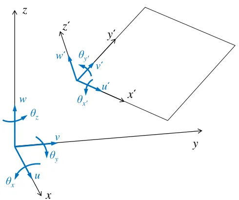
A four node shell element with five degrees-of-freedom (DOF) per node is shown in three-dimensional space in Figure 2.1. The node and DOF labels as defined in Figure 2.1 are used

henceforth. The prime superscript refers to a local (i.e., element) coordinate system which may

be oriented arbitrarily in global three-dimensional space. The element displacement field, in three orthogonal components, is described by

u0(x0, y0, z0) =u0_o(x0, y0)−z0θx(x0, y0) (2.2a) v0(x0, y0, z0) =v0_o(x0, y0)−z0θy(x0, y0) (2.2b) w0(x0, y0, z0) =w0_o(x0, y0) (2.2c)

(24)

z

x

y

w u v θx θy θ_z

x

̒

y

̒

z

̒

w ̒

u ̒ v ̒

θ_x′ θ_y′

Figure 2.1 Shell element schematic.

field is described by



 

u0(x0, y0, z0) v0(x0, y0, z0) w0(x0, y0, z0)





=Na

(e)

= 4

X

i=1

Niai =

h

N1 N2 N3 N4

i       a1 a2 a3 a4       (2.3)

wherei= node number,

ai =

       

u0_i v_i0 w0_i θ_xi0 θ0_yi

(25)

and

Ni=

       

Ni 0 0 0 0

0 Ni 0 0 0

0 0 Ni 0 0

0 0 0 Ni 0

0 0 0 0 Ni

        (2.5)

Standard linear shape functions are used and defined as

N1 = 1/4(1−x0)(1−y0) (2.6a)

N2 = 1/4(1 +x0)(1−y0) (2.6b)

N3 = 1/4(1 +x0)(1 +y0) (2.6c)

N4 = 1/4(1−x0)(1 +y0) (2.6d)

The element strain field, εεε, may be divided into a planar component and a transverse shear component,εεεp and εεεs, respectively. Assuming plane stress conditions (i.e., σ0z = 0) the strain field is defined as

ε εε=

" εεεp ε ε εs # =         εx εy γxy γxz γyz         =        

∂u0/∂x0 ∂v0/∂y0 ∂u0/∂y0+∂v0/∂x0 ∂u0/∂z0+∂w0/∂x0 ∂v0/∂z0+∂w0/∂y0

        =        

∂u0_o/∂x0 ∂v_o0/∂y0 ∂u0/∂y0+∂v0/∂x0

0 0         +        

−z0(∂θ0_x/∂x0) −z0(∂θ0_y/∂y0) −z0(∂θ_x0/∂y0+∂θ0_y/∂x0)

∂w0_o/∂x0−θ0_x ∂w0_o/∂y0−θ0_y

        (2.7)

(26)

deformation mode independently from the others. Generalized strain is related to strain by

ε ε

ε=Sεεε(g) (2.8)

where S=        

1 0 0 −z0 0 0 0 0

0 1 0 0 −z0 0 0 0

0 0 1 0 0 −z0 0 0

0 0 0 0 0 0 1 0

0 0 0 0 0 0 0 1

        (2.9)

andεεε(g) is given by

ε εε(g)=



 

ε εε(g)m ε εε(g)_b ε εε(g)s

  = 4 X i=1                

(∂Ni/∂x0)u0oi (∂Ni/∂y0)v0oi

(∂Ni/∂y0)u0oi+ (∂Ni/∂x0)v0oi (∂Ni/∂x0)θxi0

(∂Ni/∂y0)θyi0

(∂Ni/∂y0)θxi0 + (∂Ni/∂x0)θyi0 (∂Ni/∂x0)w0_oi−Niθ0_xi (∂Ni/∂y0)w0oi−Niθ0yi

                (2.10)

whereiis equal to node number.

A relation between the generalized strains, εεε(g)_{, and the nodal displacements,} _a

i, is estab-lished using the strain-displacement matrix, B, as

ε ε ε(g) =

4

X

i=1

Biai =

h

B1 B2 B3 B4

i       a1 a2 a3 a4       (2.11)

(27)

respec-tively) can be segregated and Bi can be expressed as

Bi=



 

B(m)_i B(b)_i B(s)_i





 (2.12)

where

B(m)_i =



 

(∂Ni/∂x0) 0 0 0 0

0 (∂Ni/∂y0) 0 0 0 (∂Ni/∂y0) (∂Ni/∂x0) 0 0 0





 (2.13)

B(b)_i =



 

0 0 0 (∂Ni/∂x0) 0 0 0 0 0 (∂Ni/∂y0) 0 0 0 (∂Ni/∂y0) (∂Ni/∂x0)





 (2.14)

B(s)_i =

"

0 0 (∂Ni/∂x0) −Ni 0 0 0 (∂Ni/∂y0) 0 −Ni

#

(2.15)

Classical laminate theory is used to determine the constitutive material matrix, D, for a composite section consisting of multiple orthogonal plies with varying fiber orientations. For a single ply with a fiber orientation,β, that is aligned with the x0-axis in the element coordinate system (i.e.,β=0◦), the constitutive in-plane and transverse shear material matrices, D(p) and D(s), respectively, are defined as

D(p)=



 

E1/(1−ν12ν21) E2ν12/(1−ν12ν21) 0 E2/(1−ν12ν21) 0

sym. G12





 (2.16)

and

D(s)=

"

G13 0

0 G23

#

(2.17)

(28)

in-plane normal-to-fiber, and out-of-in-plane normal-to-fiber directions, respectively. For plies where the fiber orientation,β, is non-zero, D(p) and D(s) should be rotated about the elementz0-axis using transformation matrices ¯T1 and ¯T2 to obtain the material matrix. The rotated ply level constitutive material matrices, ¯D(p) and ¯D(s), are determined by

¯

D(p) = ¯TT₁D(p)T¯1 (2.18a)

¯

D(s)= ¯TT₂D(s)T¯2 (2.18b)

where

¯ T1 =



 

cos2(β) sin2(β) cos(β)sin(β) sin2(β) cos2(β) −cos(β)sin(β) −2cos(β)sin(β) 2cos(β)sin(β) cos2(β)−sin2(β)





 (2.19)

and

¯ T2 =

"

cos(β) sin(β) −sin(β) cos(β)

#

(2.20)

The rotated shear matrix, ¯D(s), should be further modified by applying shear correction factors, c11 and c22. The shear correction factors, discussed in Section 2.2.1.2, are applied and a shear material matrix, ¯D(scf), that is both rotated and includes shear corrections is defined as

¯

D(scf) =

"

c11D¯(s)11 D¯ (s) 12 ¯

D(s)₂₁ c22D¯(s)22

#

(2.21)

(29)

using the following equations

D(m)= h/2

Z

−h/2 ¯

D(p)dz0 = n

X

k=1 tkD¯

(p)

k (2.22a)

D(mb)=− h/2

Z

−h/2

z0D¯(p)dz0 =− n

X

k=1 tkz¯kD¯

(p)

k (2.22b)

D(b)= h/2

Z

−h/2

z02D¯(p)dz0= n X k=1 1 3 h

z_k+13 −z3_kiD¯(p)_k (2.22c)

D(s)= h/2

Z

−h/2 ¯

D(scf)dz0= n

X

k=1

tkD¯(s)k (2.22d)

wherek is the ply number andzk,tk,h, and ¯zk are thickness measures of the layup as defined in Figure 2.2. The constitutive material matrix, D, for a laminate is given as

D=



 

D(m)₃_×₃ D(mb)₃_×₃ 0₃_×₂

D(mb)3×3

D(b)₃_×₃ 0₃_×₂

02×3

0₂_×₃ D(s)₂_×₂





 (2.23)

k= 1 k= 2 k= n

. . . -h/2 h/2 t₁ t₂ t_n

laminate neutral axis

𝑧 1 𝑧 2 𝑧 𝑛

ply 1 neutral axis ply 2 neutral axis ply nneutral axis

β1

β2

βn

h z2

z₁ z_n

𝑧′

(30)

2.2.1.2 Shear correction factors

Shear correction factors in equation 2.21, c11 and c22, are determined for each ply, k, using a method presented by Laitinen et al. [86]. Based on work by Vlachoutis [87], Laitinen et al.’s

method is applicable to a general laminate ofnplies with each having an arbitrary orientation,β. The method is based on determining the ratio of strain energy assuming transverse shear strain is constant and the strain energy assuming transverse shear strain has a parabolic distribution.

This technique assumes cylindrical bending and determines the shear correction factors as a

function of ply location in the layup and ply fiber angle. The shear correction factors for a ply are given by

cψψ = R2_ψ dψIψ

ψ= 1,2 (2.24)

whereψis the direction in the laminate plane (i.e., 1 or 2). Laitinen definesRψ,dψ, andIψ for a laminate containingn layers as

Rψ = 1 3 n X k=1 ¯ Q(k)_ψψ

h

(zk−z¯nψ)3−(zk−1−z¯nψ)3

i

(2.25)

dψ = n

X

k=1 ¯

Q(k)_δδ(zk−zk−1) δ =ψ+ 3 (2.26)

Iψ = n

X

k=1 zk

Z

zk−1

g2_ψ(z0) ¯ Q(k)_δδ

dz0 (2.27)

where

gψ(z0) =− 1 2

nk−1 X

k=1

¯

Q(k)_ψψh(zk−z¯nψ)2−(zk−1−z¯nψ)2

i

− (2.28)

1 2

¯ Q(k)_ψψ

h

(31)

and

¯ znψ =

1 2

Pn

k=1Q¯ (k)

ψψ zk2−zk2−1

¯

Q(k)_ψψ(zk−zk−1)

(2.29)

In equations 2.25-2.29,n= total number of plies,nk = the current ply, and ¯Qis defined for each ply, k, as

¯ Q=

"

¯

D(p) 0

0 D¯(scf)

#

(2.30)

2.2.1.3 Shear locking

Mindlin shell elements that have a slender aspect ratio are subject to shear locking. This

in-accuracy is the result of transverse shear terms dominating the stiffness matrix as the element

thickness goes to zero (i.e., a slender aspect ratio). In practice, this may result in overly stiff elements under bending dominated deformations. Onate et al. present a methodology to

over-come shear locking based on an assumed shear strain distribution that results in an element

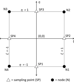
which is accurate in bending for thick and thin shells [88]. The following is a description of how to apply the methodology. For an element in its natural coordinate system, as shown in

Figure 2.3, the transverse shear strains are assumed to follow a linear distribution in the (ξ,η) coordinate system asγξ=α1+α2η and γη =α3+α4ξ. In matrix form, this can be expressed as " γξ γη # = "

1 η 0 0

0 0 1 ξ

#       α1 α2 α3 α4       (2.31)

The 2×4 coefficient matrix in equation 2.31 will be designated asA. Theαparameters can be determined by sampling tangential transverse shear strains at the edges of an element at

(32)

η

ξ η = 1

N4 N1

N2 N3

η = ‐1

ξ = 1 ξ = ‐ 1 SP1 SP2 SP3 SP4 = sampling point (SP) = node (N) (0,0)

Figure 2.3 Element in natural coordinates.

strain at the four sample points is given by

γ(1)=α1+α2η(1)=α1−α2 (2.32a) γ(2)=α3+α4ξ(2)=α3+α4 (2.32b) γ(3)=α1+α2η(3)=α1+α2 (2.32c) γ(4)=α3+α4ξ(4)=α3−α4 (2.32d)

or in matrix form as

      γ(1) γ(2) γ(3) γ(4)       =      

1 −1 0 0

0 0 1 1

1 1 0 0

0 0 1 −1

(33)

Designating the 4×4 coefficient matrix in equation 2.33 as P, the α values are determined by

α

αα=P−1γγγ (2.34)

The tangential transverse shear strains,γ(i), can be related to the shear strains,γξ and γη, by

      γ(1) γ(2) γ(3) γ(4)       =      

1 0 0 0 0 0 0 0

0 0 0 1 0 0 0 0

0 0 0 0 1 0 0 0

0 0 0 0 0 0 0 1

                     

γ_ξ(1) γη(1) γ_ξ(2) γη(2) γ_ξ(3) γη(3) γ_ξ(4) γη(4)

                (2.35)

If the 4×8 coefficient matrix in equation 2.35 is designated as T, then the transverse shear strain field can be described in terms of values at the sampling points as

" γξ γη

#

=AP−1T

               

(34)

Recall that, in element coordinates,γγγ =B(s)a(e), or in matrix form                

γxz(1) γyz(1) γxz(2) γyz(2) γxz(3) γyz(3) γxz(4) γyz(4)

                = h

B(s)₁ B(s)₂ B(s)₃ B(s)₄

i                             u1 v1 w1 θx1 θy1 . . . u4 v4 w4 θx4 θy4                             (2.37)

The relationship between shear strain in natural and element coordinates is based on the Ja-cobian matrix (discussed in Section 2.2.1.4) and in this case written as

               

                =      

[J]2×2 [0]2×2 [0]2×2 [0]2×2 [J]2×2 [0]2×2 [0]2×2 [J]2×2 [0]2×2

sym. [J]2×2

                     

γxz(1) γyz(1) γxz(2) γyz(2) γxz(3) γyz(3) γxz(4) γyz(4)

                (2.38)

(35)

on the assumed linear distribution can be defined as

" γxz γyz

#

=J−1

" γξ γη

#

=J−1AP−1TCB(s)

                            u1 v1 w1 θx1 θy1 . . . u4 v4 w4 θx4 θy4                             (2.39)

or, in a reduced form

γγγ = ¯B(s)a(e) (2.40)

where ¯B(s) represents the modified shear strain-displacement matrix to be used in the stiffness matrix calculation, and is given by

¯

B(s)=J−1AP−1TCB(s) (2.41)

2.2.1.4 Stiffness matrix integration

Full integration is performed using Gaussian quadrature in the natural element coordinate system. Natural coordinates are used as convenient integration bounds of -1 and 1. A

counter-clockwise node numbering convention is used as shown in Figure 2.3. The Jacobian matrix is

used to relate derivatives with respect to natural coordinates to those with respect to element coordinates. In defining the strain-displacement matrix, B, it is necessary to evaluate shape function derivatives with respect to element coordinates x0 and y0. In general these may be related to derivatives with respect toξ and η as

"

∂Ni/∂ξ ∂Ni/∂η

#

=J

"

∂Ni/∂x0 ∂Ni/∂y0

#

(36)

Thus, if integration is performed using the natural coordinate system, the shape functions are defined using node locations in the natural coordinate system, and the associated derivatives

with respect tox0andy0seen in equations 2.13-2.15 should be multiplied by the Jacobian inverse as

"

∂Ni/∂x0 ∂Ni/∂y0

#

=J−1

"

∂Ni/∂ξ ∂Ni/∂η

#

(2.43)

whereJ−1 is given by

J−1= 1 det(J)

"

J22 −J12 −J21 J11

#

(2.44)

For a four node planar element, such as a shell, the Jacobian matrix is defined as

J= 1 4

"

−(1−η) (1−η) (1 +η) −(1 +η) −(1−ξ) −(1 +ξ) (1 +ξ) (1−ξ)

#      

x1 y1 x2 y2 x3 y3 x4 y4

      (2.45)

where xi and yi are global nodal coordinates. The stiffness matrix is calculated as shown in equation 2.1, but in the natural coordinate system and with the modified strain-displacement

and material matrices derived in Sections 2.2.1.1-2.2.1.3 as

K(e)= 1 Z −1 1 Z −1 ¯

BTDB¯det(J)dξdη (2.46)

Or using Gaussian quadrature,

K(e)= 2 X i=1 2 X j=1 ¯

B(ξi, ηj)TDB¯(ξi, ηj)det(J)WiWj (2.47)

Using full integration, the weight terms,Wi andWj, can be set equal to 1.0 if the following locations in the natural coordinate system are used for the four integration points: 1/√3, 1/√3, -1/√3, 1/√3, -1/√3, -1/√3, and 1/√3, -1/√3.

Finally, once the element stiffness matrix has been obtained, it should be transformed into

(37)

rotated in three-dimensional space, can result in a third rotational component θz that is not present in the element formulation. The stiffness matrix for the six DOF per node element for

use in the global coordinate system is given by

K(G)=T(e)TK(e)T(e) (2.48)

where T(e) is an assembly of smaller transformation matrices, L(e). These transformation ma-trices relate global and element DOF at each node,i, wherea(G)_i =L(e)ai and

L(e)=

       

c(x0x) c(x0y) c(x0z) 0 0 0 c(y0x) c(y0y) c(y0z) 0 0 0 c(z0x) c(z0y) c(z0z) 0 0 0

0 0 0 −c(y0x) −c(y0y) −c(y0z) 0 0 0 −c(x0x) −c(x0y) −c(x0z)

        (2.49)

In equation 2.49, “c” designates the cosine function. The cosine angle notation refers to the

angle between the identified coordinate axes. For example, c(x0x) is equal to the cosine of the angle formed between the elementx0-axis and the globalx-axis. The transformation matrix for the entire element has dimensions of 20×24 and is given by

T(e) =

     

[L(e)]5×6 0 0 0

0 [L(e)]5×6 0 0

0 0 [L(e)]5×6 0

0 0 0 [L(e)]5×6

      (2.50)

2.2.1.5 Mass matrix

If a dynamic simulation is performed, in addition to the stiffness matrix obtained according to

Section 2.2.1.1, the mass matrix is necessary. The governing equation for structural dynamics

used as the basis of a model solution procedure is given by

F=M(e)u¨+K(e)u (2.51)

(38)

M(e) =ρ Z

NTNdV (2.52)

The element mass matrix may be defined using several methods the most general of which

is given above in equation 2.52 for an element of uniform density. The mass matrix used in an Abaqus dynamic solution is known as the lumped mass matrix. In the lumped mass matrix the

total element mass is simply divided among and assigned to the nodes. For a rectangular shell

element with uniform density, one quarter of the total element mass would be assigned to each node. The lumped mass matrix used in Abaqus dynamic solutions has diagonal terms only.

The diagonal terms corresponding to translational DOF are defined as one quarter the element

mass. The diagonal terms corresponding to the rotational degrees of freedom must be defined based on the rotary inertia of the element. The mass matrix diagonal entries corresponding to

rotational DOF in the AFS element are calculated by

I =

Z

r2dm=ρ Z

r2dV (2.53)

whereris distance from the axis of rotation. The rotational inertia term,I, should be calculated for each rotational degree of freedom. Rotational inertia coupling does not occur due to the mass being divided up and lumped at infinitesimal points (i.e., nodes).

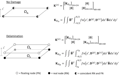
2.2.2 Floating Node Method

The enriched shell element uses the Floating Node Method (FNM) to enable discrete

repre-sentation of damage in a mesh by splitting elements where delaminations form. The FNM is described at length in [70]. It can be summarized briefly as follows. Extra DOF, “floating

nodes,” associated initially with zero stiffness, are embedded in an element formulation with

predefined connectivity. If a discontinuity forms (such as a delamination), the floating nodes can be activated and used to define subregions, ΩA and ΩB, within an element. The creation

of subregions does not modify the original global nodal definitions or DOF connectivity. In a

solution procedure, DOF associated with floating nodes that are not used are condensed out and not included in the numerical solution of the model.

Figure 2.4 is an illustration of a shell element formulation enriched with the FNM where a

(39)

accommodate multiple delaminations. Two states are shown, with and without the discontinuity. In the case where a delamination does not exist, the material integration is through the entire

laminate thickness, −h/2 to h/2. In the case where a discontinuity does exist, the material integration in thez0direction is split into two parts, one for each subregion, at thez0-coordinate of the delamination, zd. An element can be defined with as many floating nodes as desired if representation of more than one delamination is needed.

If an element is split into two or more subregions, each subregion stiffness matrix must undergo an offset transformation to account for the fact that the neutral axis of the subregion

is offset from that of the original element definition. The offset causes coupling of membrane

forces and nodal rotations in the subregion. This transformation is performed with an offset matrix and is given by

K0_Ω_i =T(off)TKΩiT

(off) _(2.54)

T(off) is the sum of a 24×24 identity matrix and off-diagonal terms given by T_1,5(off)=−d

T_2,4(off)=d T_7,11(off)=−d

T_8,10(off)=d (2.55)

T_13,17(off) =−d T_14,16(off) =d T_19,23(off) =−d T_20,22(off) =d

(40)

Ω

_A

= coincident RN and FN = floating node (FN) = real node (RN)

Ω

A

Ω

B

, , ′

/

′

, , ′

/ ′

, , ′

/

′ z̒

z̒

No Damage

Delamination

Figure 2.4 Floating Node Method.

2.2.3 Damage algorithm

An algorithm combining the shell element formulation, the FNM, and VCCT was created to simulate damage growth in a laminate.

2.2.3.1 Delamination growth

The Virtual Crack Closure Technique (VCCT) is used with the enriched shell to predict

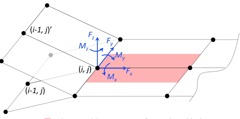
delam-ination growth after convergence of each increment in an analysis solution procedure (similar to Orifici et al [50]). Subregions in split shell elements are tied together at nodes along a

delamina-tion front. At each tied node along a delaminadelamina-tion front, energy release rate is calculated using

the tie forces and the nodal displacements in the crack wake. This is illustrated in Figure 2.5 for a delamination front node (i, j). The prime superscript identifies “upper” nodes. Equations for calculating energy release rate when using shell elements were determined by Wang et al. [60].

(41)

node (i, j) in Figure 2.5 as an example

GI = −1 2∆A

F_z(i,j)

w(i−1,j)0 −w(i−1,j)

+ (2.56)

M_x(i,j)θ_x(i−1,j)0 −θ(i_x−1,j)+

M_y(i,j)

θ(i_y−1,j)0−θ_y(i−1,j)

.

GII = −1 2∆A

F_x(i,j)

u(i−1,j)0 −u(i−1,j)

(2.57)

GIII = −1 2∆A

F_y(i,j)v(i−1,j)0−v(i−1,j)+ (2.58)

M_z(i,j)

θ_z(i−1,j)0−θ_z(i−1,j)

where ∆A is the change in crack area if the nodal tie is released. The moment terms go to zero if rotational DOF are not included in the ties. For cases where the element size ahead of a crack tip is different than the element size in the wake, a correction factor must be applied

to equations 53-55. Correction factors based on a 1/√r stress field singularity at the crack tip were derived by Rybicki and Kanninen [32]. If necessary, corrected values for energy release rate, designated by a prime superscript, can be obtained by

G0_I =GI

r

∆a1 ∆a2

(2.59)

G0II =GII

r

∆a1 ∆a2

(2.60)

G0_III =GIII

r

∆a1 ∆a2

(2.61)

(42)

F

_z

M

_y

F

_x

M

_x

F

_y

(

i

‐

1,

j

)’

(

i

‐

1,

j

)

(

i,

j

)

M

_z

= change in delamination area if tie is released (∆A)

Figure 2.5 Virtual Crack Closure Technique tie forces and nodal displacements.

and is given by

GT =GI+GII+GIII (2.62)

The value for GT is calculated at each delamination front node and compared to a critical value, Gc. If GT > Gc, then delamination growth is predicted and that nodal tie is released. Mixed-modeGc is calculated using the Benzeggah-Kenane equation [89]

Gc=GIc+ (GIIc−GIc)(GII/GT)ηBK (2.63)

whereGIc andGIIc are critical energy release rate for Mode I and Mode II cracks, respectively, and ηBK is an experimentally determined parameter.

Specifically, for the enriched shell formulation, elements are split in the vicinity of a

de-lamination front as shown in Figure 2.6. In an element formulation where a maximum of one

delamination can exist (i.e., four real nodes and four floating nodes), there are four possible damage states for an element, as shown in Figure 2.6: (1) No damage - floating nodes are

un-used; (2) element is split - all floating nodes are tied to corresponding real nodes; (3) element

(43)

= real node (RN) = floating node (FN) = RN tied to FN = RN & unused FN

(i, j) = node designation

GT(+x)≠ 0

GT(-y)= 0

GT(-x) = 0

GT(+y) = 0

y x

b b

(i, j) (i, j+1) (i, j-1)

(i+1, j)

(i-1, j)

= undamaged element

= split element ahead of crack tip w/all nodes tied = split element at crack tip w/one or more nodes tied = split element in wake of crack tip w/all nodes free = delamination front

(a) Isometric view

(b) plan view

(44)

As shown in Figure 2.6b, at a given delamination front node (i, j),GT is calculated along mesh lines in four directions. The maximumGT only is then used in the growth criterion. For delamination growth in non-physical or unlikely directions (such as −x or +/−y in Figure 2.6b), GT is calculated as approximately zero due to the nodes in what would be the crack wake being tied together and, therefore, numerically, delamination growth is eliminated as a

possibility. If an element has more than one delamination front (i.e., at different ply interfaces),

this same procedure is performed for each one.

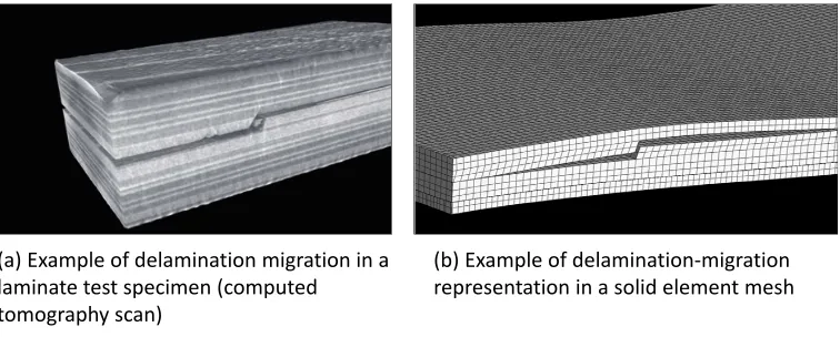
2.2.3.2 Delamination-migration: representation

Figure 2.7a shows a computed tomography scan of a composite laminate test specimen where

a delamination, after some initial growth, migrated through a ply via a transverse matrix crack

to a different interface where its growth continued. An example model shown in Figure 2.7b illustrates how this type of damage feature is traditionally represented in a finite element mesh.

When using shell elements, a different approach must be taken to represent out-of-plane damage

features.

(a) Example of delamination migration in a laminate test specimen (computed tomography scan)

(b) Example of delamination‐migration representation in a solid element mesh

Figure 2.7 Delamination migration in a test specimen and in a solid element mesh.

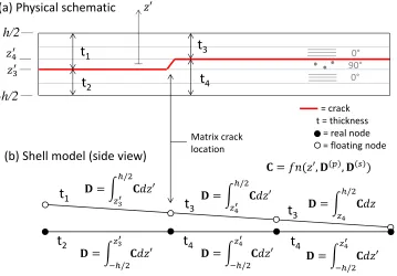
The physical schematic in Figure 2.8a shows a delamination-migration that has occurred in a cross-ply specimen (similar to the damage seen in Figure 2.7). Using the physical schematic

as a guide, Figure 2.8b shows how the transverse crack is represented in a shell mesh. The

(45)

the effect of the matrix crack is included in the model as a discontinuity in stiffness between elements. More specifically, in terms of the element formulation, there is a discontinuity from

one element to another in the z0 integration bounds in equations 22a-22d and in equation 2.27.

t

₁

t

₂

t

₃

t

₄

(a)

Physical

schematic

t

₁

t

₂

t

₃

t

₄

t

₃

t

₄

0° 90°

0°

(b)

Shell

model

(side

view)

-h/2

h/2

′ /

′ / ′

/

Matrix crack location

= crack t = thickness

= real node = floating node

′ / / ′, , ′

Figure 2.8 Representation of delamination migration in a shell mesh.

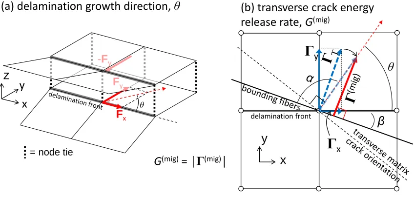
2.2.3.3 Delamination-migration: 2D prediction

A straightforward two-step criterion similar to that used by De Carvalho [49] is used to predict delamination-migration. O’Brien observed that many Mode I microcracks form ahead of a

shear delamination front in the resin-rich region at the ply interface where the delamination is located [90]. The first step of the delamination-migration prediction, Step I, is to determine the

orientation of th