domains containing conical singularities
Thesis by Zhiyi Li
In Partial Fulfillment of the Requirements for the Degree of
Doctor of Philosophy
California Institute of Technology Pasadena, California
2009
c
Acknowledgments
Abstract
Contents
Acknowledgments iii
Abstract iv
1 Introduction 1
1.1 Background . . . 2
1.2 Integral equation formulations . . . 5
1.2.1 Decomposition of the density function ν(x) . . . 8
1.3 A new approach to the conical singularity problem: Preliminary examples . . 9
1.3.1 Example: Numerical integration with a singular integrand . . . 9
1.3.2 Example: Resolution of a singular limit . . . 10
1.4 Outline of chapters . . . 12
2 Boundary Parameterization and the Fixed Partition of Unity 15 2.1 Overlapping patches Pk . . . . 16
2.2 Fixed POU function . . . 18
2.3 The parameterization for the region Sσ near the conical point . . . 22
3 On Singular Exponents, Singular Coefficients and Their Evaluation 25 3.1 Computation of the singular pair (qi, ai(θx)) . . . 27
3.1.1 Preliminary calculations . . . 27
3.1.2 Reduction to the infinite straight-cone case . . . 29
3.1.3 Evaluation of the singular pair . . . 31
3.2 Evaluation of−ai(θx)
2rxqi
+R
Sσ
∂G(x,x0)
∂nx ·
ai(θx0)
rqi
x0
dS(x0) forxclose to the conical point
O . . . 34
4 Discrete integral operator: trapezoidal rule, polar coordinates and graded meshes 38 4.1 Smooth integrands and trapezoidal rule . . . 40
4.2 Kernel singularity and polar coordinates . . . 43
4.2.1 Floating partition of unity . . . 43
4.2.2 Efficient interpolation scheme . . . 51
4.3 H¨older density singularity and graded meshes . . . 52
4.4 Evaluation of−ai(θx) 2rxqi ˆ ωP1(x) +R P1 ∂G(x,x0) ∂nx ai(θx0) rqi x0 ˆ ωP1(x0)dS(x0) . . . 60
5 The discrete linear system and accurate evaluation of disparate singular quantities 61 5.1 The overall discrete operator . . . 62
5.2 Discrete linear system . . . 63
5.3 Conical-point preconditioning . . . 64
6 Computational examples 69 6.1 Singular pairs: Numerical results . . . 76
6.2 Numerical solution for the circular- and elliptical-conical-point surfaces . . . 77
7 Conclusions 83
A Parameterizations of the patches Pk and the fixed POU functions 85
List of Figures
1.1 Left: Function √1
x. Middle: Change of variable function x =x(t). Right: The
integrand 1
x(t)12x
0(t) obtained after the change of variable x(t) . . . . 10
2.1 The surface ∂D with one conical point . . . 17
2.2 Patch P1 covers the area near the conical point . . . . 17
2.3 Patch P2 covers the area opposite to the conical point . . . . 17
2.4 Auxiliary function P(t, t0, t1) . . . 19
2.5 Values of the Fixed POU function ω1(x) on its support set (⊆ P1); in color code. 20 2.6 Values of the Fixed POU function ω1(x1 (u1, v1) on its domain H1; in color code. 20 2.7 Graph of the Fixed POU function ω1(x1 (u1, v1)) on its domain H1 . . . . 20
2.8 Color-coded values of the Fixed POU functionω2(x) on its support set on patch P2 . . . . 21
2.9 Color-coded values of the Fixed POU functionω2(x2(u2, v2)) on its support set in domain H2. . . . . 21
2.10 Graph of the Fixed POU function ω2(x2(u2, v2)) on its support set in domain H2. . . . 21
2.11 The straight-cone region Sσ (in red) near the conical point on the surface ∂D. 22 2.12 The parameters r, θ, φx near the conical point O. . . 23
4.1 Support of a floating POU function not crossing the boundaryv1 = 0 (displayed on the patch P1). . . . 46
4.2 Support of a floating POU function not crossing the boundaryv1 = 0 (displayed in H1). . . . . 46
4.4 Support of a floating POU function crossing the boundaryv1 = 0 (displayed in P1). . . . 47
4.5 Support of a floating POU function crossing the boundaryv1 = 0 (displayed in H1). . . . 47
4.6 Graph of a floating POU function whose support crosses the boundary v1 = 0. 47
4.7 Integrand in which a density function of the form 1
r0.28 is assumed, and without
using the floating POU factor. . . 49 4.8 Integrand including a density function r0.281 using the 1−ηx floating POU factor. 49
4.9 Integrand as a function of u1
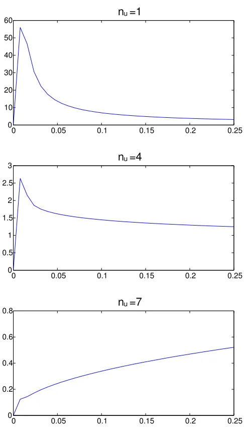
x0 for various values of nu. . . 56
4.10 For nu = 1 and r close to 0, the integrand containing the (1−ηx(x0)) factor
has a large peak around r0 = 0 that is not uniformly-integrable as r→0. . . . 57 4.11 Integrand containing the (1−ηx(x0)) factor and incorporating annu = 7 change
of variables. Clearly this change of variables effectively eliminates the r0 = 0 peak shown in Figure 4.10. . . 57 4.12 For nu = 1 and r close to 0, the integrand containing the ηx(x0) factor has a
large peak around r0 = 0 that is not uniformly-integrable as r →0. . . . 58 4.13 Integrand containing the ηx(x0) factor and incorporating an nu = 7 change of
variables. Clearly this change of variables effectively eliminates the r0 = 0 peak shown in Figure 4.12. . . 59
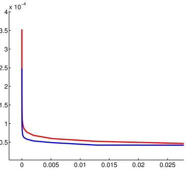
5.1 Error in the functionb arising from use of the un-preconditioned system; resid-ual tolerance = 10−12 . . . . 67
5.2 Same as Figure 5.1 but with residual tolerance = 10−14 . . . . 67
5.3 Same as Figure 5.1 but with residual tolerance = 10−16 . . . . 67
5.4 Red: error in the function b arising from use of the un-preconditioned system,
= 10−17. Blue: error in the function b arising from use of the preconditioned
system, = 10−8 (compare Table 5.1). . . . 68
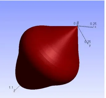
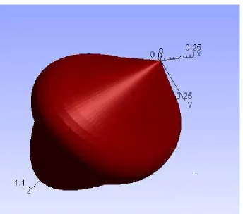
6.1 The circular-conical-point surface. . . 70 6.2 The elliptical-conical-point surface. . . 71 6.3 Bounded part b(x) of the solution for the right-hand-side ∂N(x)
∂n on the
6.4 Bounded partb(x) of the solution for the right-hand-side ∂N(x)
∂n on the
elliptical-conical-point surface. . . 73 6.5 Bounded partb(x) of the solution for the right-hand-side ∂Px0(x)
∂n on the
circular-conical-point surface. . . 74 6.6 Bounded partb(x) of the solution for the right-hand-side ∂Px0(x)
∂n on the
elliptical-conical-point surface. . . 75 6.7 Bounded part b(x) of the solution on the azimuthal lines zx = Const. for an
elliptical-conical-point body, and RHS ∂N∂n(x). . . 78 6.8 Bounded partb(x) of the solution on the polar line θx =π/64 for an
List of Tables
1.1 Error arising from the trapezoidal quadrature rule applied to the function √1
x
with and without the change of variables (COV)x=x(t), and usingN function values/quadrature points. . . 10
4.1 Errors arising from use of the trapezoidal quadrature for evaluation of the integral (4.20) using two values of the change-of-variables exponent nu. . . 56
4.2 Errors arising from use of the trapezoidal quadrature for evaluation of the integral (4.25) using two values of the change-of-variables exponent nu. . . 59
5.1 GMRES residual tolerances , number of iterations required to meet such tol-erances, and accuracy indicators for the un-preconditioned (table on the left) and preconditioned (table on the right) systems. . . 66
6.1 Errors in the numerical values of qi for a circular cone with apex angle π for
various numbers of discretization points Nsp. . . 77
6.2 Maximum error (0 ≤ θ ≤ 2π) in the numerical values of ai(θ) for a circular
cone with apex angle π for various numbers of discretization points Nsp. . . . 77
6.3 Errors (shown at selected mesh points close to the conical point) in the bounded part b(x) of the solution of an elliptical-conical-point problem with RHS ∂N(x)
∂n
obtained from a computational mesh containing 16×16 points per patch. . . 79 6.4 Errors (shown at selected mesh points close to the conical point) in the bounded
part b(x) of the solution of an elliptical-conical-point problem with RHS ∂N(x)
∂n
obtained from a computational mesh containing 32×32 points per patch. . . 79 6.5 Errors (shown at selected mesh points close to the conical point) in the bounded
part b(x) of the solution of an elliptical-conical-point problem with RHS ∂N(x)
∂n
6.6 Maximum errors and maximum function valuesbmax on various azimuthal lines
zx = Const. for the bounded part b(x) of the solution of an
elliptical-conical-point problem with RHS ∂N∂n(x) obtained from meshes of varying degrees of fineness. . . 80 6.7 Errors on the numerical values of the singular-term coefficients c1 and c2 for
an elliptical-conical-point problem with RHS ∂N∂n(x), obtained from meshes of varying degrees of fineness (the coefficients obtained from the finest (128×128) mesh are c1 = 19.197 and c2 =−42.1). . . 80 6.8 Maximum errors and maximum function valuesbmax on various azimuthal lines
zx = Const. for the bounded part b(x) of the solution of an
elliptical-conical-point problem with RHS ∂Px0(x)
∂n obtained from meshes of varying degrees of
fineness. . . 80 6.9 Maximum of the errors on the numerical values of the singular-term coefficients
c1andc2for an elliptical-conical-point problem with RHS ∂Px0(x)
∂n , obtained from
meshes of varying degrees of fineness (the exact singular coefficients are c1 = 0
and c2 = 0). . . 81 6.10 Maximum errors and maximum function valuesbmax on various azimuthal lines
zx = Const. for the bounded partb(x) of the solution of a circular-conical-point
problem with RHS ∂N∂n(x) obtained from meshes of varying degrees of fineness. 81 6.11 Maximum of the errors on the numerical values of the singular-term coefficients
c1 and c2 for an circular-conical-point problem with RHS ∂N∂n(x), obtained from meshes of varying degrees of fineness (the coefficients obtained from the finest (128×128) mesh are c1 =−23.00635 and c230.56074). . . 81 6.12 Maximum errors and maximum function valuesbmax on various azimuthal lines
zx = Const. for the bounded partb(x) of the solution of a circular-conical-point
problem with RHS ∂Px0(x)
∂n obtained from meshes of varying degrees of fineness. 81
6.13 Maximum of the errors on the numerical values of the singular-term coefficients
c1 andc2 for an circular-conical-point problem with RHS ∂Px0(x)
∂n , obtained from
6.14 Errors in the solution ve(x) of the exterior Neumann problem on an
elliptical-conical-point surface, at various points outside the body (characterized by their
rx and θx coordinates). . . 82
6.15 Errors in the solution ve(x) of the exterior Neumann problem for an
elliptical-conical-point surface, at points outside the body limiting atp1(−0.33,0.24,0.53) and p2(0.38,0,0.32). The corresponding solution values are ve(p1) = 1.54 and
Chapter 1
Introduction
The problem of evaluating numerical solutions of Partial Differential Equations (PDE) un-der conditions that give rise to solution singularities (such as reduced differentiability and even blow up of the solutions themselves) is one of fundamental importance in science and engineering. Yet, a wide variety of such problems have not been adequately addressed from a computational perspective. In this thesis we consider a central and prototypical problem of this type, namely, solution of Laplace’s equation in domains containing conical singularities. Many other problems in domains containing conical singularities, including problems of wave propagation and scattering, electromagnetics, diffraction, solid mechanics and acoustics, can be tackled by similar techniques; further, many of the ideas developed in this text can be applied to other types of geometric singularities, including edge and polyhedral singularities. As mentioned above, however, our presentation will be restricted to the fundamental exam-ple provided by the Laplace equation in domains which, containing conical singularities, are otherwise smooth.
1.1
Background
As indicated above, a wide variety of areas of science and engineering give rise to problems containing geometric singularities of the type considered in this thesis. In fracture mechanics, for example, treatments are often needed for interior and surface flaws that are often found in solid structures. Analysis leading to predictions of whether these flaws may grow and become liable to produce catastrophic failure of the structure, are, clearly, of great importance. Mathematically, the stress fieldσ, a quantity that derives from solution of a system of PDEs akin to Laplace’s equation, becomes infinite at the crack-tips—thus giving rise to singular problems closely related to the main model problem considered in this thesis [18, 21, 25, 35]. In aerodynamics, in turn, the problem of evaluating the flow around an airfoil is one of great interest. In an inviscid fluid, the speed of air around the trailing edge of a moving airfoil can be infinite. Of course, in a real fluid, air does not move infinitely fast, but strong viscous forces are caused near the trailing edge: vortexes are accumulated and carried along with the moving airfoil, until a stagnation point moves to the trailing edge, and the Kutta condition is satisfied. In any case, generally, solution of the Laplace equation in singular domains arising from airfoil and wing geometries is of significant importance in theoretical and computational aerodynamics [8, 28].
Problems of diffraction of acoustic and electromagnetic waves by domains containing ge-ometric singularities arise in a wide range of contexts—including optics, remote sensing, antenna design, electromagnetic compatibility, etc. In the optics case, for example, diffrac-tion effects such as those originating at geometric singularities set a fundamental limit to the resolution of camera, telescope, or microscope. It is to be noted that, as is the case in the Laplace problems considered in this thesis, at sharp edges of the diffracting obstacle, the electromagnetic field vectors become infinite [14, 41].
Refer-ence [30] provides a theoretical analysis of the behavior of solutions for Laplace equations in polyhedral domains.
Significant contributions regarding the numerical solutions of such problems have been put forward as well. For the sake of completenes we first mention references concerning 2D elliptic equations with singular boundaries, although, we must note, problems in 2D are significantly simpler than their 3D counterparts. Early 2D contributions, in which the problem is approached through use of spatially refined meshes in the singularity region in-clude [3, 4, 15–17]; References [20, 24, 29, 40], in turn, use singular basis functions as part of finite element spaces. A different approach, which is well suited to the two-dimensional context, is proposed in References [26, 44, 45]: A separation of the domain near the geomet-rical singularity is introduced, and “DtN” conditions are imposed on the artificial boundary. Other recent contributions include [38] (which gives a method for evaluation of the number of singular terms for a two-dimensional elasticity problem with two different wedge-shaped elastic materials bonded together along a common edge and subject to tractions on the boundary); Reference [46] (which uses the infinite element method to obtain singular solu-tions of the Helmholtz equation), and [36] (which, using the infinite element method, seeks solutions for composite-material problem with singular interfaces); References [2, 7] (which treat elliptic equations with boundary singularities using the singular complement method); Reference [23, 27] (which provides high-order integral equation methods for elliptic equa-tions), and Reference [23] (which provides a comparison of a method based on use of special basis functions with an approach based on adaptive mesh refinement); and finally, Refer-ence [33] (which treats the Maxwell equations with boundary singularities, using the Fourier finite element method).
an approximate asymptotic method, valid in the high-frequency regime, for evaluation of the scattering of a plane polarized electromagnetic wave by a perfectly conducting cone. Reference [31] studies the boundary element method for integral equations of the first kind in 2D and 3D for problems of scattering. Reference [34] treats the Maxwell equations with boundary singularities, using the Fourier finite element method.
As mentioned above, in this thesis we address one of the main problems in this area, namely, solutions of elliptic equations aroundconical singularities; as shown in what follows, our work resulted in solvers that can produce solution to 3D problems containing conical singularities with a high order of accuracy obtained. In detail, our work focuses on Laplace equation with constant coefficients;
∆u= 0 in D
u=f or ∂u
∂n =g on ∂D,
(1.1)
thesis give rise to significant improvements in the numerical accuracy of the singular compo-nents and the full solution—even for cases containing negative expocompo-nents for which integral densities blow up at the singular point. These integral densities correspond to physically
meaningful quantities such as solution derivatives or, in the electromagnetic case, to the electrical current itself. To the best of our knowledge, this is the first contribution enabling accurate numerical evaluation of such types of singularities for solution of PDEs in domains bounded by closed singular boundaries.
The approach introduced in this thesis is based on consideration of integral equations and algorithms that can provide high-order accuracy for approximation of singular integrals. To achieve such high accuracies our methods proceed by first splitting off the most singular part of the solution. These singular parts are determined by means of a novel (surface) nonlinear eigenvalue problem which, to the best of our knowledge, has not been considered previously. Our algorithm then proceeds to evaluate integrals whose integrands involve such singular functions. Evaluation of these integrals amounts to a rather challenging problem; in our approach these quantities are obtained, with high order accuracy, by means of appropriate series expansions we developed. With singular parts pulled out, the remaining relatively smooth(er) part of the solution can be computed by means of an application of high-order quadrature rules based on the use of graded meshes around the singular points. With this high order quadrature rule in place, our algorithm proceeds to formulate the full discrete linear-algebra problem, which is solved by means of the iterative linear-algebra solver GM-RES. As shown in Chapter 4, finally, a small modification of the integral operator can be used to reduce the number of iterations required by the iterative linear-algebra solver to fully separate the singular parts from the smooth parts of the solution.
1.2
Integral equation formulations
Laplace equations that are considered in this thesis, namely
∆ui = 0 in Di
ui = f on ∂D (Interior Dirichlet Problem) (1.2)
and
∆ve = 0 in De ∂ve
∂n = g on ∂D
(Exterior Neumann Problem). (1.3)
Here Di is a bounded region inR3; De is the exterior of Di: De =R3\Di; n is an exterior
normal to Di; ∂D is the common boundary of Di and De.
According to the method of boundary integral equations, the solutions ui and ve of the
boundary problems (1.2) and (1.3) can be represented as double-layer and single-layer po-tentials with densities µ and ν:
ui(x) =
Z
∂D
∂G(x,x0)
∂nx0
·µ(x0)dS(x0) (1.4)
ve(x) = Z
∂D
G(x,x0)·ν(x0)dS(x0) (1.5)
where G(x,x0) is the Green’s function of Laplace operator
G(x,x0) = 1
4π|x−x0|,
and where the functions µand ν are solutions to the following boundary integral equations on∂D:
−µ(2x)+
Z
∂D
∂G(x,x0)
∂nx0
·µ(x0)dS(x0) =f(x) for x∈∂D (1.6)
−ν(2x)+
Z
∂D
∂G(x,x0)
∂nx
·ν(x0)dS(x0) =g(x) forx∈∂D. (1.7)
problems:
µ=ue|∂D−f (1.8)
ν = (∂v
i
∂n)|∂D, (1.9)
where ue and vi are solutions of the conjugate problems
∆ue = 0 inDe, ∂u
e
∂n = ∂ui
∂n on∂D
∆vi = 0 inDi, vi =ve on∂D.
A proof of (1.8) and (1.9) can be found in [32].
The regularity properties (smoothness or lack thereof) of the solutions µ and ν deter-mines to a significant extent the order of accuracy of a numerical solver for equations (1.2) and (1.3)—since the accuracies delivered by quadrature rules themselves depend on the in-tegrand regularities. As is known, however, when the boundary ∂D has conical points, the integrands are not smooth around those points. For example, as shown in [32], the density function ν(x) in (1.7) tends to infinity at the conical point.
In what follows we develop a method for solution of PDE problems including a conical boundary point on the basis of equation (1.7). We point out that the Laplace equation with the Neumann boundary conditions can be solved by means of alternate integral equations, whose solution does not tend to infinity at the conical point. Indeed, the solution of the “direct” integral equation (see e.g., [9, 10]) equals the solution ve of the Neumann problem
and is thus bounded. In many circumstances, however, use of singular solutions and re-lated quantities is unavoidable. The simplest example of this involves the evaluation of the normal derivative of the solution vi of the interior Dirichlet problem which, according to
equation (1.9) tends to infinity at the conical point—since so does ν. The present approach thus allows one to evaluate this meaningful physical quantity; clearly, solution of the alter-nate equation followed by differentiation would give rise to very poor results. An additional example results from consideration of the Maxwell equations, which include an equivalent of
∂vi
∂n as a component of the unknown surface current along an edge. Thus, in addition to
around a conical point.
For simplicity, in this thesis we only consider a three dimensional body with one conical point, in a neighborhood of which the surface coincides with the boundary of a straight cone of arbitrary (smooth) cross section, as depicted in Figure 2.12. Generalization to a curved cone boundary surface should result as an extension of the method developed in this work.
1.2.1 Decomposition of the density function ν(x)
In equation (2.5) we define the coordinates (rx, θx) on the integration surface ∂D near the
conical pointO: with an appropriate interpretation, implicit in (2.5),rxdenotes the distance
[image:20.612.125.500.505.603.2]from the conical point O and θx is the azimuthal angle. These coordinates are depicted in
Figure 2.12.
According to [32], we have an asymptotic expansion forν(x) near the conical point:
ν(x) = X
i
ciai(θx)
rqi
x
ˆ
ωP1(x) +b(x), (1.10)
where
qi >0, (1.11)
and where the function b(x) is bounded throughout ∂D. (The definition for the terms in
equation (1.11) is in equation (3.1))
Using the decomposition in equation (1.10), the integral in equation (1.7) becomes
−ν(x)
2 +
Z
∂D
∂G(x,x0)
∂nx
·ν(x0)dS(x0)
=X
i
−ciai(θx)
2rqi
x
ˆ
ωP1(x) + Z
∂D
∂G(x,x0)
∂nx
· ciai(θx0)
rqi
x0
ˆ
ωP1(x0)dS(x0)
+
−b(2x)+
Z
∂D
∂G(x,x0)
∂nx
·b(x0)dS(x0)
.
(1.12)
In the following chapters we develop a number of procedures for accurate evaluation of the right hand side of equation (1.12); note that this requires, in particular, evaluation of a bounded difference of infinite quantities; see Section 1.3.2 below for a simple example in
1.3
A new approach to the conical singularity problem:
Prelimi-nary examples
To demonstrate, in simple settings, some of the main issues that arise as we address the main problem considered in this thesis, in this section we present two elementary introductory examples. The purpose of this section is thus to provide an indication of the nature of the algorithms developed in the following chapters.
1.3.1 Example: Numerical integration with a singular integrand
Let’s first consider an elementary integration problem:
Z 1
0
1
√xdx (1.13)
This is a finite integral with infinite integrand near x = 0. The integrand, f(x) = √1x is shown in Figure (1.1) Left. A direct application of a quadrature rule such as the trapezoidal rule results in slow convergence as shown in the second column of Table 1.1. In order to address this difficulty we follow [9]: we use a change of variables x = x(t), depicted in the middle portion of Figure 1.1, to obtain a new integrandf(x(t))x0(t) = √1
x(t)·x
0(t), depicted in Figure 1.1 Right. One important feature of x(t) is thatx(t) =tn with n >2 for tclose 0.
As a result of this property of x(t), the integrand becomes
ntn−1· 1 tn2
neart = 0. This new integrand is a smooth function, fornlarge enough this function vanishes as t → 0 together with several of its derivatives. The function x(t) increases smoothly to 1, and stays constant in an interval where t is close to 1. So x0(t) = 0 near t = 1 as well. Overall, the new integrand is smooth and vanishes near the two end points of the interval
t∈[0,1] as depicted in Figure 1.1 Right. Using the change of variablesx=x(t), the integral (1.13) becomes
Z 1
0
1
x(t)12
N error without COV error with COV
20 0.3016 0.0092
40 0.2184 -0.0014
80 0.1570 -6.3545e-6
160 0.1123 7.4472e-10
320 0.0801 2.4425e-15
Table 1.1: Error arising from the trapezoidal quadrature rule applied to the function √1x with and without
the change of variables (COV)x=x(t), and usingN function values/quadrature points.
0 0.2 0.4 0.6 0.8 1
0 5 10 15 20 25 30 35
x
f(x)
0 0.2 0.4 0.6 0.8 1
0 0.2 0.4 0.6 0.8 1
t
x(t)
0 0.2 0.4 0.6 0.8 1
0 2 4 6 8 10 12
t
f(x(t))x’(t)
Figure 1.1: Left: Function √1x. Middle: Change of variable function x = x(t). Right: The integrand 1
x(t)12x
0(t) obtained after the change of variablex(t)
The trapezoidal rule provides excellent convergence for this new integral, as shown in the third column of Table 1.1. Similar changes of variable will be used in our algorithms to tackle problems of integration of unbounded functions with finite integrals.
Remark 1.3.1. Changes of variables designed to produce smooth and periodic integrands
play major roles in the algorithms developed in this thesis. Indeed, we transform all singular
integrands into integrands that are smooth and periodic, for which the trapezoidal quadrature
rule is highly (spectrally) accurate.
1.3.2 Example: Resolution of a singular limit
Our next example brings up an issue that lies at the heart of the issues considered in this thesis.
We consider the problems of evaluating the limit
lim
as well as values of Fs(y) for very small y >0, where Fs is given by
Fs(y) =y−s−
Z 1
0
xys
(y+x2)32
dx, (1.16)
where the exponent s is determined by the requirement that the limit (1.15) must be finite. In the present case all three problems, the evaluation of s, the limit, and the function val-ues for small y can be solved easily through closed form integration; for the corresponding nonlinear eigenvalue problems considered in Section 3.1.3, in contrast, no exact integration can be performed, eigenfunctions are involved, and nonlinear equations must be solved—so that the simple closed-form manipulations presented in what follows need to be substituted by a sequence of numerical procedures. With a view to the analysis in Section 3.1.3, below we show that, even in the context of the simple example under consideration, use of numer-ical quadrature rule would not give rise to accurate determination of the exponent s, the limit (1.15) or values ofFs(y) for small values ofy.
Remark 1.3.2. In the context of our integral equation problem on surfaces containing conical
singularities, the need to evaluate integral quantities “very small values” of a parameter y
arises from the graded meshes used near the conical points: some of the sampling points we
use can be as close to the conical point as 10−8 or even 10−10 times the size of the surface
diameter.
We thus proceed with our highly idealized example: integrating with respect to x we obtain
Fs(y) = y−s−ys−
1
2 +ys(y+ 1)− 1
2 (1.17)
from which it is a simple matter to check that the condition
−s =s− 1
2,
ors = 14, is necessary and sufficient for the limit (1.15) to be finite. Having determined the exponent s = 1
4 we now seek to evaluate Fs(y) for small values
Fs(y) without recourse to the closed form expression of the integral
Z 1
0
xy41
(y+x2)32
dx. (1.18)
The integral (1.18) tends to ∞ as y → 0+, and, thus, a numerical evaluation of this quantity by means of a standard quadrature rule would produce inaccurate results. Further, the subtraction of two nearly infinite quantities as in equation (1.16) would give rise to significant cancellation errors, and, thus, additional accuracy loss.
An alternative approach we use can be demonstrated in the present example: taking into account the fact that
y−14 =
Z ∞
0
xy14
(y+x2)32dx,
and that, as a result,
y−14 −
Z 1
0
xy14
(y+x2)32dx=
Z ∞
1
xy14
(y+x2)32dx, (1.19)
we can evaluate F1/4(y) for small y by means of an expansion of the integrand: xy14
(y+x2)32 = y14 x2 ·
1 (1 + xy2)
3 2
= y
1 4
x2 ·(1−
1 1!
3 2(
y x2) +
1 2! 3 2 5 2( y x2)
2
− · · ·). (1.20)
In all we obtain
F1/4(y) =
Z ∞
1
xy14
(y+x2)32dx=y 1 4 − 1
1! 3 2
y1+14
3 + 1 2! 3 2 5 2
y2+14
5 − · · · (1.21)
The right hand side series in equation (1.21) converges very fast for the small values of ywe consider. Thus, instead of approximating an integral whose value is close to ∞, and then subtracting two nearly infinite quantities, the procedure described above evaluates the quan-tity (1.16) by means of the series (1.21), with high accuracy and at very low computational cost.
1.4
Outline of chapters
In Chapter 2 we describe our parametrization of the boundary surface ∂D. In order to discretize our integral equations with a high order of accuracy, we first make the integrand smooth and periodic on a parameter space by partitioning the integration problem by means of certain smooth and periodic functions.
In Chapter 3, we present novel methods to compute singular pairs (ai(θx), qi), which are
determined by the left hand side of the integral equation, and, thus, by the geometry of the conical surface. With (ai(θx), qi) computed, we develop methods to evaluate accurately the
quantities
−ai(θx)
2rqi
x
+
Z
∂D
∂G(x,x0)
∂nx
· ai(θ0) rqi
x0
dS(x0). (1.22)
This is a challenging issue since, as discussed in Section 1.3.2, as the target pointxapproaches
the conical point the overall integrand becomes more and more singular, in such a way that, regularizations similar to that considered in Section 1.3.1 do not suffice to produce acceptable accuracies. (As noted in Section 1.3.1, use of changes of variables give rise to useful regularization of infinite integrands, as long as the integrands admit a finite integral, of course. In the present case the integrals are finite, but tend to infinity as x approaches
the conical point—so that a change-of-variable regularization scheme becomes less and less useful, and ultimately completely losses all accuracy as x approaches the conical point.)
Using ideas demonstrated in Section 1.3.2, a methodology to address these difficulties is presented in Section 3.2.
In Chapter 4, we describe our discretization scheme for the integrals on surface∂Dthrough isolation of the integral kernel singularity, and application of the trapezoidal rule to every part of the integral. We shall see the discretization indeed exhibits high order of accuracy in any cases.
In Chapter 5, the discretization schemes introduced in previous chapters are used to produce a full discrete formulation for the boundary integral equation (1.7) using ci and
b(x) as unknowns (see equation (1.12)). In this formulation, we utilize the singular pairs
(ai(θx), qi) computed previously, and the unknown b(x) is determined for all points on a
mesh on the surface ∂D.
Chapter 2
Boundary Parameterization and the
Fixed Partition of Unity
We seek to solve numerically the boundary integral equation (1.7) on the surface∂D. In this thesis, the surface ∂D is assumed to be the boundary of a three dimensional body D with a conical point O; throughout this work we assume that in a neighborhood of the conical point O the surface ∂D coincides with the boundary of a straight cone defined by a given cross sectional curve, see Figure 2.12, and that, with exception of the conical singularity,∂D
is a smooth surface.
Our goal is to solve a discretized version of equation (1.7) by means of an iterative linear-algebra solver; the main difficulty to achieve this goal lies in producing an accurate algorithm for evaluation of the operator on the left hand side of equation (1.7), and the associated integral
Z
∂D
∂G(x,x0)
∂nx
·ν(x0)dS(x0), (2.1)
for given points x∈ ∂D. (As mentioned in Section 1.3.2, for xclose to the conical point O
the complete operator on the left hand side of equation (1.7) must be evaluated as a unit, and not as a difference of two large quantities.)
To evaluate these operators, we use an adequate representation of the boundary surface
2.1
Overlapping patches
P
kSince the surface ∂D generally cannot be represented by a single parametrization, in order to evaluate the integral in equation (2.1) we follow the approach [6], which is based on use of local coordinate parametrizations and Partitions of Unity (POU).
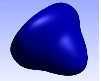
According to the POU method, we describe the boundary surface ∂D using several over-lapping coordinates patches Pk, k = 1, . . . , n. In particular, to describe a surface with a
conical point, such as that shown in Figure 2.1, we use two patches: one patch, which we call P1 and displayed in blue in Figure 2.2, contains the region near the conical point O;
the second patch, which contains the complement of the first patch P1 and overlaps with P1, is called P2 and shown in red in Figure 2.3. Note the existence of a significant region of
overlap between these two patches.
The coordinates patches Pk, (k = 1,2) are assumed to satisfy the following conditions:
1. Each patch Pk is an open set within ∂D, and the union P1 ∪ P2 covers all of ∂D.
2. Each patch Pk is the image of a coordinate open set Hk, contained in a plane. The
coordinate set Hk is mapped to patch Pk via a parametrization
xk=xk(uk, vk) defined for (uk, vk)∈ Hk, k = 1,2. (2.2)
A curve O1 ∈ H1 is mapped to the conical point O through the k = 1 parametrization
defined in equation (2.2).
3. The parametrization in equation (2.2) is smoothly invertible, and the vector product
Vk(uk, vk) = ∂x
k
∂uk ×
∂xk
∂vk
is bounded away from zero in (H1 \ O1)∪ H2. We assume Vk is an outward normal, so
that the outward unit normal on Pk is given by
nk = V
k
|Vk|.
We use the open sets Hk and its coordinates (uk, vk) to evaluate the integral operator on
Figure 2.1: The surface∂Dwith one conical point
Figure 2.2: PatchP1 covers the area near the conical point
[image:29.612.221.395.495.635.2]and patches we use for the numerical examples in this thesis. The corresponding coordinate domains are Hk = [0,1]×[0,1],(k = 1,2).
2.2
Fixed POU function
According to the POU method, the overlapping patches Pk are used to decompose the
integral on surface ∂D into the sum of two integrals over Pk, k = 1,2. To achieve this decomposition, we use a set of partition of unity functions {ωk(x);k = 1,2} subordinated
to these overlapping patches Pk, k = 1,2.
Specifically, we use the set of functions {ωk(x);k= 1,2}, such that
1. ωk(x) is defined, smooth, and nonnegative on ∂D;
2. ωk(x) vanishes outside Pk;
3.
2
X
k=1
ωk = 1 throughout∂D. (2.3)
This pair of smooth functions will be referred to as the “fixed” partition of unity, in contrast with certain “floating” partitions of unity that are introduced in Chapter 4.
Using patch parametrizations xk(uk, vk) and POU functions ωk(x) as discussed above,
the integral in equation (2.1) can be decomposed as
Z
∂D
∂G(x,x0)
∂nx
ν(x0)dS(x0)
=
2
X
k0=1
Z
Pk0
∂G(x,x0)
∂nx
ν(x0)ωk
0
(x0)dS(x0)
=
2
X
k0=1
Z
Hk0
∂G(x,xk0(uk0
x0, v
k0
x0))
∂nx
ν(xk
0 (ukx00, v
k0
x0))
·Jk0(uk 0
x0, v
k0
x0)ω
k0
(xk0(uk0
x0, v
k0
x0))du
k0
x0dv
k0
x0. (2.4)
Here, Jk0(uk 0
x0, v
k0
x0) is the Jacobian of the parametrization (u
k0
x0, v
k0
x0) for the patch P
k0 .
Clearly, on the non-overlapping regions of a patch Pk, ωk must be equal to 1; further,
the fixed POU function ωk(x) should vanish smoothly towards the boundaries of the k-th
0 0.2 0.4 0.6 0.8 1 0
0.2 0.4 0.6 0.8 1
t
P(t,t
0
,t1
)
t=t0 t=t1
Figure 2.4: Auxiliary function P(t, t0, t1)
the function P(t, t0, t1) depicted in Figure 2.4. The analytic form of function P(t, t0, t1) is described in Appendix A. In particular we note from Figure 2.4 that P(t < t0, t0, t1) = 1;P(t > t1, t0, t1) = 0, and P(t, t0, t1) decays smoothly from 1 to 0 as t goes from t0 tot1.
In Figures 2.5 and 2.6, we show, in color code, the values of the fixed POU functionω1(x)
on the patch P1 and the domain H1, respectively; the values ω1(x1(u1, v1)) as a function of
the coordinates (u1, v1) are shown in Figure 2.7. In Figures 2.8 and 2.9, in turn, we display the
functionω2(x2(u2, v2)) as a function of the parameters (u2, v2). These figures show the fixed
POU functions as well as the manner in which each one of the two dimensional coordinate domains Hk is mapped onto the patch Pk in three dimensional space. (The analytic forms
of the fixed POU functions and the coordinates mappings xk(uk, vk) are further discussed in
Section 4.1 and described in Appendix A.)
The main feature of these fixed POU functions is that ωk(x) = 1 in the center of the
patches, and ωk(x) smoothly decays to 0 towards the boundary of the patch Pk, where the
patches overlap. On patchP1,ω1(x) = 1 forxnear the conical pointO, and smoothly decays
to 0 as the distance to the conical point O increases. Clearly, the region {x;ω1(x)<1} on
Figure 2.5: Values of the Fixed POU function ω1(x) on its support set (⊆ P1); in color code.
Figure 2.6: Values of the Fixed POU function ω1(x1(u1, v1) on its domainH1; in color code.
0
0.5
1
0 2 4 6 0 0.5 1
u1
2π v1
ω
1
Figure 2.8: Color-coded values of the Fixed POU functionω2(x) on its support set on patchP2
Figure 2.9: Color-coded values of the Fixed POU functionω2(x2(u2, v2)) on its support set in domainH2.
0
0.5
1
0 0.5
1 0 0.5 1
u2
v2
ω
2
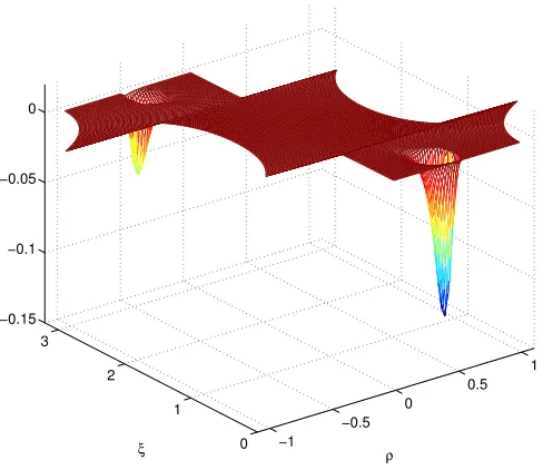
Figure 2.11: The straight-cone regionSσ (in red) near the conical point on the surface∂D.
2.3
The parameterization for the region
S
σnear the conical point
As mentioned above, in this thesis, we assume the surface ∂D coincides with the boundary of an infinite straight cone near the conical point O. More precisely, we assume there is a number σ > 0 such that the region Sσ of all points on ∂D whose distance to the conical
point is less than or equal to σ which coincides with the boundary of a straight cone with a smooth cross section; see Figure 2.11 for a depiction in which Sσ is a portion of an elliptic
cone. Note that the region Sσ is generally bounded by a non-planar curve: the boundary
line lies on a plane only whenSσ is a section of a circular cone.
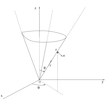
To represent points x inSσ we use the spherical coordinates (rx, θx, φx) with azimuthal
plane parallel to the x−y plane and with origin at the conical pointO:
xx = rxsinφx(θx) cosθx
yx = rxsinφx(θx) sinθx
zx = rxcosφx(θx);
(2.5)
Figure 2.5 displays a pointxon a straight cone surface with spherical coordinates (rx, θx, φx).
O
θ
r x
n
x
y z
[image:35.612.134.492.206.532.2]φ
are given by (rx, θx, φx(θx)):
Sσ ={(rx, θx, φx(θx)); 0< rx < σ},
for a certain smooth function φx. As an example, in Appendix A, we present the function
φx(θx) for the surface of a straight elliptic cone.
Remark 2.3.1. In this thesis we often use the notation x(rx, θx, φx(θx)) for a point in the
region Sσ. The coordinates (rx, θx) are most useful in our discussion of the computation of
singular terms in Chapter 3.
Remark 2.3.2. Throughout this thesis we assume (as we may) that the parameterσis small enough so that Sσ does not overlap with patch P2. Consequently, the fixed POU function
ω1(x) equals 1 for x∈S
Chapter 3
On Singular Exponents, Singular
Coefficients and Their Evaluation
In Reference [32], it is shown that the density functionν(x) in equation (1.7) can be expressed
in the form
ν(x) = ˆω
P1(x) X
i
ciai(θx)
rqi
x
+b(x) (3.1)
with
qi >0, (3.2)
where |b(x)| . rp as r → 0 for some p > 0. We call qi the “singular exponent”, ai the
“singular coefficient”, and (qi, ai(θx)) the “singular pair”. Here rx and θx are the
spher-ical coordinates of the point x as described in Section 2.3, and, denoting by (u1
x, v
1
x) the
coordinates of x in the domain H1 we have set
ˆ
ωP1(x) =
0 x∈∂D\ P1
ω1(u1
x, v
1
x) x∈ P
1,
(3.3)
whereω1(u1x, v
1
x) is the fixed POU function of patchP
1. Note that, according to the definition
Using the decomposition (3.1), the integral equation (1.7) becomes
−ν(x)
2 +
Z
∂D
∂G(x,x0)
∂nx
·ν(x0)dS(x0)
=X
i
−1
2
ciai(θx)
rqi
x
ˆ
ωP1(x) + Z
P1
∂G(x,x0)
∂nx
ciai(θx0)
rqi
x0
ˆ
ωP1(x0)dS(x0)
+
−b(2x) +
Z
∂D
∂G(x,x0)
∂nx
·b(x0)dS(x0)
=g(x).
(3.4)
In equation (3.4), the integrand ciai(θx)
rxqi
ˆ
ωP1(x) is only integrated on patch P1 since the
windowing function ˆωP1(x) vanishes outside P1.
The rest of this Chapter is organized as follows: In Section 3.1, we describe a numerical method for the evaluation of singular exponentsqi and coefficients ai(θx) for a given straight
cone boundary surface of arbitrary cross section. As we will see, the determination of the singular pair (qi, ai(θx)) is independent of the explicit form of the right hand side g(x) in the
integral equation (3.4).
In Section 3.2, in turn, we describe a method for the evaluation of
−12ai(θx)
rqi
x
ˆ
ωP1(x) + Z
Sσ
∂G(x,x0)
∂nx
ai(θx0)
rqi
x0
ˆ
ωP1(x0)dS(x0) (3.5)
in cases for which x is either close to or coincides with the conical point O. (Note that the
integration domain in equation (3.5) is region Sσ, which is contained in but is different from
patch P1.) In Chapter 4, we describe a method for numerical evaluation of the integral in
the complementary region P1\S
σ.
Both our method for evaluation of singular pairs presented in Section 3.1 and the proce-dure described in Section 3.2 to evaluate the sum in equation 3.5 are essential elements of our overall algorithm. The former element allows us to isolate the most singular terms in our integral equation formulation. The latter element, on the other hand, which is closely related to the simplified example presented in Section 1.3.2, provides a means to produce bounded quantities that result as differences of quantities that tend to ∞ asx tends to the
3.1
Computation of the singular pair
(
q
i, a
i(
θ
x))
The evaluation of singular pairs proceeds through a reduction to the case of an infinite straight cone, as shown in the following three subsections.
3.1.1 Preliminary calculations
The right hand side of the integral equation (3.4) is a given function g(x) which in this
thesis is assumed to be bounded and continuous: this function coincides with the boundary condition in equation (1.3). The left hand side of the integral equation (3.4), on the other hand, may be expressed as the sum of a quantity involving singular terms
X
i
−ciai(θx)
2rqi
x
ˆ
ωP1(x) + Z
P1
∂G(x,x0)
∂nx
·ciai(θx0)
rqi
x0
ˆ
ωP1(x0)dS(x0)
(3.6)
and a quantity involving (more) regular terms
−b(2x) +
Z
∂D
∂G(x,x0)
∂nx
·b(x0)dS(x0). (3.7)
Asx tends to the conical pointO, both terms in equation (3.7) have finite values.
There-fore, in order for the left hand side in equation (3.4) to remain bounded as x tends to
the conical point (as they should, since the right hand side g(x) does), the singular pairs
(qi, ai(θx)) should satisfy the following condition:
lim
x→O
X
i
−ciai(θx)
2rqi
x
ˆ
ωP1(x) + Z
P1
∂G(x,x0)
∂nx
·ciai(θx0)
rqi
x0
ˆ
ωP1(x0)dS(x0)
<∞. (3.8)
Considering the terms under the summation symbol in equation (3.6), we note that, since the coordinate rx tends to 0 as the point x tends to the conical pointO, we have
−12ciai(θx)
rqi
x
ˆ
ωP1(x)∼ 1
rqi
x
→ ∞ asx→O.
As shown in Section 3.1.4, we have the following asymptotic formula for the integral con-taining the singular integrand term,
Z
P1
∂G(x,x0)
∂nx
· ciai(θx0)
rqi
x0
ˆ
ωP1(x0)dS(x0)∼ 1
rqi
x
It follows that, assuming, as we may, that the exponents qi are pairwise different,
Z
P1
∂G(x,x0)
∂nx
· ciai(θx0)
rqi
x0
ˆ
ωP1(x0)dS(x0) and ciai(θ
x)
rqi
x
ˆ
ωP1(x)
are the only terms in equation (3.4) that tend to∞ like 1
rxqi
asx tends to O. Consequently,
the condition in equation (3.8) becomes: for each i, singular pair (qi, ai(θx)) should satisfy
the condition
lim
x→O
−ai(θx)
2rqi
x
ˆ
ωP1(x) + Z
P1
∂G(x,x0)
∂nx
·ai(θx0)
rqi
x0
ˆ
ωP1(x0)dS(x0)
<∞. (3.10)
Notice the common factor ci (cf. equation (3.8)) has been removed at this stage.
Re-expressing the boundary integral in equation (3.10) as a sum of two integrals, one over the region Sσ and the other one over its complement P1 \Sσ, the condition (3.10) becomes
lim
x→O
−ai(θx)
2rqi
x
+
Z
Sσ
∂G(x,x0)
∂nx
· ai(θx0)
rqi
x0
dS(x0)
<∞ (3.11)
since, for x∈Sσ, ˆω
P1(x) = 1 and since the integral Z
P1\S σ
∂G(x,x0)
∂nx
· ai(θx0)
rqi
x0
ˆ
ωP1(x0)dS(x0) (3.12)
is a smooth function for x∈ Sσ.
In order to evaluate singular pairs (qi, ai(θx)) on the basis of the condition (3.11), we use
the coordinates (rx, θx) described in Section 2.3 as integration variables; condition (3.11)
then reads
lim
x→O
−ai(θx)
2rqi
x
+
Z σ
0
Z 2π
0
∂G(x,x0)
∂nx
(rx, rx0, θx, θx0)·
ai(θx0)
rqi
x0
Jr,θ(rx0, θx0)dθx0drx0
<∞
(3.13)
where
Jr,θ(rx, θx) =rx
r
(dφx
dθx
)2+ sin2φ
x (3.14)
in the region Sσ, the integration kernel is given by
∂G(x,x0)
∂nx
(rx, rx0, θx, θx0)
= 1 4π
rx0[cosφx0sin
2φ
x−sinφx0sin(θx−θx0)
dφx
dθx −sinφ
x0sinφxcosφxcos(θx−θx0)]
[r2
x+r
2
x0−2rxrx0(cosφxcosφx0 + sinφxsinφx0cos(θx−θx0))]
3 2
.
(3.15)
3.1.2 Reduction to the infinite straight-cone case
To proceed with the evaluation of singular pairs, we re-express the rx0-integral in
equa-tion (3.13) in the form
Z σ
0 ·
drx0 = (
Z ∞
0 −
Z ∞
σ
)·drx0 (3.16)
and we use the explicit forms (3.14) and (3.15) of the functions
∂G(x,x0)
∂nx
(rx, rx0, θx, θx0) and Jr,θ(rx, θx)
for the integral betweenσ and ∞. Integrating first with respect toθx0 and then with respect
torx0 we obtain
Z ∞
σ
Z 2π
0
∂G(x,x0)
∂nx
(rx, rx0, θx, θx0)·
ciai(θx0)
rqi
x0
Jr,θ(rx0, θx0)dθx0drx0
=
Z 2π
0
q
(dφx0
dθx0
)2+ sin2φ
x0
q
(dφx
dθx)
2+ sin2φ
x
ciai(θx0)·
(cosφx0sin
2φ
x−sinφx0sin(θx−θx0)
dφx
dθx
−sinφx0sinφxcosφxcos(θx−θx0))·
Z ∞
σ
r2−qi
x0
[r2
x+r
2
x0 −2rrx0(cosφxcosφx0 + sinφxsinφx0cos(θx−θx0))]
3 2
drx0dθx0.
(3.17)
x= rx0
rx, and we obtain
Z ∞
σ
r2−qi
x0
[r2
x+r
2
x0 −2rrx0(cosφxcosφx0 + sinφxsinφx0cos(θx−θx0))]
3 2
drx0
= 1
rqi
x
Z ∞
σ rx
x2−qi
[x2+ 1−2x(cosφ
xcosφx0 + sinφxsinφx0cos(θx −θx0))]
3 2
dx
= 1
q·σqi +O(rx).
(3.18)
The last equality results from the largex Laurent expansion 1
[x2+ 1−2x(cosφ
xcosφx0 + sinφxsinφx0cos(θx−θx0))]
3 2
= 1
x3(1 +O(
1
x)). (3.19)
The expansion in equation (3.19) is applicable to equation (3.18) for x close to O, so that
rx is small and
σ
rx is large.
Equations (3.18) and (3.19) show that the absolute value of the integral with respect to
rx0 in equation (3.17) is bounded by a finite constant that is independent ofθx andθx0 (recall
that φx and φx0 are functions of θx and θx0, respectively, cf. equation (2.5)). Since all θx
and θx0 dependent terms are also finite in the integral in equation (3.17), the full integral in
equation (3.17) is uniformly bounded as x tends to the conical point O:
lim
x→O
Z ∞
σ
Z 2π
0
∂G(x,x0)
∂nx
(rx, rx0, θx, θx0)·
ai(θx0)
rqi
x0
Jr,θ(rx0, θx0)dθx0drx0 <∞. (3.20)
Combining equations (3.13) and (3.20) we obtain
lim
x→O
−ai(θx)
2rqi
x
+
Z ∞
0
Z 2π
0
∂G(x,x0)
∂nx
(rx, rx0, θx, θx0)·
ai(θx0)
rqi
x0
Jr,θ(rx0, θx0)dθx0drx0
<∞,
(3.21)
or equivalently,
lim
x→O
1
rqi
x
−ai(θx)
2 +
Z ∞
0
Z 2π
0
∂G(x,x0)
∂nx
(rx, rx0, θx, θx0)·ai(θx0)
rqi
x
rqi
x0
Jr,θ(rx0, θx0)dθx0drx0
<∞.
(3.22)
3.1.3 Evaluation of the singular pair
The expression in equation (3.22) equals the product of 1
rxqi
with the quantity
−ai(θx)
2 +
Z ∞
0
Z 2π
0
∂G(x,x0)
∂nx
(rx, rx0, θx, θx0)·ai(θx0)
rqi
x
rqi
x0
Jr,θ(rx0, θx0)dθx0drx0
=
−
ai(θx)
2 +
Z 2π
0
Z ∞
0
q
(dφx0
dθx0
)2+ sin2φ
x0
q
(dφx
dθx)
2+ sin2φ
x
ai(θx0)
x2−qi(cosφ
x0sin
2φ
x−sinφx0sin(θx−θx0)
dφx
dθx −sinφ
x0sinφxcosφxcos(θx −θx0))
[x2+ 1−2x(cosφ
xcosφx0 + sinφxsinφx0cos(θx−θx0))]
3 2 dxdθx0),
(3.23)
where, once again, we have used the explicit forms (3.14) and (3.15) and the change of variablesx= rx
rx0
. Clearly, the quantity in equation (3.23) is independent of rx. Thus, for its
product with term 1
rqix
in equation (3.22) to remain finite in the limit as x→O (rx →0), it
is necessary that the expressions in equation (3.23) equal 0:
−ai(θx)
2 +
Z ∞
0
Z 2π
0
∂G(x,x0)
∂nx
(rx, rx0, θx, θx0)·ai(θx0)
rqi
x
rqi
x0
Jr,θ(rx0, θx0)dθx0drx0 = 0. (3.24)
Using the notation
Kq(c) =
Z ∞
0
x2−q
(x2+ 1−2xc)32dx, (3.25)
this condition can be expressed as the following equation for the singular pairs (qi, ai(θx)):
−ai(θx)
2 +
Z 2π
0
q
(dφx0
dθx0
)2+ sin2φ
x0
q
(dφx
dθx)
2+ sin2φ
x
ai(θx0)Kqi(cosφxcosφx0 + sinφxsinφx0cos(θx−θx0))
(cosφx0sin
2φ
x−sinφx0sin(θx−θx0)
dφx
dθx
−sinφx0sinφxcosφxcos(θx−θx0))dθx0
= 0.
(3.26)
Remark 3.1.1. The function Kq(c) in equation (3.25) can be computed analytically and
Mathematica.
Equation (3.26) determines the singular pairs (qi, ai(θx)). The exponents qi are those
quantities for which equation (3.26) admits nonzero homogeneous solutions ai(θx). In order
to solve this “nonlinear eigenvalue problem” numerically we discretize equation (3.26) using the trapezoidal rule, and thus obtain the following finite dimensional homogeneous linear system for the approximation of each exponent qi and discretization {aji, j = 1, . . . , Nsp} of
ai(θx):
1 2a
j
i+
1 4π
Nsp
X
j0=1
(Kqi(cosφ(θj) cosφ(θj0) + sinφ(θj) sinφ(θj0) cos(θj −θj0))·
[cosφ(θj0) sin2φ(θj) + sinφ(θj0) sin(θj0 −θj)
dφ dθ(θj) −sinφ(θj0) sinφ(θj) cosφ(θj) cos(θj0 −θj)]·
q
(dθdφ
x0
(θj0))2 + sin2φ(θj0)
q
(dφdθ(θj))2+ sin2φ(θj)
aji0
= 0 forj = 1. . . Nsp.
(3.27)
Here Nsp is the number of integration points we use to discretize equation (3.26), and aji is
the numerical approximation of the value ai(θj). The numerical values of the quantities qi
are determined as those for which the matrix associated with equation (3.27) admits 0 as an eigenvalue, and the values {aji} are the corresponding eigenvectors.
Analytical forms for the singular pairs (qi, ai(θx)) of cones with circular cross sections
are given in Reference [32]; using these analytical forms in Chapter 6 we demonstrate the accuracy of the approximations (qi,{aji, j = 1, . . . , Nsp}) resulting from equation (3.27). Of
course, the procedure described above is valid for conical points of arbitrary cross section.
Remark 3.1.2. Using the quantities {aji, j = 1, . . . , Nsp}, we can use an interpolation
al-gorithm to obtain approximations to the function ai(θx) for arbitrary angles θx. (Note that
given the periodic nature of functionai(θx), a high order of accuracy for the interpolation can
be achieved by means of Fourier series and FFTs). Thus an approximation to the singular
term ai(θx)
rqix
3.1.4 Asymptotic behavior of the integral in equation (3.9)
In Section 3.1.1 we used the asymptotic behavior (3.9) of the integral
Z
P1
∂G(x,x0)
∂nx
· ciai(θx0)
rqi
x0
ˆ
ωP1(x0)dS(x0)∼ 1
rqi
x
as x→O;
here we provide a proof of this relation. Considering the splitP1 = (P1\S
σ)∪Sσ as in equations (3.11) and (3.12), focusing first
on the integral on Sσ, and recalling equation (3.16), we obtain
Z
Sσ
∂G(x,x0)
∂nx
· ciai(θx0)
rqi
x0
dS(x0)
=( Z ∞ 0 − Z ∞ σ )
Z 2π
0
∂G(x,x0)
∂nx
(rx, rx0, θx, θx0)·
ciai(θx0)
rqi
x0
Jr,θ(rx0, θx0)dθx0drx0
= 1
rqi
x
Z ∞
0
Z 2π
0
∂G(x,x0)
∂nx
(rx, rx0, θx, θx0)·ciai(θx0)
rqi
x
rqi
x0
Jr,θ(rx0, θx0)dθx0drx0
−
Z ∞
σ
Z 2π
0
∂G(x,x0)
∂nx
(rx, rx0, θx, θx0)·
ciai(θx0)
rqi
x0
Jr,θ(rx0, θx0)dθx0drx0.
(3.28)
Recalling equations (3.20) and (3.26), we note that
Z ∞
σ
Z 2π
0
∂G(x,x0)
∂nx
(rx, rx0, θx, θx0)·
ciai(θx0)
rqi
x0
Jr,θ(rx0, θx0)dθx0drx0
is uniformly bounded, and that
1
rqi
x
Z ∞
0
Z 2π
0
∂G(x,x0)
∂nx
(rx, rx0, θx, θx0)·ciai(θx0)
rqi
x
rqi
x0
Jr,θ(rx0, θx0)dθx0drx0 =
ciai(θx)
2rqi
x
.
As a result we obtain
Z
Sσ
∂G(x,x0)
∂nx
· ciai(θx0)
rqi
x0
dS(x0)
=ciai(θx)
2rqi
x
−
Z ∞
σ
Z 2π
0
∂G(x,x0)
∂nx
(rx, rx0, θx, θx0)·
ciai(θx0)
rqi
x0
Jr,θ(rx0, θx0)dθx0drx0
∼ciai(θx)
2rqi
x
∼ r1qi
x
as x→O.
Since the integral
Z
P1\Sσ
∂G(x,x0)
∂nx
· ciai(θx0)
rqi
x0
ˆ
ωP1(x0)dS(x0)
is a smooth function when x∈Sσ, the relation used in equation (3.9), namely Z
P1
∂G(x,x0)
∂nx
· ciai(θx0)
rqi
x0
ˆ
ωP1(x0)dS(x0)∼ 1
rqi
x
as x→O, (3.30)
follows directly.
3.2
Evaluation of
−
ai(θx)2rqix
+
R
Sσ
∂G(x,x0)
∂nx
·
ai(θx0)
rxqi0
dS
(
x
0)
for
x
close to the
conical point
O
To complete our formulation for the integral equation (3.4), we need to provide approximate numerical methods for the evaluation of all the terms of the left hand side operator. In Section 3.1, we computed the singular pair (qi, ai(θx)), and we showed that the integral
R
Sσ
∂G(x,x0)
∂nx ·
ai(θx0)
rxqi0
dS(x0) tends to ∞ as x tends to the conical point O. Clearly, therefore,
a straightforward quadrature rule would not evaluate this integral accurately, and, further the difference of the two associated infinite quantities, which should remain bounded, would give rise to significant cancellation errors and numerical instability.
Based on the fact that the sum
−ai(θx)
2 +
Z
Sσ
∂G(x,x0)
∂nx
· ai(θx0)
rqi
x0
dS(x0) (3.31)
remains bounded (a condition which we used to determine the singular pairs (qi, ai(θx))), in
this section, we provide an indirect method for evaluation of this sum for x either close to
or at the conical point O. In Chapter 4, in turn, we describe methods for evaluation of all the other terms on the left hand side of the integral equation (3.4), including the integral with the singular term integrands in region P1\S
σ,
Z
P1\Sσ
∂G(x,x0)
∂nx
· ai(θx0)
rqi
x0
ˆ
ωP1(x0)dS(x0). (3.32)
Remark 3.2.1. The sum in equation (3.31) does not include the (constant) coefficient ci of
and is an unknown that needs to be solved for as part of the full discrete formulation. Note
that, in particular, the evaluation procedure described in this section does not depend in any
way on the right hand side g(x).
To evaluate (3.31) we first express the surface integral in equation (3.31) in terms of the spherical coordinates (rx0, θx0):
−ai(θx)
2rqi
x
+
Z σ
0
Z 2π
0
∂G(x,x0)
∂nx
(rx, rx0, θx, θx0)·
ai(θx0)
rqi
x0
Jr,θ(rx0, θx0)dθx0drx0. (3.33)
Then we re-express therx0-integral in the form
Z σ
0 · drx0 =
Z ∞
0 · drx0 −
Z ∞
σ ·
drx0,
so that equation (3.33) becomes
− ai(θx)
2rqi
x
+
Z σ
0
Z 2π
0
∂G(x,x0)
∂nx
(rx, rx0, θx, θx0)·
ai(θx0)
rqi
x0
Jr,θ(rx0, θx0)dθx0drx0
=−ai(θx)
2rqi
x + ( Z ∞ 0 − Z ∞ σ )
Z 2π
0
∂G(x,x0)
∂nx
(rx, rx0, θx, θx0)·
ai(θx0)
rqi
x0
Jr,θ(rx0, θx0)dθx0drx0.
(3.34)
Taking into account equation (3.24) (which we used in Section 3.1 to compute the singular pairs) and the explicit forms (3.14) of the Jacobian Jr,θ(rx, θx) and (3.15) of the integration
kernel ∂G(x,x0)
∂nx (r
x, rx0, θx, θx0), equation (3.34) becomes
− ai(θx)
2rqi
x
+
Z σ
0
Z 2π
0
∂G(x,x0)
∂nx
(rx, rx0, θx, θx0)·
ai(θx0)
rqi
x0
Jr,θ(rx0, θx0)dθx0drx0
= 1
rqi
x
Z 2π
0 (− Z ∞ σ rx ) q
(dφx0
dθx0
)2+ sin2φ
x0
q
(dφx
dθx)
2+ sin2φ
x
ai(θx0)
x2−qi(cosφ
x0sin
2φ
x−sinφx0sin(θx−θx0)
dφx
dθx −sinφ
x0sinφxcosφxcos(θx−θx0))
[x2+ 1−2x[cosφ
xcosφx0 + sinφxsinφx0cos(θx−θx0)]]
3 2 dxdθx0,
(3.35)
where once again we used the change of variable x= rx0
rx.
equa-tion (3.35), our algorithms use the trapezoidal rule to produce highly accurate approxima-tions of the corresponding θx0-integral. To obtain the x-integral in a half-line, in turn, we
do not resort to classic