An Experimental Evaluation of the Performance of the Amorphous Silicon PV Array on the NCSU AFV Garage

(1)

Abstract

CHRISTY, DANIEL WILLIAM. An Experimental Evaluation of the Performance of the Amorphous Silicon PV Array on the NCSU AFV Garage. (Under the direction of Dr. Herbert M. Eckerlin.)

A comprehensive performance test has been conducted on the 3 kW amorphous

silicon photovoltaic (PV) system on the roof of the Alternative Fuel Vehicle Garage of the

North Carolina Solar Center. The purpose of this testing program was to measure the

performance of the PV system, to determine if any deterioration has occurred over the past

three years since installation, and to evaluate the performance of the individual circuits that

makeup the PV system.

Test conducted on the individual circuits of the PV system showed significant

differences. This is particularly true for the two different solar panel models, which were

installed using different techniques. Numerous tests were conducted on these circuits to

isolate the problem. The current-voltage curves of the factory-laminated panels were much

worse than the self-laminated panels. No cause of the poor performance could be

definitively established. Discussions with the PV panel manufacturer are continuing to

identify the cause of the variation in PV circuit performance.

Comparisons made to performance data recorded in 2003-2004 show a similar kWh

production over 3-month periods, this is encouraging. However, comparisons between

global irradiance and AC power production show a 9% reduction in power production.

Continued research is recommended to further evaluate the circuit issues and to

study how PV panel temperatures can be reduced so as to improve over PV system

(2)

An Experimental Evaluation of the Performance of the Amorphous Silicon PV Array on the NCSU AFV Garage

by

DANIEL WILLIAM CHRISTY

A thesis submitted to the Graduate Faculty of North Carolina State University

in partial fulfillment of the requirements for the Degree of

Master of Science

MECHANICAL ENGINEERING

Raleigh, North Carolina

2007

APPROVED BY:

_________________________ _________________________ Dr. James W. Leach Dr. Tarek Echekki

________________________________ Dr. Herbert M. Eckerlin

(3)

Biography

Dan Christy was born in Chardon, OH on February 26, 1980. Dan moved to

Warrenton, Virginia in 1989 and attended and graduated from Fauquier High School in

1998. He then attended the University of Virginia receiving a bachelors of science in

aerospace engineering and graduated in 2002. Starting in June of 2002 Dan started working

for Directed Vapor Technologies International. He stayed there until May of 2005 when he

moved to Raleigh, NC to attend North Carolina State University work towards a master’s of

science in mechanical engineering. While attending NC State University he worked for the

(4)

Acknowledgements

I’d like to thank Shawn Fitzpatrick for all of his help building the data logging

system and answering all the many questions I had while working on the project and

writing the thesis. I’d like to thank Dr. Herbert Eckerlin for all of his constructive feedback

(5)

List of Tables

Table 1. Electrical Specifications ... 3

Table 2. Data Logger Equipment List ... 14

Table 3. Noon Inverter Efficiency Data... 31

Table 4. Individual Panel Voltages... 34

Table 5. Short Circuit Current Comparison... 43

Table 6. Energy Production Over Each Study... 45

Table 7. Shading Data... 46

Table 8. Conclusion Summary... 50

Table 9. Example Data Logger Output... 55

Table 10. PV Log... 60

(8)

List of Figures

Figure 1. Alternative Fuels Vehicle Garage ... 2

Figure 2. Electrical Diagram of Photovoltaic System Layout (McGuffy 167) ... 3

Figure 3. Outdoor Power Conditioning Equipment... 4

Figure 4. Combiner Box ... 5

Figure 5. Current Monitoring Enclosure... 6

Figure 6. n-type/p-type Junction with Load Shown ... 10

Figure 7. Current-Voltage Curve ... 11

Figure 8. Voltage vs. Power... 12

Figure 9. Data Logging System Schematic ... 13

Figure 10. Data Logging System ... 14

Figure 11. Data Logger Channels ... 16

Figure 12. Eppley and Li-Cor Pyranometers ... 17

Figure 13. AC-Power Measurement Diagram ... 19

Figure 14. Current-Voltage Curve Tracer... 26

Figure 15. Solar Irradiance versus AC Power Output ... 29

Figure 16. Solar Irradiance on a Clear Day and a Scattered Clouds Day... 30

Figure 17. AC Power Output for Solar Conditions shown in Figure 16 ... 30

Figure 18. Variation of Inverter Efficiency as a Function of Inverter Output (AC Power) . 32 Figure 19. Energy Production for Individual Circuit on January 2, 2007 ... 33

Figure 20. Max Power Point Voltage for Individual Circuits... 35

(9)

Figure 22. Current-Voltage Curve for Circuits D and F... 37

Figure 23. Power-Voltage Curve for Circuits D and F... 38

Figure 24. Current-Voltage Curve for Individual Panels within Circuit F... 39

Figure 25. 2003 to 2004 Solar Radiation versus AC Power Output... 41

Figure 26. 2007 Solar Radiation versus AC Power Output... 41

Figure 27. Circuit A Short Circuit Current Comparison ... 43

Figure 28. Hypothetical Shading Effects on Panel Current-Voltage Curve ... 47

Figure 29. Shading Effect on Power-Voltage Curve ... 47

Figure 30. Solar Panel Specification Sheet Page 1 ... 63

(10)

1. Introduction and Background

The amorphous silicon photovoltaic system investigated in this study is located in

Raleigh, North Carolina on the campus of North Carolina State University. The

photovoltaic system was installed on the roof of the Alternative Fuels Vehicle (AFV)

Garage that is a part of the North Carolina Solar Center. The garage is located next to the

NCSU Solar House.

The purpose of this investigation was to determine the performance of the amorphous

silicon PV array, to compare its present performance with 2003-2004 performance, to

determine if any deterioration had occurred over the past three years, and to evaluate

differences in individual circuit performance.

The report begins with a description of the solar array and its components already in

place. An overview of how photovoltaic panel work is explained next. A data collection

system to monitor parameters of the array was built so that the objectives above could be

achieved. This system is described in detail. Many experiments were performed to answer

the questions about the system’s operational performance and results and conclusions are

explained in detail.

1.1. Solar Array

The photovoltaic system includes two types of solar panels in this system. There

are sixteen Uni-Solar SSR-128J panels and eight Uni-Solar PVL-128B panels. The main

difference between the two types is the PVL-128B panels were field laminated to the roof

(11)

the garage with all 24 panels. The eight PVL-128B panels are on the left or west side of the

roof while the sixteen SSR-128J panels are on the right or east side of the garage.

Figure 1. Alternative Fuels Vehicle Garage

The sixteen SSR-128J panels had been in storage for over 3 yearsbefore they were

placed on the roof. The eight PVL-128B panels were purchased shortly before the entire

system was installed on the roof and were glued to the metal roof just prior to roof

installation.

The two types of panels have identical electrical specifications. Table 1 shows the

specifications given by the manufacturer. One part of this study was to compare the actual

performance with the manufacturer’s specifications. Each panel has a rated power of 128

watts and with 24 panels the system has about a 3 kW peak power rating. This rating tells

(12)

Table 1. Electrical Specifications

Rated Power (Watts) 128 Operating Voltage (Volts) 33.0 Operating Current (Amps) 3.88 Open Circuit Voltage (Volts) 47.6 Short Circuit Current (Amps) 4.80

The array has pairs of panels (called circuits) in series with one another to raise the

output voltage of the system to a level accepted by the inverter. The resulting 12 circuits

are then placed in parallel with each other to combine the current output. Figure 2 shows an

electrical diagram of the entire system.

(13)

Several components of the system convert DC power produced by the panels into

AC power that can be used by the AFV garage or returned to the general power grid. The

inverter is the primary piece of equipment for power conditioning and is the device that

actually does the DC to AC power conversion. Figure 3 shows some of the power

conditioning and energy measurement equipment on the outside wall of the AFV garage.

Each of these components is also shown in Figure 2.

Figure 3. Outdoor Power Conditioning Equipment

The inverter plays an important role in the operation of the PV system in that it

holds the entire PV array at a certain DC voltage. This max power voltage is found by

sweeping a range of voltages to find the maximum power output. This is called maximum

power point tracking or MPPT. The inverter displays the MPPT voltage (i.e. the voltage

(14)

Additional information that is displayed on the inverter includes the operating DC

voltage, AC voltage, AC power output, watt-hours produced for the day, time the inverter

has been operating for the day and the lifetime kWh produced. These values were recorded

several times during the study (see Appendix B for log). The readings were also used

during experiments to see how the array was operating under various solar conditions.

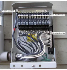
Other system components include the combiner box and the service panel. The

combiner box is where the wiring from the twelve circuits are combined together to go into

the inverter. The service panel is the circuit breaker for the garage and the point where

power comes into the garage or out to the grid (depending on the solar resource). Figure 4

shows the inside of the combiner box. The combiner box contains two bus bars where the

12 circuits are combined. The circuit switches are used to turn off individual panels.

(15)

The existing monitoring components include two kWh meters and a current

monitoring box in the attic of the garage. The first kWh meter measures the total energy

produced by the solar array. The second kWh meter is the power company meter and

measures the net energy used by the garage (i.e., utility power minus PV power provided to

the grid). Figure 3 above shows the location of the two kWh meters.

The current monitoring box in the attic has twelve 10 mΩ resistors. The current for

each circuit is sent through one of these resistors. A voltage drop can be measured across

each 10 mΩ resistor and using Ohm’s law, the current can be calculated.

R V I

R I V

= ⋅ =

Figure 5 shows the current monitoring enclosure.

(16)

1.2. Photovoltaic Effect

Some background into how the photovoltaic effect works can be useful in

understanding the basics for some of the experiments conducted in this study. A discussion

of semiconductors is necessary in order to explain how a solar cell works. An explanation

of how the photovoltaic effect works gives a science-oriented background. The final

subsection explains how a solar cell uses the photovoltaic effect to produce power.

1.2.1. Semiconductors

All atoms have an outer layer of electrons called the valence band. These are the

electrons that interact with other atoms. Conductors have few electrons in the valence band

and insulators have full valence bands. Semiconductors are in between these two. For

example, silicon (the most common base material for photovoltaic cells) has four valence

electrons with eight electrons needed to fill its particular valence band (Goswami 412).

If electrons in the valence band of an atom are energized they can reach into a

higher energy band (called the conduction band). Electrons here need only a small push to

be released from the atom entirely. The energy difference between the valence band and

the conduction band is called the band gap. Conductors have very low band gap energies

and insulators have very high band gaps. Semiconductors are in between the two

(Goswami 412).

Semiconductors used in solar cells are doped or extrinsic semiconductors. Doped

semiconductors have small amounts of impurities added to them. An n-type semiconductor

has an impurity with more electrons in its valence band than the base materials of the

(17)

appears to have an excess of electrons. A p-type semiconductor has fewer electrons in its

valence band than the base material and its overall structure seems to have fewer electrons

than expected. In other words, the p-type has holes for electrons to fill. By themselves,

n-type and p-n-type semiconductors are electrically neutral (Goswami 412).

If an n-type and a p-type semiconductor are placed next to each other, some of the

“excess” electrons from n-type semiconductor go to fill the “holes” in the p-type

semiconductor. This causes the n-type side to become electrically positive and the p-type

side to become electrically negative. This negative charge assists in directing electrons

through an external load. The electrons are freed by the photovoltaic effect (Goswami

414).

1.2.2. Photovoltaic Effect

The photovoltaic effect drives photovoltaic panels in that it causes electrons to move

into the conduction band of an atom when the electron absorbs enough solar energy. The

amount of energy needed is determined by the band gap of the material the photovoltaic

cell is made of. A single photon of light must carry the required energy to push the electron

through the band gap. If the photon energy is too small, the energy is converted into heat.

Likewise, if the energy of the photon exceeds the band gap energy, the extra energy is

converted into heat. One photon cannot energize two electrons. This is the primary reason

solar cells are relatively inefficient (Goswami 415).

Once the electron has reached the conduction band, it has potential to generate

(18)

electron will simply go back to its original energy state giving up energy as heat. This is

where the junction between the n-type and p-type semiconductors becomes important.

1.2.3. Solar Cells

When sunlight strikes the n-type side of the solar cell, it energizes the electrons.

When this occurs, the electrons have three choices. They can go through the external load,

recombine with the holes in the n-type semiconductor, or move towards the p-type

semiconductor side of the solar cell. The goal is to get the electrons to go through the

external load. The negative charge of the p-type semiconductor side restricts the movement

in that direction. The n-type semiconductor layer is made very thin and this limits the

opportunities the electron has to recombine (Goswami 415). Thus, the only option left is

the external load, which will generate the electrical power.

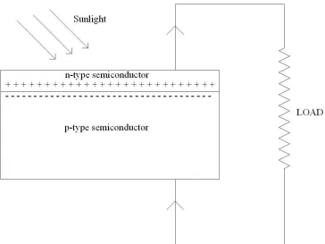
Figure 6 shows a simple diagram of the n-type/p-type junction. Right at the

interface between the two is the difference in electrical charge. The n-type side gives up

electrons to the p-type side. The sunlight will strike the n-type side energizing electrons,

(19)

Figure 6. n-type/p-type Junction with Load Shown

1.3. Current-Voltage Curves

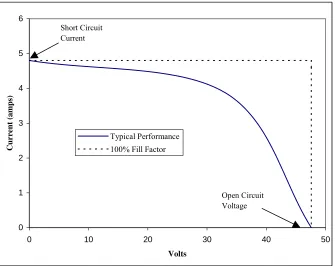
The performance of a solar panel can be judged by using a current-voltage or I-V

graph. A current-voltage curve shows the current and voltage a solar panel produces over

all resistances. The short circuit current and the open circuit voltage make up the ends of

the curve. Figure 7 shows an approximation of the rated performance of the panels

involved in this study in full sun. Important values from the graph include the short circuit

current (the y-intercept), and the open circuit voltage (the x-intercept). These values are

easily measurable and give a point of comparison between panels of the same type. These

values help in determining the possible degradation of the panels over time and for

(20)

0 1 2 3 4 5 6

0 10 20 30 40 5

Volts

Current (amps)

0 Typical Performance

100% Fill Factor Short Circuit

Current

Open Circuit Voltage

Figure 7. Current-Voltage Curve

Figure 7 shows a second plot with the open circuit voltage and the short circuit

current forming a rectangle. This is called 100% fill factor. The fill factor of a panel is

defined as the percentage of the box that is filled by the actual current-voltage curve. A

higher fill factor indicates a better performing panel.

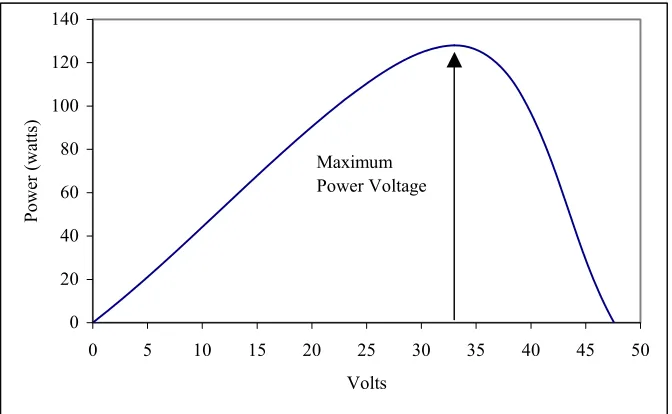
Figure 8 shows the voltage-power graph corresponding to Figure 7. The curve

shows how the power varies with voltage by simply multiplying the voltage and current at

each point on the I-V plot. This graph is used to determine the max power point, which in

(21)

0 20 40 60 80 100 120 140

0 5 10 15 20 25 30 35 40 45 50

Volts

Power (watts)

Maximum Power Voltage

Figure 8. Voltage vs. Power

1.4. Previous Work

The solar array was installed and made operational on November 13, 2003. A

performance study had been performed on the array from November 13, 2003 through April

9, 2004. The focus of the study was to analyze the relationship between the panel short

circuit current and the global irradiance. The study concluded that the ratio between short

circuit current and solar irradiance was 0.004184 amps per watt per square meter. Thus, for

a solar irradiance of 1000 watts per square meter, each circuit would yield a short circuit

current of 4.184 amps (Stanley). Additional data was collected at that time. Some of this

data was used in the present study to determine if the performance of the PV system had

(22)

2. Data Collection System

The heart of the data collection system is a Campbell Scientific CR10X data logger.

All of the data collection and initial storage takes place in this device. Data collected

includes solar intensity, AC power, DC voltage, current through circuits, ambient

temperature, and panel temperature (Appendix A shows example data output and the data

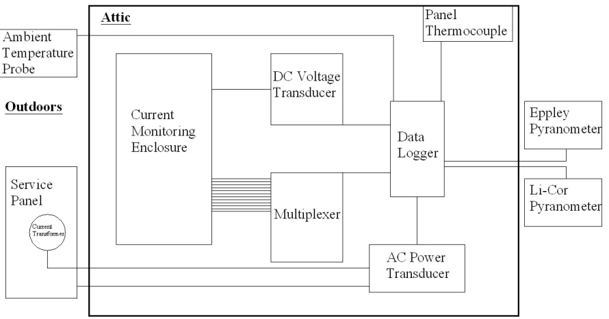
logger program. Figure 9 shows the schematic of the data logging system.

Figure 9. Data Logging System Schematic

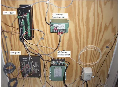
Figure 10 shows a photograph of a portion of data logging system in place in the

attic of the AFV garage. Included are the Ohio Semitronics DC voltage and AC power

measurement devices. Inputs not shown in the figure include the two pyranometers, the

thermocouple measuring panel temperature and the 107 temperature probe measuring

(23)

Figure 10. Data Logging System

Table 2 shows manufacturers and model numbers for the equipment used in the data

logging system.

Table 2. Data Logger Equipment List

Equipment Manufacturer Model No.

Data Logger Campbell Scientific CR10X

Multiplexer Campbell Scientific AM416 Voltage Transducer Ohio Semitronics VT7

Power Transducer Ohio Semitronics GWV5 Pyranometer 1 Eppley PSP

(24)

2.1. Data Logger

The Campbell Scientific CR10X data logger has twelve voltage inputs that can be

used for twelve single ended measurements or six differential voltage measurements. The

setup used a mixture of measurement types. A multiplexer was used to expand the

available channels. A multiplexer combines several channels of data down to one.

Figure 11 shows the setup of the channel inputs to the data logger. The DC Voltage

(3H), AC Power (3L), and the two pyranometers (4L, 5H) are all single-ended voltage

measurements. They are all also connected to the analog ground. The thermocouple

reference (4H) and the 107-temperature probe (5L) are single ended voltage measurements,

but they also are connected to an excitation voltage and analog ground. The single

thermocouple (6H, 6L) is used to measure the temperature on the back of a solar panel and

requires two of the twelve channels.

The multiplexer takes up four channels (1H, 1L, 2H, 2L) and has additional

connections to the data logger for power and controls. These include a 12V line, a ground,

and two control voltages. The multiplexer takes 12 differential voltages and outputs them

one at a time to the data logger. The control voltages change the differential voltage that is

(25)

Figure 11. Data Logger Channels

The data logger program was set up to take a data point from each instrument every

30 seconds. This data would then be averaged every 15 minutes and that data point would

be stored in the data logger. From time to time, the data stored would be downloaded to a

laptop for analysis. For certain tests, the storage time was reduced to one minute. This was

done to get more frequent data points.

2.2. Pyranometers

The pyranometers measure the solar intensity in watts per square meter. Two

different pyranometers were employed, an Eppley and a Li-Cor. The pyranometers were

mounted at the same angle of the roof at the bottom-west side of the roof. The two

pyranometers measure different sections of the solar spectrum and were used as a check

against each other. Figure 12 shows the two pyranometers mounted on the garage in the

plane of the roofline. The Eppley pyranometer is the larger device on the right and the

(26)

Figure 12. Eppley and Li-Cor Pyranometers

The Eppley pyranometer produces a voltage signal proportional to the solar

intensity, which is then converted with a multiplier into the correct units. The multiplier

used was 124.82

mV m

watts/ 2. This value comes from a calibration done by NREL (National

Renewable Energy Laboratory).

The Li-Cor pyranometer uses a small photovoltaic sensor to measure the solar

intensity and outputs a current proportional to the solar intensity. The current is sent

through a 147 ohm resistor and the data logger measures the voltage drop across the

resistor. The solar intensity measured is proportional to the current output of the

pyranometer multiplied by the constant shown below.

Output Current

Amp watt/m 12.55x10

Intensity Solar

2

6 _⋅

(27)

This current is sent through a resistor and using Ohm’s law, the current output can be determined. 147Ω Drop Voltage Output Current 147Ω Output Current Drop Voltage = ⋅ =

Combining two equations gives the power output in a form proportional to the voltage

output. Output) (mV 85.374 Intensity Solar 147Ω Drop Voltage Amp watt/m 12.55x10 Intensity

Solar 6 2

⋅ =

Thus 85.374 is the multiplier used in the data logger program to determine the Li-Cor

measured solar flux.

2.3. DC Voltage

The DC voltage of the system is measured using an Ohio Semitronics voltage

transducer (model # VT7). The VT7 receives the DC voltage from the current monitoring

enclosure in the attic of the AFV garage and converts it to a current output. This current

passes through a 2000-ohm resistor and the data logger measures the voltage drop across

that resistor.

2.4. AC Power

The inverter converts DC power into AC power that can be fed to the power grid.

An Ohio Semitronics GWV5 power transducer measures the AC power and outputs a

(28)

The available monitoring equipment however has some limitations. The power

transducer measures power up to 1000 watts and the solar array is capable of generating up

to 2500 watts. The data logger accepts voltages up to 2.5 volts while the power transducer

produces 5 volts at the top of its range. The power transducer produces 0-5 volts over a

range of 0-1000 watts. Since the data logger can only accept 2.5 volts, the maximum power

the transducer can measure is 500 watts. A current transformer was used to bring the

current going into the power transducer within allowable limits.

The voltage measurement is a direct measurement between the two lines going out

to the power grid. The current measurement is done with a current transformer using three

turns on the primary. This allows a finer resolution of the power to be determined without

bringing the voltage output of the power transducer to a level too high for the data logger.

Figure 13 shows a diagram of how the AC power is measured.

(29)

The following set of equations show the calculations used to determine the

multiplier used to convert the voltage output from the power transducer to units of power.

The actual power output is the AC voltage multiplied by the AC current. Three turns on the

primary were used so the current transformer input (ICTInput) should be three times the actual

current. AC CTInput AC AC I 3 I I V Power ⋅ = ⋅ =

The current transformer will output a 5 amp current for a 100 amp input giving a ratio of

input to output of 20:1.

20 I I_CTOutput = CTInput

In order to get the ratio of measured power to actual power, a few substitutions had to be

made. The equations below show one of the substitutions required to determine the

measured power. CTOutput AC AC CTOutput I V Measured Power I 20 3 I ⋅ = = Then, AC AC I 20 3 V Measured

Power = ⋅

Finally the ratio of measured power to actually power can be determined with a third

substitution using the original power equation.

Power 20

3 Measured

(30)

The power transducer outputs a voltage range of 0-5V over a 0-1000W power input. The

equation below shows the constant needed to convert from the voltage into the data logger

to the power measured.

mV 5000

Watts 1000 Read Voltage Power

20

3 _⋅ ₌ _⋅

A final combination of these last two equations gives the constant needed to convert the

data logger voltage into the actual power.

Voltage Logger

Data 333 . 1

Power= ⋅

With this information a multiplier of 1.333 was added into the data logger program in order

for it to output the data in units of power.

2.5. Panel Currents

The 24 panels on the roof are tied together in pairs in order to generate a voltage

that the inverter can accept. In the current monitoring enclosure in the attic, the current from each circuit is sent through a 10 mΩ current shunt (see Figure 5). By measuring the

voltage drop across the shunt, the current through each circuit can be determined.

With this information, the performance of the solar array can be evaluated. Any

differences in the current outputs of each circuit would indicate that all the panels are not

operating at expected output.

Using the sum of the twelve currents and the array DC voltage, a DC power can be

calculated. A comparison of the DC power to the AC power would give a measure of

(31)

2.6. Temperature Measurements

Temperature measurements were taken of the ambient air temperature and the PV

array. A 107-temperature probe measured the ambient air temperature and the PV array

temperature was measured by a thermocouple on the back of a single panel. The

107-temperature probe was placed underneath the side roof overhand to protect the probe from

rain. The probe was placed inside a radiation shield to prevent any sunlight from

interfering with the temperature measurement.

A thermocouple was place on the back of one of the solar panels to measure the

panel temperature. Temperature has a significant effect on photovoltaic performance.

(32)

3. Experiments

Several questions were raised after looking at the initial data from the data logging

system. Experiments were designed to answer the following questions:

- Has panel performance changed from three years ago?

- Do the individual circuits have different maximum power operating

voltages?

- What is the shape of the current-voltage curve for a good panel and a poor

performing circuit?

- How much effect does shading have on panel performance?

Each experiment discussed below attempted to answer one of these questions. The

results from the experiments are shown in the next chapter.

All comparisons made were done using identical instruments. Several methods of

measuring the solar intensity were used and care was taken to only compare this data

against data taken using the same instrument.

3.1. Open Circuit Voltage and Short Circuit Current

The open circuit voltage (Voc) and the short circuit current (Isc) were measured in a

previous study conducted from November 2003 to March 2004. To check for degradation

similar measurements were made during January and February of 2007 (Appendix C shows

an example data set).

To perform these experiments, all of the circuit breaker switches in the combiner box

(33)

voltage was measured for each of the twelve circuits independently. The measurement was

between the positive voltage coming into the combiner box and the negative bus bar in the

combiner box.

The short circuit current was measured by short circuiting the two bus bars in the

combiner box. Instead of the current leaving the combiner box and going to the inverter, all

of the current went through the ammeter, which was the shorting device. Each breaker was

turned on individually so only the current from one circuit was measured at a time. In

between each current reading, a solar irradiance measurement was taken using a handheld

pyranometer. Since the short circuit current is dependent on the amount of solar irradiance,

frequent measurements of the solar irradiance were taken to ensure reliable data.

In addition to the short circuit current and the open circuit voltage, all the information

from the inverter was recorded just before this particular experiment was conducted. This

includes the operating voltage and AC power output. In addition to the inverter data,

weather conditions, ambient temperature and panel temperatures were also recorded.

3.2. Circuit Power Point Tests

An investigation into the operating status of each circuit involved turning off 11 out

of 12 of the circuits. This allowed the inverter to find the maximum operating voltage for

each circuit rather than having to compromise by finding the maximum operating voltage

for the whole array. The readings recorded from the inverter display included the

maximum power point voltage (Vmpp), the DC voltage, and the AC power output. The solar

(34)

To perform this test, one of the twelve circuits was turned on for five minutes. The

data logger was set to store data points every minute (instead of every 15 minutes) in order

to get readings at the same time as the inverter readings. This allowed time for the inverter

to search for the maximum power point. Then the inverter readings were recorded.

During this experiment, some of the circuits produced a very low power output,

even in full sun. It is important to note that the inverter efficiency decreases at lower power

inputs.

3.3. Current-Voltage Plot Test

A current-voltage plot was generated by connecting the solar panels to a rheostat

(i.e. a variable resistor) instead of sending the power to the inverter. This resistance can be

varied between 6 Ω - 28Ω. A plot of voltage versus the current provides a good indication

of panel performance. Refer to Figure 7 to see a typical curve.

Figure 14 shows the setup of the current-voltage curve tracer. The two leads from

the solar panels come in from the bottom. The current then flows through the two resistors

and the ammeter. The ammeter is required to close the circuit. The voltage meter measures

the voltage drop across the two resistors. The resistance is varied using the coarse and fine

(35)

Figure 14. Current-Voltage Curve Tracer

3.4. Shading Tests

Shading can have a dramatic effect on PV system performance. Each panel contains

twenty-two 13.25” x 9.5” solar cells. Experiments were conducted under five different cell

shading levels defined below:

- unshaded

- ¼ cell shaded

- ½ cell shaded

- 1 cell shaded

- 1 ½ cell shaded

These levels shade from 0 to 6.8% of the total panel. For most tests, both panels in the

(36)

panels was covered. Data for each test was recorded with the data logging system on

one-minute intervals.

The current generated by each circuit was the most important parameter. Dividing

this recorded current by the pyranometer reading normalized the data to current per unit of

solar irradiance. This allows direct comparisons between data points and accounts for any

variation in solar intensity. The day chosen for the test was also a clear day around noon

when the solar irradiance fluctuates the least. An average normalized value for the

unshaded condition was used as the frame of reference to generate percentage values. The

unshaded condition was considered maximum current.

⎟⎟ ⎠ ⎞ ⎜⎜ ⎝ ⎛ = ₂ meter watts amps Value Normalized Reading r Pyranomete Current Panel Power Maximum of Percent Conditions Unshaded for Value Normalize Average Value Normalized ₌

The percent of maximum values can then be compared to each other. Comparisons are

(37)

4. Results, Conclusions and Recommendations

4.1. Effect of Solar Flux on Array Performance

Data was collected over a period of several months. This summary shows how the

array was working during the study with some example data. The summary includes

typical irradiance data for clear days and cloudy days and the associated power outputs. A

curve showing solar irradiance versus AC power output gives a good overall indication of

the power output for a given solar irradiance. This information will be useful to determine

degradation of the array in any future work.

Figure 15 shows the relationship between AC power output and solar irradiance

based on daytime data collected from February 7, 2007 to February 28, 2007. Points

recorded when the open circuit voltage and short circuit current tests were being performed

(the AC power output at this point would be zero) are excluded. Solar irradiance data from

the Eppley pyranometer are used in this plot.

The trendline shows that there is a linear correlation between solar irradiance and

AC power output. The data indicates that in February, the solar array generates

approximately 1.78 watts for each watt per square meter of solar irradiance. This is

equivalent to the array producing 1780 watts with a solar irradiance of 1000 watts per

square meter. This experiment can be repeated for other months to determine the array

(38)

y = 1.7837x R2 = 0.9896

0 500 1000 1500 2000 2500

0 200 400 600 800 1000 1200 1400

Gt - Eppley (watts/m2)

A

C

p

o

w

e

r

(w

a

tts)

Figure 15. Solar Irradiance versus AC Power Output

Figure 16 shows the solar irradiance for two very different solar days. February 11th

was a representative clear day where the solar irradiance steadily increased to a maximum

of about 1100 watts per square meter shortly after 12:00 noon. A similar declining profile

was seen in the afternoon. Figure 17 shows that the AC power output tracks the solar

irradiance very well.

On February 12th, there were scattered clouds throughout the day. Clouds tend to

diffuse and reflect the sunlight. Figure 16 shows how the solar irradiance was scattered by

the clouds. Thus the solar irradiance curve and the corresponding AC power generation

(39)

0 100 200 300 400 500 600 700 800 900 1000 1100 1200 1300 2/11/07 12:00 AM 2/11/07 6:00 AM 2/11/07 12:00 PM 2/11/07 6:00 PM 2/12/07 12:00 AM 2/12/07 6:00 AM 2/12/07 12:00 PM 2/12/07 6:00 PM 2/13/07 12:00 AM S o la r Irrad ian ce ( w at ts /m 2 )

Figure 16. Solar Irradiance on a Clear Day and a Scattered Clouds Day

0 500 1000 1500 2000 2500 2/11/07 12:00 AM 2/11/07 6:00 AM 2/11/07 12:00 PM 2/11/07 6:00 PM 2/12/07 12:00 AM 2/12/07 6:00 AM 2/12/07 12:00 PM 2/12/07 6:00 PM 2/13/07 12:00 AM A C P o w e r (w a tts )

(40)

4.2. Inverter Efficiency

The next issue to be addressed is inverter efficiency. Two sets of data were

considered. The first set focused on sunny days around 12 noon. The data from the data

logger was recorded from 11:45 am to 12:15 pm for days with greater than 900 watts per

square meter as measured by the Eppley pyranometer. Table 3 shows the qualifying days

and the average AC and DC power produced from 11:45am to 12:15pm. Over these 10

days, the average inverter efficiency was found to be 87.4%.

Table 3. Noon Inverter Efficiency Data

Date AC watts DC watts Efficiency December 27, 2006 1794 2048 87.6% December 28, 2006 1797 2056 87.4%

January 2, 2007 1795 2055 87.3% January 3, 2007 1765 2013 87.7% January 6, 2007 1776 2051 86.6% January 9, 2007 1844 2111 87.3% January 10, 2007 1835 2093 87.7% January 11, 2007 1799 2045 87.9% January 14, 2007 1746 2005 87.1% January 19, 2007 1744 1986 87.8% Average 87.4%

The next step was to evaluate inverter efficiency over a wider range of solar

conditions. Using data collected from January 27, 2007 to February 7, 2007, a plot was

made of AC power versus inverter efficiency (see Figure 18). Note that the inverter

(41)

0% 10% 20% 30% 40% 50% 60% 70% 80% 90% 100%

0 200 400 600 800 1000 1200 1400 1600 1800 2000 2200 AC power (watts)

Efficiency

Figure 18. Variation of Inverter Efficiency as a Function of Inverter Output (AC Power)

The efficiency results shown include some losses from wiring. The DC current and

voltage measurements are taken in the current monitoring enclosure (see Figure 5).

Additional wiring losses also occur between the current monitoring enclosure and the

inverter.

4.3. Individual Circuit Performance

One of the first things noticed at the beginning of the study was the large current

imbalance between the circuits. Several investigations were initiated to determine exactly

how each panel was operating. Figure 19 shows the total energy collected in DC

watt-hours by each circuit on January 2, 2007 (a good sunny day). This analysis was repeated

(42)

0 200 400 600 800 1000 1200 1400

A B C D E F G H I J K L

Circuits

DC

W

att-Ho

ur

s

Figure 19. Energy Production for Individual Circuit on January 2, 2007

Circuits A through D utilize the eight newest panels that were laminated to the metal

roof on site. These four pairs were consistently the best performing circuits and were

always close to each other in power output (see Figure 19). Figure 19 also shows that the

performance of the other eight circuits varied widely and produced energy outputs

consistently below circuits A through D. This variation prompted a number of additional

investigations to determine the cause.

4.4. Performance Analysis of Individual Circuits

4.4.1. Current-Shunt Consistency Tests

One of the first investigations was to check for a problem with the current

(43)

resistors in the enclosure were all 10 milliohms. The shunts were checked by directly

measuring the current by bypassing the shunts and then comparing that value to the

measured voltage drop across the 10 mΩ shunt. It was found that all current measuring

shunts had a resistance of 10 mΩ and were measuring the current accurately.

4.4.2. Individual Panel Operating Voltage Comparisons

Next, the operating voltages on the individual panels within a circuit were

compared. If one of the two panels was carrying a greater percentage of the voltage then

the overall performance would be reduced. Circuits C and F were selected for this test,

since they represented good and poor circuits. Voltages were measured at the junction box

of each of the four panels involved. As shown in Table 4 below, there is no significant

voltage imbalance occurring in the panel of either circuit. This indicates that voltage

imbalance is not the cause for the poor performance of circuit F.

Table 4. Individual Panel Voltages

Panel Voltage C1 29.9 - 30.5 C2 29.1 - 30.1 F1 29.0 - 29.5 F2 30.5 - 31.0

4.4.3. Circuit Maximum Power Operating Voltage

The next test conducted was the circuit power point test to find maximum power

operating voltages for each circuit (refer to Section 3.2 Circuit Power Point Tests for test

procedure). The initial expectation was that each circuit would have a different maximum

(44)

to find a best overall voltage at which to hold the entire array. If each circuit could have its

own operating voltage, a higher maximum power could be achieved. The inverter would

then need multiple inputs for multiple maximum power point voltages. The circuit power

point test looks at each circuit individually to find the circuit’s maximum operating voltage.

These tests were conducted on January 24, 2007 and found no correlation between

the power produced by the circuits and the maximum power point voltage. The solar

intensity was very consistent throughout the test. Figure 20 shows a bar graph of the max

power point voltage for each circuit.

No correlation is seen between the imbalance in watt-hours produced (in Figure 19)

and the max power point voltage (in Figure 20). For example, circuit F produced the lowest

amount of energy, but circuit G had the lowest MPPT voltage. This suggests that there

must be another cause for the current imbalance in the circuits.

0 10 20 30 40 50 60 70

Circuits

M

PPT Voltage (D

C Volts)

(45)

4.4.4. Circuit Comparison of DC Watt-Hours to AC Maximum Power

Another variable recorded during the circuit power point test was the AC power

output from the inverter as shown in Figure 21. The power levels recorded from the

inverter were all below the design level for the inverter. However, a comparison of Figure

19 and Figure 21 shows a strong correlation between energy produced in DC watt-hours

and power produced in AC watts. Circuits A through D are the strongest performing

circuits in both sets of data and circuit F is the weakest performing pair in both sets of data.

The difference in the two figures is exaggerated because circuit F is operating at a lower

inverter efficiency.

0 20 40 60 80 100 120 140 160 180 200

Circuits

Max

Power Output

(AC watts)

(46)

4.4.5. Comparison of Current-Voltage and Power Voltage-Curves for Circuits D and F

In order to get a more detailed evaluation of individual circuit performance, an

individual current-voltage (I-V) plot was made for circuit D and circuit F (refer to Section

3.3 Current-Voltage Plot Test for test procedure). These two circuits were chosen because

they are at opposite extremes. Figure 22 provides a comparison of I-V plots of circuits D

and F and shows that circuit D consistently outperforms circuit F.

I-V Curve

0 0.5 1 1.5 2 2.5 3 3.5 4 4.5 5

0 20 40 60 80 100

Volts

C

urr

en

t (a

mp

s)

Circuit D Circuit F

Figure 22. Current-Voltage Curve for Circuits D and F

Figure 23 shows the power-voltage curve for circuits D and F and confirms that

(47)

0 50 100 150 200 250

0 20 40 60 80

Volts

P

owe

r (DC

wa

tts)

100 Circuit D Circuit F

Figure 23. Power-Voltage Curve for Circuits D and F

These tests were conducted on February 5, 2007. The ambient temperature was

40°F with a solar radiation 1022 watts/square meter. The solar radiation was measured

with the handheld pyranometer.

4.4.6. Comparison of Current-Voltage Plots for Individual Panels within Circuit F

To confirm the above data, a second set of tests was performed on the individual

panels within circuit F. Figure 24 shows the current-voltage curves for these two panels to

be virtually identical. This is surprising since it was thought that poor circuit performance

(48)

0 0.5 1 1.5 2 2.5 3 3.5 4 4.5 5

0 5 10 15 20 25 30 35 40 45 50

Volts

Current (a

mps)

Circuit F1 Circuit F2

Figure 24. Current-Voltage Curve for Individual Panels within Circuit F

These tests show that a maximum power voltage compromise is not causing circuits

E through L to produce less power than circuits A through D. It seems that while circuits

A-D are all operating fairly well, the other panels have some sort of unusual operating

problem. This problem could be a manufacturing defect or some sort of degradation that

occurred while the E-L panels were in storage waiting to be placed on the roof.

4.5. Deterioration

Amorphous silicon solar collectors are a newer technology with system lifetimes not

as well established as for crystalline silicon panels. This unknown made system

performance deterioration an important aspect of the subject study. To answer some of

(49)

4.5.1. Tilted Global Irradiance versus AC Power Output

The last study conducted on the AFV garage solar array was performed from

November 2003 to April 2004. The level of deterioration in the solar panels since then was

considered important to investigate. Most of the data from the 2003-2004 test period is

short circuit current and open circuit voltage data for each circuit. This data was taken

when the panels were disconnected from the inverter. The operational data that was taken

included the inverter data , the most important of which is the AC power output.

From the 2003-2004 data, a solar irradiance versus AC power plot was created. The

short circuit current measurements were all accompanied by a solar irradiance measurement

with a handheld pyranometer. If the pyranometer readings were all fairly constant during

that test, then the data from that day was used. The inverter AC power output was also

recorded during these tests. Figure 25 shows the resulting AC power output versus solar

irradiance. The resulting trendline shows that the AC power output for a clear day with a

solar irradiance of 1000 watts per square meter in 2003-2004 was 2089 watts.

The data collected in 2007 used with the same equipment. The handheld

pyranometer was placed in the same position as in 2003-2004. In addition to the points

collected during the short circuit current and open circuit voltage tests, some data points

were taken simply by measuring the solar radiation and the AC power from the inverter.

Figure 26 shows the 2007 version of Figure 25. Figure 15 uses the same type of

performance data but uses a different pyranometer and cannot be compared to the

2003-2004 data. Figure 26 shows that for a clear day at 1000 watts per square meter of solar

(50)

y = 2.0887x R2_{= 0.9488}

0 500 1000 1500 2000 2500

0 200 400 600 800 1000 1200

Gt-Handheld (watt/m 2 ) AC Powe r ( wat ts )

Figure 25. 2003 to 2004 Solar Radiation versus AC Power Output

y = 1.899x

R2 = 0.977

0 500 1000 1500 2000 2500

0 200 400 600 800 1000 1200

Gt-Handheld (watts/m

2 ) A C P ow er (w atts )

(51)

This comparison is not ideal, however, because it does not take into account

temperature effects. If the temperatures were colder during the 2003-2004 test period, then

better performance during that earlier period could be attributed to the lower voltage loss at

lower panel temperatures.

According to these results the panels have degraded in the three years since

installation. The 9% reduction shown in AC power production is significant. However,

further study would provide a more definitive answer to the level of degradation.

4.5.2. Tilted Global Irradiance versus Short Circuit Current

A second comparison was made between the short-circuit currents measured during

the two test periods (refer to Section 3.1 Open Circuit Voltage and Short Circuit Current for

test procedure). The short circuit current represents the maximum current a panel can

produce. Currents were recorded for each circuit, along with a pyranometer reading from

the handheld pyranometer.

To find these values, all of the data for each circuit was plotted and a trendline for

short circuit current versus solar irradiance was found using Microsoft Excel. Figure 27

(52)

y = 0.00441x R2 = 0.98606 2003-2004

y = 0.00462x R2 = 0.99181 2006-2007 0 1 2 3 4 5 6

0 200 400 600 800 1000 1200

Solar irradiance (watts/m2₎

Short C ircuit C urrent (amps) 2003-2004 2006-2007 Linear (2003-2004) Linear (2006-2007)

Figure 27. Circuit A Short Circuit Current Comparison

Using the trendline slope for each circuit, the short circuit current at 1000 watts per square

meter was found using data from the 2003-2004 study and the 2006-2007 study. Table 5

shows the short circuit currents calculated for each circuit at 1000 watts per square meter.

Table 5. Short Circuit Current Comparison

Short Circuit Current at 1000

W/m2 _(amps)

Panel 2003-2004 2006-2007 % change

A 4.41 4.62 4.8%

B 4.40 4.58 4.1%

C 4.47 4.65 4.0%

D 4.43 4.50 1.6%

E 4.27 4.40 3.0%

F 4.22 4.24 0.5%

G 4.31 4.39 1.9%

H 4.22 4.35 3.1%

I 4.28 4.36 1.9%

J 4.37 4.50 3.0%

K 4.39 4.42 0.7%

L 4.36 4.41 1.1%

(53)

For every circuit, the short circuit current has risen between 0.5% and 4.8% (with an

average increase of 2.5%). The increase in short circuit current is small and could be due to

minor differences in technique, temperature, and/or equipment used. From the above table,

one can conclude that the short circuit current has not degraded over the three years (since

the system was installed).

4.5.3. Energy Production over Study Periods

A third measure of possible system degradation compares the energy produced

during the two test periods. Table 6 gives a summary the data collected. The kWh readings

were recorded several times during both studies. A daily average was found for each study

period. The 2003-2004 period produced 8.54 kWh per day and the 2006-2006 period

produced 7.79 kWh per day.

No continuous solar irradiance data was collected in the 2003-2004 study.

However, the State Climate Office of North Carolina has several weather stations

throughout the state and two of these stations in Raleigh, NC measure solar radiation. An

average solar radiation was found for each period using the data from the State Climate

Office. The average solar radiation during the 2003-2004 period was 114.8 watts per

square meter (this value is low because it is averaged over a 24 hour period). The average

solar radiation during the 2006-2007 period was 103.5 watt per square meter.

The kWh per watt/m2 was found for each study period. For 2003-2004, the value is

0.074 kWh per watt/m2 and for 2006-2007 the value is 0.075 kWh per watt/m2. These

values are almost identical and indicate no degradation has occurred during the last three

(54)

Table 6. Energy Production Over Each Study

2004-2004 2006 to 2007

Start Date 2-Dec-03 2-Dec-06

kWh reading 194 9947

End Date 2-Mar-04 2-Mar-07

kWh reading 971.5 10648

Days in period 91 90

kWh Difference 777.5 701

kWh per day 8.54 7.79

Average Solar Irradiance (w/m2) 114.8 103.5

kWh per watt/m2 0.074 0.075

4.6. Shading

The shading experiment was performed on February 28, 2007, a day with clear

skies. A variety of shading configurations were used on circuit A to test the effect of

shading on individual panel output (refer to Section 3.4 Shading Tests for test procedure).

Table 7 shows a summary of the data collected that day. A1 and A2 refer to individual

panels within circuit A. These were usually shaded equally, except for two trials when one

cell of one panel shaded.

(55)

Table 7. Shading Data

% unshaded Level of Shading percent of maximum current

100.0% no shading 100.0%

98.9% A1 and A2 have 1/4 cell shaded 95.4% 97.7% A1 has 1 cell shaded 96.5% 97.7% A2 has 1 cell shaded 98.8% 97.7% A1 and A2 have 1/2 cell shaded 94.1% 95.5% A1 and A2 have 1 cell shaded 93.6% 93.2% A1 and A2 have 1 1/2 cells shaded 83.9%

An examination of the data in Table 7 suggests that the reduction in current is not

proportional to the amount of shading on the panel. A small amount of shading can greatly

affect the power output of a solar cell. The shading of 4.5% or 1 cell of each panel causes a

6.4% drop in current output. The shading of 6.8% of the array or 1½ cells of each panel

causes a 16.1% drop in current output.

The large current drop of the panel can be explained by the current-voltage curve of

the solar panels. Figure 28 shows a hypothetical example of how the panel current-voltage

curve could be affected. The unshaded case is the same as Figure 7. The shaded cases drop

the voltage proportional to the amount of the panel shaded. Shading 2 out of 22 cells

shades 9.1% of the panel and drops the maximum power voltage from 33 volts to 30 volts,

(56)

0 1 2 3 4 5 6

0 10 20 30 40 5

Volts

Current (amps)

0 Unshaded

1 Cell Shaded 2 Cells Shaded

Figure 28. Hypothetical Shading Effects on Panel Current-Voltage Curve

Figure 29 shows the power-voltage curve for the hypothetical case shown in Figure 28.

Note the reduction in the maximum power voltage as the shading is increased.

0 20 40 60 80 100 120 140

0 10 20 30 40 5

Volts

Power (watts)

0 Unshaded

1 Cell Shaded 2 Cells Shaded

Maximum Power Voltages

(57)

The inverter keeps all twelve circuits of the array at the same operating voltage.

The entire array is not drastically affected by the shading of one panel. The other 11

circuits keep the system DC voltage at about the same level with or without the small

amount of shading on one panel. This causes the shaded panel to operate at a voltage

higher than its maximum power voltage. Figure 28 shows that the current of a shaded

circuit falling off sooner than the unshaded circuit. This shows why shading has such a

significant effect on panel performance and why the current (and therefore power) of a

shaded panel drops off at a faster rate than the amount of panel shading.

A review of Table 7 suggests that the shading of ½ of a cell has a similar effect as

shading an entire cell. For example, when ½ of one cell is shaded, the current drops to

94.1%; and when a full cell is shaded, the current drops to 93.6%. These are almost equal

power reductions. Thus, partial shading of a cell has almost the same effects as full

shading.

4.7. Comparisons

4.7.1. Manufacturer Data

It is difficult to compare experimental data with manufacturer’s specifications

developed under manufacturer’s test conditions. Typical manufacturer test conditions are a

solar radiation of 1000 watts per square meter and a panel temperature of 25°C. In real

world conditions, a panel temperature of 25°C is unrealistic for a solar radiation of 1000

(58)

4.7.2. PV Watts

A simple web based program used to calculate photovoltaic potential is PV Watts.

The program is located on the National Renewable Energy Laboratory’s website. A

measure of overall system performance over 3 years could be considered. PV Watts

predicts a kWh production of 3905 kWh over a 12 month period. The kWh meter reading

on November 14, 2003 was 44 kWh. The reading on November 14, 2006 (three years later)

was 9825 kWh. Using that data, the solar array on the AFV garage produced an average of

3260 kWh per year. This is 16.5% lower than the kWh production predicted by PV Watts.

(59)

4.8. Conclusion Summary

Many tests were performed during the study and Table 8 shows a summary of the

tests performed and the conclusions made from the tests.

Table 8. Conclusion Summary

Test Conclusions

-Current measured on twelve individual circuits with the data logger system

-Data Logger shows current imbalance between individual circuits

-Tested current enclosure shunts to confirm the

resistance was still 10 mΩ -Shunts all have 10 mΩ resistance

-Tested for voltage imbalance between the two panels in a circuit

-No imbalance found between individual panels

-Tested for different maximum power voltages for

each circuit -No correlation between energy production imbalance and maximum power voltages -Comparison of energy production to individual

circuit power production

-Correlation seen between energy production and individual power production

-Generation of current-voltage curve for circuits D

and F -Circuit D has a good current-voltage curve while circuit F has a very poor current-voltage curve

-Generation of current-voltage curve for panels

within circuit F -Very similar curves for each panels, both are poor curves -Deterioration test using global irradiance versus

AC power output

-Shows a 9% drop in power production

-Deterioration test using global irradiance versus short-circuit current

-Shows no deterioration, 2.5% increase in overall short-circuit current

-Deterioration test using kWh production over three month period with comparison to solar radiation data

-Shows no deterioration

4.9. Future Work

There are several options for future work. The degradation work can be continued

(60)

measured during the subject study but the effects of temperature were never considered. A

(61)

5. References

Goswami, D. Yogi, Frank Kreith, and Jan F. Kreider. Principles of Solar Engineering.

Philadelphia, PA: Taylor & Francis, 2000.

McGuffey, Bob, Brian Roy, and Shawn Fitzpatrick. "Alternative Fuel

Vehicle Demonstration Facility PV System." Proceedings of the

Solar 2004 Conference : Including Proceedings of 33rd ASES

Annual Conference, Proceedings of 29th National Passive Solar

Conference, Portland, Oregon, July 11-14. Ed. R. Campbell-Howe.

Boulder, CO: American Solar Energy Society, 2004. 165-167.

National Renewable Energy Laboratory . PVWATTS - a Performance

Calculator for Grid-Connected PV Systems.. 13 Mar. 2007

<http://rredc.nrel.gov/solar/codes_algs/PVWATTS/>.

Stanley, John An Analysis of Short-Circuit Current Versus Irradiance in

Uni-Solar PVL-128 Amorphous Silicon Photovoltaic Cells. 10 May

2004. For PY 452 class project at NC State University

State Climate Office of North Carolina. NC CRONOS Database (LAKE) -

State Climate Office of North Carolina.. 22 Mar. 2007

(62)

(63)

A. Data Logger Program Code

This appendix shows the program code uploaded to the data logger. A separate

program called Shortcut was used to write the code. This program is downloadable from

the Campbell Scientific at:

http://www.campbellsci.com/downloads

To communicate with the data logger a serial port and a Campbell Scientific

program are required. The programs PC208W and PC200W can both be used to connect to

the data logger. PC200W is also available for download at the Campbell Scientific website.

The file uploaded must be a *.DLD file.

The scan interval is 30 seconds and this data is averaged every 15 minutes. This

information is recorded in a comma delimitated text file. Using Microsoft Excel to open

the files the data was placed into tables. Table 9 below shows an example of how the data

looks. The top row is not included in the data output; it is there to show what each column

(64)

Table 9. Example Data Logger Output

Table

Index year day time Eppley Li-Cor Ambient Temperature DC Volts AC Power Panel Temperature Circuit A Current Circuit B Current 101 2007 38 1215 848 868 52.01 58.11 1521 116.9 3.003 2.993 101 2007 38 1230 1025 1044 51.45 57.62 1825 119.3 3.626 3.616 101 2007 38 1245 1031 1047 52.52 55.92 1839 122.8 3.718 3.682

Circuit C Current Circuit D Current Circuit E Current Circuit F Current Circuit G Current Circuit H Current Circuit I Current Circuit J Current Circuit K Current Circuit L Current

3.02 2.975 2.235 1.574 1.84 2.41 2.068 2.768 2.659 2.593 3.636 3.577 2.653 1.846 2.169 2.865 2.453 3.318 3.197 3.162 3.712 3.655 2.76 1.946 2.315 2.977 2.579 3.421 3.3 3.269

};CR10X ;15min.DLD

;Created by Short Cut (2.5) ;$ ;:Batt_Volt:Prog_Sig :Panel_I_1:Panel_I_2:Panel_I_3 ;:Panel_I_4:Panel_I_5:Panel_I_6:Panel_I_7:Panel_I_8 ;:Panel_I_9:Panel__10:Panel__11:Panel__12:Panel__13 ;:Panel__14:Panel__15:Panel__16:Panel__17:Panel__18 ;:Panel__19:Panel__20:Panel__21:Panel__22:Panel__23 ;:Panel__24:Panel__25:Panel__26:Panel__27:Panel__28 ;:Panel__29:Panel__30:Panel__31:Panel__32:DC_Volt ;:AC_Power :Reference:Eppley :LiCor :Ambient ;:Panel_T

;$

;%

;Final Storage Label File for: 15min.SCW ;Date: 3/19/2007

;Time: 21:58:21 ;

;101 Output_Table 15.00 Min ;1 101 L

(65)

;19 Panel__25_AVG L ;20 Panel__27_AVG L ;21 Panel__29_AVG L ;22 Panel__31_AVG L ;

;Estimated final storage locations used per day: 2112 ;%

MODE 1

SCAN RATE 30.0000

(66)

(67)

2:40 26:P71 1:1 2:35 27:P71 1:1 2:36 28:P71 1:1 2:41 29:P71 1:1 2:11 30:P71 1:1 2:13 31:P71 1:1 2:15 32:P71 1:1 2:17 33:P71 1:1 2:19 34:P71 1:1 2:21 35:P71 1:1 2:23 36:P71 1:1 2:25 37:P71 1:1 2:27 38:P71 1:1 2:29 39:P71 1:1 2:31 40:P71 1:1 2:33 MODE 2

SCAN RATE 10.0000 1:P96

(68)

MODE 3

MODE 10 1:41 2:139 3:0

(69)

B. PV Log

The PV log recorded information from the inverter. The log was updated several

times per week during the subject study.

Table 10. PV Log

Date Time

sunny, partly

cloudy, cloudy,

rainy

Ambient

Temp. F Vac Vdc Watts

Watthours Today Time online today Lifetime Energy

kWh kWh Gt

11/14/2003 55 44

11/18/2003 73 64

9/14/2006 4:00 PM 9266

10/3/2006 5:00 PM 9478

10/24/2006 10:00 AM 9635

10/25/2006 10:08 PM sunny 49 251 59.6 1428 1275 2:24:26 9736.4 9648

10/27/2006 11:06 AM cloudy 50 249 54.3 62 195 3:04:12 9757.8 9669

10/31/2006 10:10 m sunny 68 249 59.1 1762 2111 3:10:16 9707

11/1/2006 10:35 sunny 70 249 56.3 1776 3526 3:37 9805.5 9715

11/3/2006 10:25 sunny 51 250 57 1749 3498 3:26 9826.8 9736

11/6/2006 10:41 m sunny 57 249 57.1 1746 3467 3:43 9863.5 9773

11/8/2006 10:54 cloudy 62 245 58 60 676 3:48 9872 9781

11/9/2006 16:51 dusk-sunny 68 247 66 21 12074 9:44 9884 9793

11/10/2006 10:18 sunny 73 249 54 1605 3030 3:10 9887.9 9795

11/12/2006 14:02 cloudy 53 249 58.8 262 1509 6:00 9909.1 9815

11/13/2006 10:47 p cloudy 58 250 57.1 1900 2357 3:33 9911.7 9818

11/14/2006 10:00 m sunny 59 250 59.4 1628 1887 2:53 9918.7 9825

11/15/2006 11:24 cloudy 57 248 58 125 1202 3:58 9927.7 9834

11/17/2006 10:27 sunny 50 251 57.2 1746 3321 3:15 9936.8 9844

11/20/2006 10:43 p cloudy 45 251 60 1499 995 3:18 9960.5 9872

11/27/2006 9:33 sunny 54 249 58.4 1347 1614 2:15 10010.9 9914

11/28/2006 15:26 p cloudy 69 249 58.4 651 8715 8:03 10029.2 9933

11/29/2006 10:52 cloudy 64 247 57 493 1848 3:30 10031.4 9934

12/2/2006 10:42 m sunny 47 252 56 1760 3408 3:18 10045.2 9947

12/4/2006 10:08 sunny 43 252 60.2 1579 2239 2:30 10060 9963

12/6/2006 10:15 p cloudy 47 250 60 1576 2373 2:50 10083.3 9984

12/9/2006 12:36 sunny 43 254 28.3 1851 6657 5:09 10116.5 10016

An Experimental Evaluation of the Performance of the Amorphous Silicon PV Array on the NCSU AFV Garage

Abstract

Biography

Acknowledgements

Table of Contents

List of Tables

List of Figures

1. Introduction and Background

1.1. Solar Array

1.2. Photovoltaic Effect

1.3. Current-Voltage Curves

1.4. Previous Work

2. Data Collection System

2.1. Data Logger

2.2. Pyranometers

2.3. DC Voltage

2.4. AC Power

2.5. Panel Currents

2.6. Temperature Measurements

3. Experiments

3.1. Open Circuit Voltage and Short Circuit Current

3.2. Circuit Power Point Tests

3.3. Current-Voltage Plot Test

3.4. Shading Tests

4. Results, Conclusions and Recommendations

4.1. Effect of Solar Flux on Array Performance

4.2. Inverter Efficiency

4.3. Individual Circuit Performance

4.4. Performance Analysis of Individual Circuits

4.5. Deterioration

4.6. Shading

4.7. Comparisons

4.8. Conclusion Summary

4.9. Future Work

5. References

A. Data Logger Program Code

B. PV Log