Factor Selection and Structural Identification
in the Interaction ANOVA Model
Justin Post and Howard D. Bondell
Abstract
1
Introduction
Consider the common case of a continuous response variable and categorical predictors (factors). A conventional way to judge the importance of these factors is to use Analysis of Variance (ANOVA). Once factors are deemed important, to check which levels of the fac-tors differ from one another the next step is often to do a post hoc analysis such as Tukey’s honestly significantly different test, Fisher’s least significant difference test, or pairwise comparisons of levels using a Bonferroni adjustment or a Benjamini-Hochberg (Benjamini and Hochberg, 1995) type adjustment. Rather than carry out these two tasks separately, a technique called CAS-ANOVA, for collapsing and shrinkage in ANOVA (Bondell and Reich, 2009), has been developed to perform these actions simultaneously. This procedure is a constrained or penalized regression technique. Much of the recent variable selection literature is of this form and examples include the least absolute shrinkage and selection operator (LASSO) (Tibshirani, 1996), the Elastic Net (EN) (Zou and Hastie, 2005), the Smoothly Clipped Absolute Deviation penalty (SCAD) (Fan and Li, 2001), and the Octag-onal Shrinkage and Clustering Algorithm for Regression (OSCAR) (Bondell and Reich, 2008). The CAS-ANOVA procedure places anL1constraint directly on the pairwise dif-ferences in each factor allowing an entire factor to be zeroed out while also allowing levels within a factor to collapse (be set equal) into groups. Not only does the CAS-ANOVA procedure accomplish both tasks at once, the nature of the penalty requires the levels of each factor to be collapsed into non-overlapping groups. This method was shown to have the oracle property, implying that its performance is asymptotically equivalent to having the true grouping structure known beforehand and performing the standard least squares ANOVA fit to this collapsed design.
our analysis. The notion of this model structure is similar to the idea of heredity often used in regression models when higher order terms are involved. For a regression model such asE(yi) =β0+β1xi1+β2xi2+β3xi1xi2+β4x2i1, whereyiis a continuous response with
xi1 andxi2 continuous predictors, strong heredity impliesx2i1 should only appear in the model ifxi1appears in the model and the interaction termxi1xi2should only appear in the model if bothxi1andxi2appear in the model. The heredity principle is important because it aids in interpretation of the model and ensures that the model makes sense structurally. This type of constraint on the structure of the predictors in a regression model has seen much use. For example, Choi, N., Li,W. and Zhu, J. (2010) used heredity to extend the LASSO variable selection technique to include interaction terms, Yuan, M., Joseph, V. and Zou, H. (2009) used heredity in variable selection with the non-negative garrote, Yuan, M., Joseph, V. and Lin, Y. (2007) used the constraint with the LARS algorithm, and Chipman (1996) used the constraint in the Bayesian variable selection context. However, all of these approaches deal with continuous predictors, in that an interaction is a single term derived from the product of two other predictors. In the interaction ANOVA model, interaction terms are not single terms, they arise as products of groups of variables, and thus need to be treated differently.
This paper develops a method for use in the interaction ANOVA model to simultane-ously perform the two main goals of analysis. The method utilizes a weighted penalty that enforces the heredity-type structure on the model. The new method is called GASH-ANOVA for Grouping And Selection using Heredity in GASH-ANOVA. We show that the oracle property holds for the GASH-ANOVA procedure, in that asymptotically it performs as well as if the exact structure were known beforehand. This property also implies that, even after the possible dimension reduction, asymptotic inference can be based on standard ANOVA theory. We also discuss the use of an unweighted version of the GASH-ANOVA estimator to estimate interaction terms in the unreplicated ANOVA model.
method’s usefulness on a real data example. Finally, section 8 gives a discussion.
2
Notation and CAS-ANOVA
2.1 Notation
To simplify notation, consider the two factor ANOVA model with factor A and factor B havingaandblevels respectively. The extension to more than two factors is straight-forward and will be discussed shortly. We denote the number of observations at each level combination by nij and denote the total sample size by n = Pi,jnij. Note that
for a balanced design we have n = abnij. We use the matrix representation of the linear model, y = Xθ+, where y is the n×1 vector of responses, X is the typical
n×poverparameterized ANOVA design matrix consisting of zeros and ones correspond-ing to the combination of levels for each observation (where p = 1 +a+b+ab), θ
is a p ×1 vector of parameters, and is a n×1 vector of error terms. The parame-ter vector consists of the mean and three stacked vectors, θ = (µ,αT,βT,(αβ)T)T, where µ is the intercept, αT = (α1, α2, ...αa), βT = (β1, β2, ...βb), and (αβ)T =
((αβ)11,(αβ)12, ...(αβ)1b,(αβ)21, ...,(αβ)2b, ...,(αβ)ab). Here, αi corresponds to the
main effect of leveliof factor A,βj corresponds to the main effect of leveljof factor B, and(αβ)ij corresponds to the interaction effect of leveliof factor A and leveljof factor
B. The ordinary least squares (OLS) solution can be written as follows:
b
θOLS =argminθ||y−Xθ||2 (1)
subject to
a
X
i=1
αi= 0, a
X
i=1
(αβ)ij = 0for allj,
b
X
j=1
βj = 0, b
X
j=1
(αβ)ij = 0for alli,
where the constraints on the parameters are aptly named the sum to zero constraints. Note thatnij must be at least two in order to estimate the interaction terms when using OLS.
2.2 CAS-ANOVA
main effect only model, which has the same set up as the above model ignoring the inter-action terms and constraints on the interinter-action terms, the CAS-ANOVA procedure adds a constraint that is of the form
X
1≤k<m≤a
w(α,CASkm) |αk−αm|+
X
1≤k<m≤b
wβ,CAS(km) |βk−βm| ≤t,
wheret > 0 is a tuning constant andw(α,CASkm) and wβ,CAS(km) are scaled adaptive LASSO (Zou, 2006) type weights for the pair of levelskandmof each factor.
2.3 No Heredity Method
We denote the extension of the CAS-ANOVA procedure to the interaction ANOVA model as the ‘No Heredity’ (NH) method. Letαbi,OLS,βbj,OLS, and([αβ)ij,OLS be the OLS
estimates of the corresponding parameters found using equation (1). The NH method’s penalty is given by
X
1≤k<m≤a
w(α,N Hkm) |αk−αm|+
X
1≤k<m≤b
w(β,N Hkm) |βk−βm|
+ X 1≤m≤b
X
1≤k<l≤a
wαβ,N H(km,lm)|(αβ)km−(αβ)lm|
+ X 1≤k≤a
X
1≤m≤l<b
w(αβ,N Hkm,kl)|(αβ)km−(αβ)kl| ≤t,
where the weights on the main effect differences are given by
w(α,N Hkm) =|αk,OLSb −αm,OLSb |−1 andw(β,N Hkm) =
βk,OLSb −βm,OLSb
−1
and the weights placed on the interaction differences are given by
wαβ,N H(km,kl) =
([αβ)km,OLS−([αβ)kl,OLS
−1
and
w(αβ,N Hkm,lm)=
([αβ)km,OLS−([αβ)lm,OLS
−1
.
need to be set to zero. Using our notation we can now describe the procedure for col-lapsing two levels of a factor when interactions are present in more detail. In the two factor situation considered here, our procedure implies that level k of factor A should only be collapsed to levelm of factor A if the main effect difference,αm−αk, and all
the interaction differences between factor A and B involving levelk andm of factor A, (αβ)m1−(αβ)k1,(αβ)m2−(αβ)k2, ...,(αβ)mb−(αβ)kb, have been set to zero. There is a
chance for the NH method to select factors and collapse levels but nothing forces this to be the case, a stray nonzero interaction difference can prevent the collapsing from occurring. Thus, for interpretability of the model and to accomplish our two main tasks of analysis simultaneously, this extension of the CAS-ANOVA procedure is not ideal with interactions present. In section 6 and 7, the NH method is compared to the GASH-ANOVA procedure.
3
GASH-ANOVA
3.1 Method
For computation and the statement of the theoretical results of the GASH-ANOVA estimator it is more convenient to reparametrize to a full rank design matrix using a ref-erence level as a baseline. This lessens the number of parameters and constraints needed. Thus, from this point forward we will use the full rank design. We choose the first level of each factor as the reference level, although this choice is arbitrary as the levels can be relabeled. Define the new design matrix by X∗ and the new parameter vector by
θ∗= (µ∗,α∗T,β∗T,(αβ)∗T)T,whereµ∗ =µ+α1+β1+ (αβ)11,
α∗T = (α∗2, ..., α∗a) = (α2−α1, ..., αa−α1),
β∗is a(b−1)×1vector defined similarly for factor B, and
(αβ)∗T = ((αβ)∗22,(αβ)∗23, ...,(αβ)∗2b,(αβ)∗32, ...,(αβ)∗3b, ...,(αβ)∗ab),
where(αβ∗)ij = (αβ)ij−(αβ)11.
To achieve the automatic factor selection and collapsing of levels in the interaction model the GASH-ANOVA approach uses a weighted heredity-type constraint. To en-courage the collapsing of levels, an infinity norm constraint is placed on (overlapping) groups of pairwise differences belonging to different levels of each factor. In detail, we form G = a2
+ b2
two levels. We denote each group of parameters by either φα,ij,1 ≤ i < j ≤ a or
φβ,ij,1 ≤i < j ≤b, whereφα,1j = (α∗j,(αβ)j∗2,(αβ)∗j3, ...,(αβ)∗jb)for2≤j ≤aand φα,ij = (α∗j −α∗i,(αβ)∗j2 −(αβ)∗i2,(αβ)∗j3−(αβ)∗i3, ...,(αβ)∗jb−(αβ)∗ib)for1 < i < j ≤aandφβ,ij is defined similarly. Note that these groups share some interaction terms.
By judicious choice of overlapping groups, two main effects of a factor can be set equal to one another only if all of the interactions for those two levels are also set equal and, with probability one, an interaction difference is only present if the corresponding main effect differences are also present. Thus, the GASH-ANOVA procedure adheres to our heredity-type structure which encourags levels of each factor to be estimated with exact equality and entire factors to be set to zero. This overlapping group penalty on the differ-ences is related to the family of Composite Absolute Penalties (CAP) (Zhang, P., Rocha, G. and Yu, B., 2009). However, the CAP treats coefficients themselves as groups, not the differences of coefficients as groups.
The GASH-ANOVA solution can be written in detail as follows:
b
θ∗=argminθ∗||y−X∗θ∗||2 (2)
subject to P
1≤i<j≤aw
(ij)
α max{|φα,ij|}+P1≤i<j≤bw
(ij)
β max{|φβ,ij|} ≤t,
wherew(αij)andwβ(ij)are adaptive weights,t >0is a tuning constant,
|φα,ij|= (|α∗j|,|(αβ)∗j2|,|(αβ)∗j3|, ...,|(αβ)∗jb|)T for2≤j≤aand
|φ∗α,ij|= (|α∗j −α∗i|,|(αβ)∗j2−(αβ)∗i2|,|(αβ)∗j3−(αβ)∗i3|, ...,|(αβ)∗jb−(αβ)∗ib|)T for1 < i < j ≤a,and|φβ,ij|is similarly defined. Using equation (1) to obtain the OLS
solution, the weight w(αij) is given by (max
n
φα,ij,OLSb o
)−1, where φα,ij,OLSb denotes
the use of the OLS estimate for the differences and the form of the weightw(βij) is given similarly. The adaptive weights allow for the asymptotic properties of the GASH-ANOVA procedure given in section 4.
collapsing of individual interaction differences we can explicitly add these terms to the penalty. The new penalty would be given by
X
1≤i<j≤a
wα(ij)max{|φα,ij|}+ X 1≤i<j≤b
wβ(ij)max{|φβ,ij|}
+ X 1≤m≤b
X
1≤k<l≤a
wαβ,N H(km,lm)|(αβ)km−(αβ)lm|
+ X 1≤k≤a
X
1≤m≤l<b
w(αβ,N Hkm,kl)|(αβ)km−(αβ)kl| ≤t,
where the weights are as defined previously. The asymptotic theory for this penalty given in section 4 should still hold. If one desired even more control of the interaction differences we could leave the original GASH-ANOVA penalty alone and create a second penalty with its own tuning parameter, sayt2, that involved only the interaction differences (explicitly given by the last two sums of the previous penalty). However, in this case we would need to fit a lattice of points over our tuning parameters to find a solution. This greatly increases the number of GASH-ANOVA solutions to compute.
When more than two factors are included in the model the method follows directly. With more than two factors the idea of collapsing two levels of a factor remains the same. In order to collapse two levels, we need the main effect difference and any interaction differences that involve those two levels to be set to zero. Thus, we need only augment theφvectors with all interaction differences necessary for collapsing the two levels of the given factor. If we assume interactions of order three or greater are null, theφvectors need only be augmented with all two-way interaction differences that involve the given levels of the factor. If we allow for all higher order interactions, theφvector needs to include all higher order interaction differences between the levels.
3.2 Investigating Interactions in the Unreplicated Case
Assume there is only one observation for each level combination, i.e. nij = 1for all
We can use a modified GASH-ANOVA procedure to investigate interactions in the un-replicated case. This modified version uses an unweighted penalty enabling us to estimate our model fits. The optional penalty that includes explicit penalization of the interaction differences discussed in the previous section could also be applied here.
One issue of note for the unweighted GASH-ANOVA procedure is that of scaling. In penalized regression procedures, having the effects on a comparable scale is important to ensure the penalization is done equally. In most penalization methods, the design matrix is scaled as to have unitL2 norm. However, since we have differences of parameters in our penalty, the way to standardize the variables is not clear. The usual GASH-ANOVA procedure remedies this issue by using adaptive weights, essentially placing the penalized terms on the same scale.
4
Asymptotic Properties
When investigating the asymptotic properties of the GASH-ANOVA estimator we as-sume that eachφgroup is either truly all zero (collapsed) or all differences in that group are truly nonzero. This implies that if a main effect difference in aφgroup is truly nonzero then, provided the other factor has at least two distinct levels, the corresponding interaction differences in thatφgroup must all be nonzero as well.
LetAα = {(i, j) :αi6=αj}andAβ = {(i, j) :βi 6=βj}be defined as the set of
in-dices for the main effect differences of each factor that are truly nonzero and letAα,n =
{(i, j) : ˆαi 6= ˆαj} and Aβ,n =
n
(i, j) : ˆβi 6= ˆβj
o
be defined as the set of indices for each factor whose main effect differences are estimated as nonzero. For the pairwise differences indexed by Aα and Aβ, let ηAα,Aβ be the vector of those pairwise differ-ences along with their corresponding interaction differdiffer-ences. Notice that the sets Aα
andAβ contain the indices for the truly significant level and factor structure. If this in-formation were known a priori, the solution would be estimated by collapsing down to this structure and then conducting the usual ANOVA analysis. Define ηeAα,Aβ as this so called ‘oracle’ estimator of ηAα,Aβ. It is well known that under standard conditions
n−1/2ηeAα,Aβ −ηAα,Aβ
→ N(0,Σ). LetηbAα,Aβ denote the GASH-ANOVA estimator ofηAα,A
β. Theorem 1 given below shows that the GASH-ANOVA obtains the oracle prop-erty.
corresponding Lagrangian formulation:
b
θ∗=argminθ∗
||y−X∗θ∗||2+λnP1≤i<j≤a w√(αij)
n max{|φα,ij|}
+λnP
1≤i<j≤b w(βij)
√
n max{|φβ,ij|}
.
Note that there is a one-to-one correspondence with the tuning parametertandλn. Theorem 1: Suppose thatλn → ∞and√λn
n → 0. The GASH-ANOVA estimatorθb
and its corresponding estimator of the pairwise differencesηbhas the following properties: a)P(Aα,n =Aα)→1andP(Aβ,n =Aβ)→1
b)n−1/2(ηbAα,Aβ−ηAα,Aβ)→N(0,Σ) The proof of Theorem 1 is given in the appendix.
The oracle property states that the method determines the correct structure of the model with probability tending to one. Additionally, it tells us that one can create a new design matrix corresponding to the reduced model structure selected and conduct inference using the standard asymptotic variance obtained from OLS estimation on that design. Note that this second level of inference may not be necessary, depending on the goals of one’s study.
5
Computation and Tuning
The GASH-ANOVA problem can be expressed as a quadratic programming problem. Define
ζ =M θ∗ = (µ∗,α∗T,ξTα,β∗T,ξTβ,(αβ)∗T,ξTαβ,A,ξTαβ,B)T,
whereξαandξβ are vectors containing the main effect pairwise differences for each fac-tor that do not involve the baseline level andξαβ,A andξαβ,B are vectors containing the interaction pairwise differences of interest for factor A and factor B, respectively, that do not involve the baseline levels. The matrix
M=
1 0 0 0 0 M1 0 0
0 0 M2 0 0 0 0 M3
needed to create this new parameter vector is block diagonal. The first block (a scalar) corresponds toµ∗. The second block corresponds to factor A,M1 =
Ia−1 DT1
T
,and consists of an identity matrix of sizea−1and a matrixD1 of±1that createsξα that is
fourth block,M3, is also defined similarly except that two difference matrices are needed. DefineD3 as the matrix of±1needed to obtainξαβ,Aand defineD4 as the matrix of±1 needed to obtainξαβ,B, thenM3 =
I(a−1)(b−1) DT3 DT4
T
.
Next, we setα∗ =α∗+−α∗−with bothα∗+andα∗−being nonnegative (referred to respectively as the positive and negative parts ofα∗). We also perform this action for all other parts of the ζ vector exceptµ∗. Define the parameter vector that includes the positive and negative parts byτ. We split the groups of pairwise differences of parameters into positive and negative parts, denoted byφ+α,ij, φ+β,ij andφ−α,ij,φ−β,ij, respectively. In detail, examples of these groups are φ+α,1j = (αj∗+,(αβ)j∗2+,(αβ)∗j+3, ...,(αβ)∗jb+)T for
2≤j≤aand
φ+α,ij = ((α∗j −α∗i)+,((αβ)∗j2−(αβ)∗i2)+, ...,((αβ)jb∗ −(αβ)∗ib)+)T
for1 < i < j ≤ a. We create a new design matrix corresponding to the main effects of factor A byZα =hX∗α −X∗α 0n×2(a−1
2 )
i
, whereX∗α denotes the columns of the design matrix corresponding to factor A. Likewise, we create a new design matrix for the main ef-fect of factor B,Zβ. A new design matrix is created similarly for the interactions with two zero matrices appended,Zαβ =
h
X∗αβ −X∗αβ 0n×2r1 0n×2r2
i
, wherer1 = (b−1) a−21
andr2= (a−1) b−21
are the number of pairwise interaction differences corresponding to factor A and factor B, respectively. LetZ= [Zα Zβ Zαβ]be the new full design matrix,
implyingZτ =X∗θ∗. The optimization problem can be written as follows:
b
τ =argminτ||y−Zτ||2 (3)
subject toLτ = 0,
(φ+α,ij+φ−α,ij)≤sα,ij,for all1≤i < j ≤a, (φ+β,ij+φ−β,ij)≤sβ,ij,for all1≤i < j≤b,
P
1≤i<j≤aw
(ij)
α sα,ij+P1≤i<j≤bw
(ij)
β sβ,ij ≤t,
andξ+α,ξ+β,ξ+αβ,ξα−,ξ−β,ξ−αβ, sα, sβ ≥0,
where sα,ij and sβ,ij are slack variables, sα and sβ represent the set ofα andβ slack
variables respectively, and
L=
0 0 0 0 0 L1 0 0
0 0 L2 0 0 0 0 L3
is a block diagonal matrix with four blocks that ensures the estimated parameters maintain their relationships. The first block (a scalar) corresponds to the mean. The second block corresponds to the factor A main effect differences,
L1=
D1 −D1 −I(a−1 2 )
I(a−1 2 )
.
The third block corresponds to the factor B main effect difference and is defined similarly. The fourth block corresponds to the interaction differences is given by
L3=
D3 −D3 −Ir1 Ir1 0r2 0r2
D4 −D4 0r1 0r1 −Ir2 Ir2
.
Note thatφ+α,ij andφ−α,ij are vectors of lengthband for any given ij pairsα,ij is a
con-stant. Hence, by the inequality(φ+α,ij+φ−α,ij)≤sα,ijwe really mean each element being less than the slack variable. This is now a quadratic objective function with linear con-straints, and hence can be solved by standard quadratic programming methods. Note that the GASH-ANOVA computation remains a quadratic programming problem when more than two factors are included in the model.
The tuning parameter tcan be chosen in a number of standard ways such as k-fold cross-validation, generalized cross-validation, or by minimizing AIC or BIC. The method recommended for use with the GASH-ANOVA procedure is minimizing BIC as it has been shown that under general conditions BIC is consistent for model selection. In order to compute BIC, an estimate of the degrees of freedom (df) of the model is needed. The logical estimate for df in the two factor case is to add the number of unique parameter estimates in each parameter group, such asα∗. Specifically,
b
df = 1 +a∗+b∗+ (ab)∗,
where we use one df for the mean, a∗ and b∗ denote the number of estimated unique coefficients for factor A and B respectively, and (ab)∗ denotes the number of estimated unique interaction coefficients.
6
Simulation Studies
6.1 Simulation Set-up
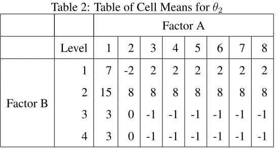
The simulation set-up consisted of a two factor design having eight levels for fac-tor A and four levels for facfac-tor B. A balanced design was used with sample sizes of 64, 192, and 320, corresponding to two, six, and ten replications per treatment combination respectively. The response was generated according to a normal distribution with an error variance of one. Two different effect vectors, θ1 andθ2 were used and the table of cell means corresponding to each vector are given in tables 1 and 2.
*****FIGURE 1 AND 2 GO HERE*****
We can see that in terms of the cell means table, aφα,ij group is zero only if column iandj are equal and aφβ,ij group is zero only if rowiandjare equal. The vectorθ1 consisted of four distinct levels with 18 true nonzero differences between levels for factor A and three distinct levels having five true nonzero differences between levels for factor B. Using the full rank baseline reparametrization, there were 68 truly nonzero pairwise differ-ences of interest and 71 truly zero pairwise differdiffer-ences of interest. The vectorθ2consisted of three distinct levels for both factors, with 13 and five true nonzero differences between levels for factor A and B, respectively. In terms of pairwise differences of interest, there were 61 truly nonzero differences and 78 truly zero differences. The analysis was run on 300 independent data sets at each setting of sample size and effect vector.
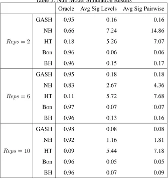
In order to inspect the control of the family-wise error rate (FWER), null model simu-lations (all true parameter vectors set to zero) were also conducted. The simulation set-up above was used with two, four, and eight replications and an error variance of 16.
6.2 Competitors and Methods of Evaluation
were evaluated at the 0.05 level. If none of the p-values in aφα,ij orφβ,ijgroup were sig-nificant then levelsiandjfor the corresponding factor were considered collapsed. If any of the p-values in a group were significant, then the corresponding levels were considered to be significantly different. Note that these methods also do not encourage the collapsing of levels the way we desire. For the GASH-ANOVA and the No Heredity methods, if all of the differences in aφα,ij orφβ,ijgroup were estimated at zero then levelsiandjof the
corresponding factor were considered collapsed. If any of the differences in a group were nonzero then the corresponding levels were considered to be significantly different.
We use the setsAα, Aα,n, Aβ,andAβ,nto define the criteria that are used for
compar-isons of the procedures. Due to the different procedures for deciding if we collapse two levels or deem them significantly different, we must extend our definitions of Aα,n and Aβ,n. DefineAα,n =
n
(i, j) :F( ˆφα,ij)6= 0o,where
F( ˆφα,ij) =
||φα,ijˆ ||2 for GASH and NH methods
1Iφˆα,ij for hypothesis testing methods
and1Iφˆα,ij is an indicator function that is one if any p-value in theφˆα,ij is deemed
signifi-cant and zero otherwise. The setAβ,nis defined similarly.
The GASH-ANOVA, NH, HT, Bon, and BH methods were all evaluated and compared on a number of criteria. Let us consider the null hypothesis that we collapse two levels of a factor against the alternative that those levels differ significantly. A ‘1-TypeI’ error criterion is defined as |A
c
α,n∩Acα|+|Acβ,n∩A c β|
|Acα|+|Aβc| ,where |A|is the cardinality of A. In words,
this is the number of collapsed level differences found that truly should have been col-lapsed divided by the true total number of colcol-lapsed level differences. A ‘Power’ criterion was likewise defined as |Aα,n∩Aα|+|Aβ,n∩Aβ|
|Aα|+|Aβ| or the number of significantly different level differences found that truly differed divided by the true total number of significantly dif-ferent level differences. The number of collapsed differences between levels in each data set (Collapsed) was found along with the false collapse rate (FCR), which is the num-ber of incorrectly collapsed differences divided by the numnum-ber of collapses found, i.e.
|Acα,n∩Aα|+|Acβ,n∩Aβ|
|Acα,n|+|Acβ,n| . The number of significant differences between levels in each data set (Sig) was also found along with the false significance rate (FSR), which is the number of incorrect significantly different level differences found divided by the total number of significantly different level differences found, i.e. |Aα,n∩A
c
α|+|Aβ,n∩Acβ|
de-fine these criteria for the pairwise differences of interest. All of the criteria were averaged across the 300 data sets. These results are given in tables 3 and 4.
Table 5 was produced from the null model simulation. This table gives the oracle per-cent. That is, the percent of datasets such thatAα =Aα,nandAβ =Aβ,n, which acts like the FWER in this situation. The average number of significant differences found between both levels and pairwise differences of interest was also reported.
6.3 Simulation Results
Looking at the ‘1-Type 1’ and ‘Power’ columns of tables 3 and 4, we see that the GASH-ANOVA procedure is the only method that has high ‘power’ for finding both the significant level differences and significant pairwise differences. This is due to the heredity-type structure that the method requires its model to have. The other methods may be able to find one or more of the pairwise differences of a truly nonzero level difference significant (leading to high level power), but the GASH-ANOVA procedure’s structural constraint forces all pairwise differences of interest for a level to be significant if the level difference is significant. Thus, we see the advantage and usefulness of the constraint. The GASH-ANOVA procedure also dominates the NH procedure in terms of the ‘1-Type 1’ cri-terion for the levels for both effect vectors and for pairwise differences for effect vectorθ2. The corrected hypothesis testing procedures perform very well in this aspect, but lack the power to find significant pairwise differences, especially compared to the GASH-ANOVA procedure.
*****FIGURE 3 AND 4 GO HERE*****
number, but the average number of significant pairwise differences found is far too small in every case.
*****FIGURE 5 GOES HERE*****
We are also interested in how each method does in terms of controlling the FWER. Table 5 shows that the corrected hypothesis testing methods do as they are designed to, hold the FWER approximately at 0.95. We can see that the NH method performs better for this criterion as the sample size grows, but the GASH-ANOVA procedure performs extremely well in all cases and that the FWER approaches one as the sample size grows. Thus, we can see that not only does the GASH-ANOVA method tend to have the best performance in terms of power, its control of the family-wise error rate is extremely good as well.
7
Real Data Example
The GASH-ANOVA procedure was applied to data from a memory trial done by Eysenck (1974). The trial was designed to investigate the memory capacity of two ages of people (Young and Old) by having them recall a categorized word list. There were 50 subjects in each age group that were randomly assigned to one of five learning groups: Counting, Rhyming, Adjective, Imagery, and Intentional. The Counting group was to count and record the number of letters in each word. The Rhyming group was told to think of and say out loud a word that rhymed with each word given. The Adjective group was to find a suitable modifying adjective for each word and to say each out loud. The Imagery group was to create an image of the word in their mind. These learning groups were increasing in the level of processing required with Counting being the lowest level and Imagery being the highest. The subjects assigned to the first four learning groups were not told they would need to recall the words given, but the Intentional group was told they would be asked to recall the words.
BH and Bonferonni p-value correction methods were applied to the data and evaluated in the same manner that was done in the simulation studies.
*****FIGURE 6 AND 7 GO HERE*****
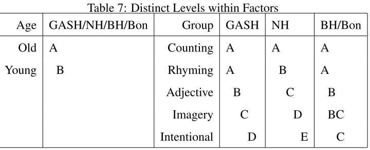
As we can see from table 6, the GASH-ANOVA solution collapsed the Counting and Rhyming treatment groups but did not collapse any other levels from either factor. The NH method did not collapse any levels of either factor. It did collapse the main effects for the Rhyming and Counting groups, but the corresponding interaction difference was estimated as nonzero. This implies that Rhyming and Counting learning groups were collapsed for the Old age group only. The BH and Bonferonni procedures found that the Counting and Rhyming groups, the Adjective and Imagery groups, and the Imagery and Intentional groups were not different. These two methods did happen to collapse the interactions corresponding to those main effects.
Here we can see that the p-value correction methods form overlapping groups. The NH method does create non-overlapping groups, however, it seems that the lack of model structure may have prevented two levels from being collapsed. The p-value correction methods do follow the level collapsing structure in this example, but this need not be the case. Based on the simulation results, the p-value correction methods also suffer from lack of power. We see this here as the GASH-ANOVA procedure is able to detect more significant differences between the levels of the learning group factor. Thus, we can see the advantages inherent in the GASH-ANOVA procedure. The GASH-ANOVA procedure’s estimates are designed to encourage the collapsing of levels and they have the advantage of automatically creating non-overlapping groups.
8
Discussion
differences of interest, and maintaining high family wise error rate, the GASH-ANOVA procedure performs the best of all the methods compared. The computation for the prob-lem is shown to be a quadratic programming probprob-lem with linear constraints and is feasible in most situations.
9
Appendix
Proof of Theorem 1:
Proof of a): LetBα,n =Aα,n∩AcαandBβ,n =Aβ,n∩Acβ be the indices of the main
effect differences for factor A and B, respectively, that should be estimated at zero but were incorrectly estimated as nonzero. We need to show that the true zeros will be set to zero with probability tending to one or, equivalently, that bothP(Bα,n 6=∅)→0andP(Bβ,n6=
∅) → 0. Then we must show thatP(Acα,n∩Aα 6=∅) → 0andP(Acβ,n∩Aβ 6= ∅) → 0,
i.e. that none of the nonzero differences are mistakenly set to zero. The second item to show will follow directly from the√n-consistency of the estimators for the differences in
AαandAβ, which will be proved in part b of the theorem.
For the first item, we show thatP(Bα,n 6=∅)→0and the proof forP(Bβ,n 6=∅)→0
is done similarly. AssumingBα,nis nonempty, there are two cases to consider: Case (i) A
pair of indices inBα,nhas its main effect difference as the maximum of its corresponding φα,ij group. Case (ii) No pair of indices in Bα,n has its main effect difference as the
maximum of its correspondingφα,ij group.
Case (i): Because we have categorical factors we can sort the levels of factor A so that
b
α1 ≤αb2 ≤...≤αab . Letmbe the largest index of any index pair inBα,n that is also the
maximum of itsφα,ij group, i.e.
m=max{j: (i, j)∈Bα,nfor somei, αj −αi =max|φα,ij|}.
Letqbe the smallest index such that the pair(q, m)∈Bα,n, soq < m. Now we
reparam-eterize to the full rank design matrix using levelqof factor A and some arbitrary level, say
b, of factor B as our baseline. Thus, we defineγ =µ+αq+βb+ (αβ)qb. We defineγkαas αk−αqfork6=q, defineγjβ asβj−βbforj 6=b, and defineγkjαβto be zero if and only if
both(αβ)kj−(αβ)kb = 0and(αβ)kj−(αβ)qj = 0fork6=q, j6=b. We create the new
full rank parameter vector,γ by stackingγ, theγα, theγβ, and the γαβ. By assumption
such that the main effect difference corresponding to(k, m)is the maximum of itsφα,km
group. Due to the ordering of the levels chosen, fork < lat the GASH-ANOVA solution we have
|αl−αk|=
γαl −γkα k6=q, l6=q
γα
l k=q, l > q
−γkα k < q, l=q
Hence, we can rewrite the solution as
b
γ=argminγ
h
||y−Zγ||2+λnJ(γ)
i
, (4)
where
J(γ) =
P
1≤k<q−1
w√(αkq)
n max
n
(−γkα,
Γ αβ k+ )
To+
P
q<k≤a w√(αqk)
n max
n
(γkα,
Γ αβ k+ )
To+
P
1≤k<l≤a,k6=q,l6=q w√(αlk)
n max
n
((γlα−γkα),
Γ
αβ l+,k+
)
To+
P
1≤k<b−1
wβ(kb)
√ n max n ( γ β k , Γ αβ +k )
To+
P
1≤k<l≤b−1
w(βkl)
√ n max n ( γ β l −γ
β k , Γ αβ
+l,+k
) To , (5)
Z is the typical design matrix for the parametrization that treats levelq of factor A and levelbof factor B as the baseline and
Γ αβ k+ = ( γ αβ k1 , γ αβ k2 , ..., γ αβ k(b−1)
), Γ αβ l+,k+
= ( γ αβ l1 −γ
αβ k1 , γ αβ l2 −γ
αβ k2 , ..., γ αβ l(b−1)−γ
αβ k(b−1)
), Γ αβ +k = ( γ αβ 1k , γ αβ 2k , ..., γ αβ
(a−1)k
), Γ αβ
+l,+k
= ( γ αβ
1l −γ αβ 1k , γ αβ
2l −γ αβ 2k , ..., γ αβ
(a−1)l−γ αβ
(a−1)k
).
To complete this part of the proof we will obtain a contradiction on a neighborhood of our solutionbγm. At the solution the optimization criterion above is differentiable with
respect toγmα becausebγmα 6= 0. We investigate this derivative on a neighborhood of the solution on which the differences that are estimated at zero remain at zero. On this neigh-borhood, the terms involving(k, m) ∈ Acα,n∩Acα can be omitted since they will vanish in the objective function. Because our criterion is differentiable on the neighborhood, our solutionγbmust satisfy
2 √
nz T
m(y−Zγb) = λn √ n P
k6=m,(k,m)∈Aα(−1)
I[m<k]w√(αkm)
n I[bγ
α m]
+√λn
n
P
k6=m,(k,m)∈Bα,n
wα√(km)
n I[bγ
wherezmT denotes themthcolumn ofZ andI[bγ
α
m]is an indicator that is one if the
maxi-mum of|φα,km|was a main effect and zero otherwise.
By construction, all of the terms in the second sum on the right hand side are pos-itive and, for this case, the second sum is nonempty. Note that for all (k, m) ∈ Bα,n
we have w(αkm) = |αm,OLSb −αk,OLSb |
−1
. Also for any (k, m) ∈ Aα the weight is of
the form w(αkm) = |αbm,OLS−αbk,OLS|
−1 or w(km)
α =
([αβ)ml,OLS−([αβ)kl,OLS
−1 where l is some level of factor B. Therefore, for all ksuch that (k, m) ∈ Aα we have w(αkm) =Op(1), while for(k, m) ∈Acα, n−1/2w
(km)
α =Op(1)since the initial OLS
esti-mator is√n-consistent. Thus, the first sum on the right hand side isOp(λnn−1/2)and the
terms in the second sum areOp(λn). Since the second sum is nonempty, the entire right hand side must beOp(λn)since at least one term must be.
However, the left hand side isOp(1)and by assumptionλn→ ∞. This is a contradic-tion, thus it must be thatP(Bα,n 6=∅)→0.
Case (ii)The proof proceeds much like that for case (i). Find the pair(m, q)such that for allj = 1,2, ..., b,([αβ)
mj −([αβ)qj is the largest estimated difference of any pair in
Bα,n. Thus,
([αβ)mj−([αβ)qj
is also the maximum of its corresponding φα,ij group.
Without loss of generality sort the levels of factor A so that([αβ)
1j ≤ ([αβ)2j ≤ ... ≤ [
(αβ)aj, letq < m, and assumej6=b. As with case (i), we reparameterize to the full rank design matrix using levelqof factor A and levelbof factor B and form the new parameter vectorγ. Thus,(αβ)mj−(αβ)qj = 0only ifγmjαβ = 0andbγ
αβ
mjis positive and nonzero.
We will find a contradiction by taking the derivative of the full rank optimization crite-rion with respect toγmjαβ on a neighborhood of the solution where the differences that are estimated at zero remain at zero. We can rewrite the optimization criterion with terms in the penalty not involvingγαβmjomitted as follows:
b
γ =argminγ
h
||y−Zγ||2+λn(Q1(γ) +...+Q6(γ))
i
, (7)
whereQ1(γ), ..., Q6(γ)are given by
w√(αkq) n max
n
(|γmα|,
γ αβ m1 , ..., γ αβ mj , ..., γ αβ m,b−1
)
To,
X
1≤k<q−1
w(αmk)
√
n max
n
(|γmα −γkα|,
γ
αβ m1−γ
αβ k1 , ..., γ αβ mj −γ
αβ kj , ..., γ αβ m,b−1−γ
αβ k,b−1
)
To,
X
q+1<k≤a w√(αmk)
n max
n
(|γkα−γmα|,
γ
αβ k1 −γ
αβ m1 , ..., γ αβ kj −γ
αβ mj , ..., γ αβ k,b−1−γ
αβ m,b−1
)
w(βjb) √ n max n ( γ β j , γ αβ 1j , ..., γ αβ mj , ..., γ αβ aj )
To,
X
1≤k<j wβ(jk)
√ n max n ( γ β j −γ
β k , γ αβ
1j −γ αβ 1k , ..., γ αβ mj−γ
αβ mk , ..., γ αβ aj −γ
αβ ak
)
To,
and
X
j<k<b w(βjk)
√ n max n ( γ β k −γ
β j , γ αβ
1k −γ αβ 1j , ..., γ αβ mk−γ
αβ mj , ..., γ αβ ak −γ
αβ aj
)
To,
respectively. Note that by choice of the baseline, the interaction parameters in the groups corresponding to factor B do not contain any parameters whereqis the first index (i.e.γαβqj
does not appear in the groups for allj). At the GASH-ANOVA solution we have
γ αβ mj = γ αβ
mj and we know thatγ αβ mj is the
maximum of its correspondingφα,mj group (the first group above). For the other groups in the penalty that correspond to factor A, if the term with γmjαβ is the maximum of the group we have that for allk < qork > m,(m, k) ∈/ Bα,n, else a difference larger than [
(αβ)mj−([αβ)
qjcould be found and for allq < k < m,
γ
αβ mj−γ
αβ kj =γ αβ mj−γ
αβ kj. Note
thatγmjαβ ≥
γ αβ mk
for allk, k = 1,2, ..., b−1. Thus, for the groups in the penalty that
involve differences ofγmjαβ corresponding to factor B, if that difference is the maximum of the group we have that
γ
αβ mj −γ
αβ mk = (γ αβ mj−γ
αβ mk)or(γ
αβ mj+γ
αβ mk).
On the neighborhood described we can differentiate our criterion to get an equation similar to equation 6. In doing so we can use a similar argument as used in case (i) to show our contradiction. The sums that involved indices inBα,n consist of only positive values,
are nonempty, and are of orderOp(λn). Likewise, indices inBβ,nconsist only of positive
values and are of orderOp(λn). All other terms on the right hand side of the equation are
Op(λnn−1/2) implying the right hand side must be of order Op(λn). However, the left
hand side isOp(1)and by assumption λn → ∞. This again is our contradiction, thus it must be thatP(Bα,n 6=∅)→0.
Proof of b): As with the proof of the CAS-ANOVA asymptotic normality, this proof will closely follow that of Zou (2006). The proof given below is just a sketch of how the proof is adapted to this setting, for full details please see Zou (2006). Letγ0 be the true parameter vector for the full rank reparametrization and letuˆ =√n(γb−γ0).Now, ˆ
u=arg minuVn(u), where
Vn(u) =uT(
1
nZ
TZ)u−2√TZ nu+
λn
√
and
P(u) =
X
k6=q
(−1)I[k<q]w (kq)
α √ n √ nmax ((
γkα0+√uk
n
− |γkα0|),(
Γαβkj0+√ukj
n − Γ αβ kj0 )) T + X 1≤k<l≤a,k6=q,l6=q
w√α(kl) n √ nmax ( γ α
l0−γkα0+
ul√−uk
n
− |γ
α
l0−γkα0|,
Γ
αβ lj0,kj0+
ulj0√−ukj0
n − Γ αβ lj0,kj0
) T + X 1≤j<b−1
wβ(jb)
√ n √ nmax (
γjβ0+√uj
n − γ β j0 ,
Γαβij0+√uij
n
− |Γij0|)T
+ X 1≤j<m≤b−1
wβ(jm)
√ n √ nmax ( γ β l0−γ
β j0+
ul√−uj
n , Γ αβ im0,ij0+
uim√0−uij0
n
− |Γim0,ij0|)
T
.
By the argument in Zou (2006), √λn
nP(u)will go to zero for the correct model structure
and diverge under the incorrect model structure. LetVnO(uO)be the value of the objective
function obtained using the ‘oracle’ structure determined byAαandAβ. This implies we
collapseZtoZOby combining the columns of the columns of each pair inAcαandAcβ, in
the process forming a newγO. IfηbAcα,Acβ = 0, thenVn(u) =V
O n (uO).
Assuming constant variance, σ2, for our model we get 1nZOTZO → C,where C is a
positive definite matrix. Also we have that T√ZO
n → W =N(0, σ
2C). As in Zou (2006),
we getVn(u)→V(u), where
V(u) =
uT
OCuO−2uTOW ηbAcα,Acα = 0
∞ otherwise
.
SinceVn(u)is convex and the unique minimizer ofV(u)is(C−1W,0)T, the asymptotic
normality follows. Therefore,uTAα,A
β → N(0, σ
2C−1). The result for all pairwise differ-ences,ηbAα,Aβ, follows after the (singular) transformation.
References
Benjamini, Y. and Hochberg, Y. (1995). Controlling the false discovery rate: A practical and powerful approach to multiple testing. Journal of the Royal Statistical Society B, 57:289–300.
Bondell, H. D. and Reich, B. J. (2009). Simultaneous factor selection and collapsing levels in ANOVA. Biometrics, 65:169–177.
Chipman, H. (1996). Bayesian variable selection with related predictors. The Canadian Journal of Statistics, 24:17–36.
Choi, N., Li,W. and Zhu, J. (2010). Variable selection with the strong heredity constraint and its oracle property. Journal of the American Statistical Association, 105:354–364.
Fan, J. and Li, R. (2001). Variable selection via nonconcave penalized likelihood and its oracle properties. Journal of the American Statistical Association, 96:1348–1360.
Franck, C., Osborne, J., and Nielsen, D. (2011). An all congurations approach for detecting hidden-additivity in two-way unreplicated experiments.North Carolina State University Technical Report.
Hamada, M. and Wu, C. (1992). Analysis of designed experiments with complex aliasing.
Journal of Quality Technology, 24:130–137.
Tibshirani, R. (1996). Regression shrinkage and selection via the lasso. Journal of the Royal Statistical Society B, 58(1):267–288.
Yuan, M., Joseph, V. and Lin, Y. (2007). An efficient variable selection approach for analyzing designed experiments. Technometrics, 49:430.
Yuan, M., Joseph, V. and Zou, H. (2009). Structured variable selection and estimation.
The Annals of Applied Statistics, 3:1738–1757.
Zhang, P., Rocha, G. and Yu, B. (2009). The composite absolute penalties family for grouped and hierarchical variable selection. The Annals of Statistics, 37:3468–3497.
Zou, H. (2006). The adaptive lasso and its oracle properties. Journal of the American Statistical Association, 101(476):1418–1429.
Zou, H. and Hastie, T. (2005). Regularization and variable selection via the elastic net.
Journal of the Royal Statistical Society B, 67(Part 2):301–320.
Table 1: Table of Cell Means forθ1 Factor A
Level 1 2 3 4 5 6 7 8
Factor B
1 2 4.5 -1 0 2 2 2 2
2 4.5 8.5 2.5 3 4.5 4.5 4.5 4.5
3 3 5 2 0 3 3 3 3
4 3 5 2 0 3 3 3 3
Table 2: Table of Cell Means forθ2 Factor A
Level 1 2 3 4 5 6 7 8
Factor B
1 7 -2 2 2 2 2 2 2
2 15 8 8 8 8 8 8 8
3 3 0 -1 -1 -1 -1 -1 -1
Table 5: Null Model Simulation Results
Oracle Avg Sig Levels Avg Sig Pairwise
Reps= 2
GASH 0.95 0.16 0.16
NH 0.66 7.24 14.86
HT 0.18 5.26 7.07
Bon 0.96 0.06 0.06
BH 0.96 0.15 0.17
Reps= 6
GASH 0.95 0.18 0.18
NH 0.83 2.67 4.36
HT 0.11 5.72 7.68
Bon 0.97 0.07 0.07
BH 0.96 0.13 0.16
Reps= 10
GASH 0.98 0.08 0.08
NH 0.92 1.16 1.81
HT 0.09 5.44 7.18
Bon 0.96 0.05 0.05
Table 6: Treatment Combination Means and Distinct Levels
Age Group Mean SD GASH NH BH/Bon
Young Counting 6.5 1.43 A A A
Young Rhyming 7.6 1.96 A B A
Young Adjective 14.8 3.49 B C B
Young Imagery 17.6 2.59 C D BC
Young Intentional 19.3 2.67 D E C
Old Counting 7.0 1.83 E F D
Old Rhyming 6.9 2.13 E F D
Old Adjective 11.0 2.49 F G E
Old Imagery 13.4 4.50 G H EF
Old Intentional 12.0 3.74 H I F
Table 7: Distinct Levels within Factors
Age GASH/NH/BH/Bon Group GASH NH BH/Bon
Old A Counting A A A
Young B Rhyming A B A
Adjective B C B
Imagery C D BC