Electronic Theses and Dissertations Theses, Dissertations, and Major Papers
1-1-1981
Heuristic approaches to quadratic assignment problems.
Heuristic approaches to quadratic assignment problems.
Suresh Chandra Jaisingh
University of Windsor
Follow this and additional works at: https://scholar.uwindsor.ca/etd
Recommended Citation Recommended Citation
Jaisingh, Suresh Chandra, "Heuristic approaches to quadratic assignment problems." (1981). Electronic Theses and Dissertations. 6123.
https://scholar.uwindsor.ca/etd/6123
b y
Suresh Chandra Jaisingh
A Dissertation
Submitted to the Facu l t y of Graduate Studies
through the Dep a r t m e n t of
I ndustrial E n g i n e e r i n g in partial fulfillment
of the requirements for the Degree
o f D o c t o r of Phi l o s o p h y at
The U n i v e r s i t y of Windsor.
Windsor, Ontario, Canada.
INFO RM ATIO N TO USERS
The quality of this reproduction is dependent upon the quality of the copy
submitted. Broken or indistinct print, colored or poor quality illustrations
and photographs, print bleed-through, substandard margins, and improper
alignment can adversely affect reproduction.
In the unlikely event that the author did not send a complete manuscript
and there are missing pages, these will be noted. Also, if unauthorized
copyright material had to be removed, a note will indicate the deletion.
UMI
UMI Microform D C 5 3 2 1 6 Copyright 2009 by ProQuest LLC
All rights reserved. This microform edition is protected against unauthorized copying under Title 17, United States Code.
ProQuest LLC
789 East Eisenhower Parkway P.O. Box 1346
)
9?!
Z51
This study is directed towards the development of heuristic
algorithms for the solution to the quadratic assignment problem. This
is the problem of minimizing the 'cost' of assigning n 'facilities'
to n given 'sites', when there is an interflow. The combinatorial
nature of the problem indicates that for a problem of size n, there
are n! possible assignment vectors. Since it is computationally
infeasible to generate all the possible assignment vectors for n ^ 12,
heuristic procedures are developed which generate only a subset of
them.
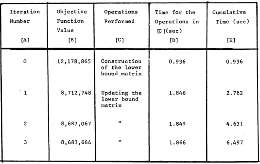
The algorithm developed in this study is an iterative
optimization procedure which begins by constructing the matrix of
lower bounds on the 'costs' of locating facilities at different sites.
Any feasible assignment vector may or may not have cfptimum values
associated with its components in this matrix. Thus, the algorithm
seeks to remove the deviations from the optimum values in the elements of
the lower bound matrix. After all the elements in the matrix have been
adjusted, a linear assignment problem is solved, which results
in a feasible assignment vector as well as an improved objective function
value for the quadratic assignment problem. The procedure is repeated
until the desired accuracy in the value of the objective function is
few iterations. It then decreases in subsequent iterations. Further,
the proposed algorithm ,is independent of starting solution.
Finally, sensitivity analysis is carried out to study the
effect of varying the parameters in the distance or flow mat r i x on
the layout. No obvious pattern is observed. However, it is concluded
that , to reduce the computational efforts, the information contained
in the final iteration of the original problem could be used to study
the effects of the changed parameter on the layout. Reapplying the
Dissertation advisor, Dr. R.S. Lashkari, for providing direction and
encouragement to m y Ph.D. program and to this research. His
accessibility and his willingness to discuss any of the difficulties
encountered is specially appreciated.
Special thanks are extended to Dr. K.G. Murty of the University
of Michigan for serving as the external examiner to the dissertation
committee.
Also the author wishes to express thanks to other members of the
Dissertation Advisory Committee for stimulating and evaluating ideas.
These members are: Dr. A. Raouf, Professor of Industrial Engineering,
Professor A.A. Danish, Associate Professor of Industrial Engineering,
Dr. M. Shridhar, Professor of Electrical Engineering and Dr. R. Barron,
i l l
ABSTRACT
ACKNOWLEDGEMENTS vi
LIST OF TABLES %
LIST OF FIGURES x i
CHAPTER I. INTRODUCTION 1
1.1 Classification of Facilities Location Problems 2 (i) Quadratic Assignment Problem (QAP) 2 (ii) Linear Assignment Problem (LAP) 3
1.2 Applications 4
(i) Plant Layout Problem 4
(ii) Travelling Salesman Problem 6
(iii) Rotor Balancing Problem 7
II. SURVEY OF EXISTING METHODS OF SOLUTION 8
2.1 Exact Solution Procedures 8
(i) Solutions Based on Integer Programming 9 (ii) Solutions Based on Branch and Bound 12 (a) Single Assignment Algorithm 13 (b) Pair-Assignment Algorithm 19 (c) Pair Exclusion Algorithm 21
2.2 Heuristic Solution Procedures 24
(i) Construction Methods 24
(ii) Improvement Methods 28
(iii) Algebraic Methods 22
(iv) Stochastic Methods 24
2.3 Computational Experiences and the Comparative Studies 25
2.4 Motivation 29
III. DEFINITION OF PROBLEM AND OUTLINE OF SOLUTION METHODOLOGY 45
3.1 Introduction 45
3.2 Formulation of the Problem 45
4.3 The Least-Allocation Cost Criterion 57
4.4 The Pseudo-Random Assignment Criterion 58
V. FACTORS INFLUENCING THE SOLUTION EFFICIENCY 59
5.1 Introduction 59
5.2 Linear Assignment Problem (LAP) 60
5.3 Determination of Several Solutions to LAP 60 Simultaneously
VI. SUMMARY OF SOLUTION PROCEDURE 65
6.1 Introduction 65
6.2 The Algorithm 66
6.3 Stopping Criteria 70
VII. DISCUSSION OF RESULTS 72
7.1 Introduction 72
7.2 Application of Algorithm to Test Problems 72 (i) Test Problems Suggested by Nugent, et al. 72
[1968]
(ii) Practical Problem Suggested b y Elshafei 76 [1977]
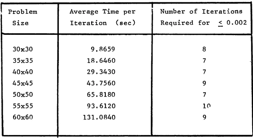
(iii)Randomly Generated Large Problems 79
7.3 Sensitivity Analysis 87
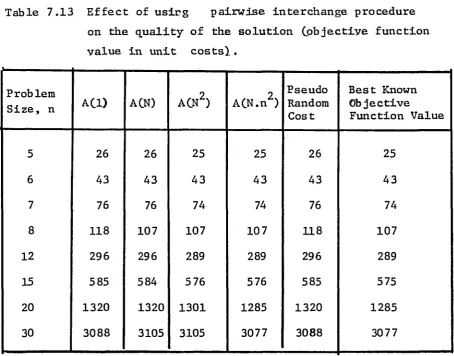
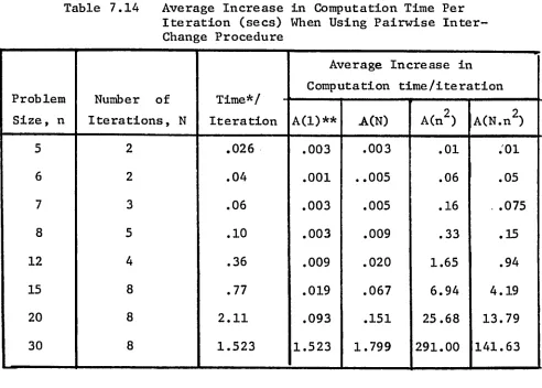
7.4 Effects of Using Pairwise Interchange Procedure 109 In Conjunction with the Algorithm
VIII. CONCLUSIONS AND RECOMMENDATIONS 114
APPENDICES
I A Method for Finding Several Solutions to the Assignment Problem Simultaneously.
117
II Data for the Test Problems 136
III Data for the Practical Problem 150
IV Computer Program 152
REFERENCES 180
2.1 Summary of Comparative Results of Various Heuristic 40 Procedures
2.2 Summary of Computational Times Per Solution For 41 Various Heuristic Procedures
7.1 Results of Different Heuristic Procedures 74
7.2 Summary of Computation Times Per Solution 75
7.3 Summary of Results of Pratical Problem, Given by 78 Elshafei [1977]
7.4 Summary of Computational Experiences on Large Size Problems
7.5 Results of Ran d o m Generation of Problem Size 4x4
7.6 Results of Random Generation of P r o blem Size 5x5
7.7 Results of Ran d o m Generation of P r o blem Size 6x6
7.8 Data for Sample P r o b l e m of Size 10x10 for Sensitivity 90 Analysis
7.9 Effect of Varying the Parameter in a Problem of 92 Size 10x10
7.10 Effect of Varying the Parameter d._ in a P r o blem of 98
Size 10x10 10
7.11 Data for a Sample Problem of Size 20x20 for Sensitivity 2-00 Analysis
7.12 Effect of Varying the Parameter d., _ in a P r o blem of 2-04
Size 20x20 i'^
7.13 Effect' of Using Pairwise Interchange Procedure on the 2.12 Quality of the Solution
Figure No. Title Page
2.1 Search Tree With Each Level Representing A 15 Unique Plant
2.2 Search Tree With Each Level Representing A 18 Unique Location
2.3 Tree Diagram For Pair Exclusion Algorithm 23
2.4 Improvement Algorithms Based On Interchange 31 Procedure
7.1 Increase in Average Time per Iteration vs. Problem 82 Size
7.2 Improvement in the Quality of the Solution vs. 83 Iteration Number
7.3 Effect of Varying the Parameter w.. « on Layout When 91 Reapplying The Algorithm in a Problem of Size 10x10
7.4 Effect of Varying the Parameter on Layout When 92 Using the Previous Information in a Problem of Size
10x10
7.5 Effect of Varying the Parameter d _ _ on Layout When 96 Reapplying the Algorithm in a Problem of Size 10x10
7.6 Effect of Varying the Parameter d^g on Layout When 97 Using Previous Information in a Problem of Size 10x10
7.7 Effect of Varying the Parameter d _ on Layout Wh e n 102 Reapplying the Algorithm in a Problem of Size 20x20
7.8 Effect of Varying the Parameter d^^ on Layout When 103 Using the Previous Information in a Problem of Size
Facilities location problems have been the subject of analysis
for many years. However, it was not until the emergence of interest
in operations research that the subject received renewed attention
in a number of disciplines. During the recent years, economists,
operations researchers, urban planners, management scientists, home
economists, and engineers from several disciplines, have discovered
a common interest in their concern for the location and layout of
facilities. Each group has attempted to bring to the subject
different interpretations of the problem and different approaches to
its solution. The industrial engineers find it useful in laying out
activities, offices, or departments in a building, etc.
There is a multitude of problems within facilities location. Of
these we shall restrict our attention to those problems which are of
a general nature. "Facilities location" shall now be designated as
problems involving the assignment of n distinct facilities to n^
distinct locations (n < n, ), when there is a cost function to be — 1
minimized. The facilities location problems which are of special
The general QAP can be stated as follows. Given n^ coefficients
c. . . the problem is to find an nxn permutation matrix
ijpq ijpq
X = [ X ..1 so as to minimize ij
y y c . . X . . X (1 .1 )
ij pq "2 M
This was first formulated in location context by Koopmans and
Beckmann [1957]. It can also be stated as the determination of nxn
permutation matrix X = [x\j] so as to minimize
f(x) = y a.. X.. + y y f. d. x . . x (1 .2 )
ij
"J ij pq 2q ip 1] pq
where A - [a..], F = [f. ] and D = [d. ] are nxn matrices,
ij jq ip
representing the following parameters :
a^j = fixed cost associated with the location of facility j at
location i
f. = the number of units of commodity to be transported from
jq
facility j to facility q
d^p = the cost of transporting one unit of commodity from location
i to location p
= 0 otherwise
This formulation is of great interest and provides the basic
framework for a wide class of problems.
It is interesting to note that if f^^ = 0, for all (j,q).
Equation (1.2) represents a linear assignment problem, which is
employed in various algorithms for QAP, and which is formulated
in the following section.
(ii) Linear Assignment Problem (LAP)
Consider n facilities to be located, one at each location and
assume that there are exactly n locations available. Let x . . be the ij
variable defined in l.l(i). Thus
x^j = 0 or 1 for i = l,..,n and j = l,..,n
n
y X . . = 1 for i = 1 ,.. ,n j=l
The last condition states that exactly one facility is located
at each location i. Likewise, each facility j must be located at
exactly one location, which leads to the condition:
n
y X .. = 1 for j = 1,.. ,n
n n
Minimize f(X) = 7 7 c.. x.. (1.3)
i=l j=l "2 xj
Subject to
n
I X - . = 1, j = 1 , . . ,n i=l
n
i = l,..,n ) (1.4)
= 0 or 1 for all i and j
1.2 Applications
(i) Plant Layout P r o blem [Koopmans & Beckmann, 1957]
This is the problem of locating n plants uniquely at n locations
in such a way that the total interplant transportation cost is
minimized. In the context of the formulation given in (1.2), the
variables can be defined as:
= fixed cost associated with the location of plant j at location i
fjq - the number of units of commodity to be transported from plant
q to plant j
= the cost of transporting one unit of commodity from location p
x^j = 1 if location i is assigned to plant j
= 0 otherwise
This formulation is often employed in (i) placement of
electronic modules on a computer backplane so as to minimize wire
length; number of crossings, etc. [Hanan and Kurtzberg, 1972] ;
(ii) locating machines, departments, or offices within a plant so
as to minimize transportation efforts [ Armour and Buffa, 19631 ;
(iii) arranging indicators and controls in a control room so as to
minimize eye fatigue [McCormick, 1970 ]; (iv) laying out offices in
building, or operating rooms in hospitals with the monetary
objective of reducing the cost of office accomodation [ Whitehead and
Elders, 1964] , and relocating civil service departments with the
social objective of providing employment in developing areas [ Beale
and Tomline, 1972 ] ; (v) locating hospital departments so as to
minimize the total distance travelled by the patients [ Elshafei,
1977 ]; and (vi) assigning n people to serve on m committees,
(committee/coworker performance problem) [Maybee, 1978] .
As a generalization to this formulation, Lawler [ 1963 ] discussed
the multicommodity version, in which there is a flow f^^ for each
assignments. Combining these two, Pierce and Crowston [1971]gave a
more general cost function as
M i n i m a f(x) = J, a. . X. . 4- w. x. . x^^ + I 4 p ='ij ==pq
where
w. . + xjpq
Xjpq (cz. + f .. d .. xj 2 2 11
I fjq d.p if i 5^ P or j q
if i = P and j = q
(ii) Travelling Salesman Problem
The'Travelling Salesman Problem' is a special case of the Koopmans
and Beckmann formulation in which d^^ represents the distance between
the pairs of cities and f r e p r e s e n t s the cyclic permutation matrix
of the form:
T =
0
0
0
1
1
0
0
0
0
1
0
0
This formulation is used in solving the 'Candidates P r o b l e m '.
This is the problem of finding optimum tours for the candidates in such
in such a way that the static balance is achieved relative to two
orthogonal axes. It is assumed that n mounting positions are equidistant
around the circumference of a circular rim of radius r. Let m^ designate
the distance from the centre of gravity to the mounting end of blade i,
and designate the blade's weight. If the mounting positions are
numbered counter-clockwise from one of the axes, the orthogonal components
of the moment arm W^(r + m^) produced by mounting blade i in position
i can be expressed as:
^ij " (r + m^) cos (2*j/n)
and,
= W\ (r + m^) sin (2nj/n).
If it is desired to assign blades to positions in such a way that
the sum of the moment components are both as close to zero as possible,
the equivalent QAP as formulated by Maybee [1978] can be expressed as
the determination of the permutation matrix X = [x^^] so as to
minimize f(x) = 7 7 ( h . . h + V . . V ) x . . x ij pq XJ pq XJ pq ij pq
which is of the form of general QAP if
Over the years a number of solution procedures have been
developed. In asmuch as a systematic evaluation of these procedures
is not available, it is the purpose of this chapter to provide a
general classification scheme, and to present a brief survey of the
important exact and heuristic algorithms that exist to date.
2.1 Exact Solution Procedures
Exact solutions can be sought in several ways. One w a y is to
enumerate all the assignments, and choose the one with the minimum
cost. Since the number of assignments is n ! , it is practical to do
so for small size problems. However, difficulties arise for
moderate and large values of n. The first mathematical
approach in the direction of developing an exact solution is given
by Wimmert [1958] . He presented a method based on ranking the cost
matrix and choosing coordinates close to the diagonal. However,
Conway and Maxwell [1961] gave a counter example to invalidate Wimmert*s
model. The exact solution procedures developed so far can be grouped
formulated by La w l e r [1963]. If n varia b l e s x . . are linearized XJ
by def i n i n g n varia b l e s as
y .. = X. . X
xjpq ij pq
The equivalent linear p r o g r a m can be stated as
M i n i m i z e ) c .. y . .
ijpq ijpq ijpq
Subject to y X . . = 1 (i = l,2,..,n) j
J X , , - 1 (j = 1 , 2 , . . ,n) XJ
‘ij ^pq " Zyjjpq - ° (x.i.P.q. = 1 ,2 , ..,n)
= 0 or 1 (i,j = 1 ,2 ,..,n)
^i jpq = 0 2 ( x , j , P , q = 1 , 2 , ..,n)
The proof of the e q uivalence of the two problems can be referred
to in Lawler [1963]. No computational experience is k nown to be
available for this approach.
Love and Wo n g [1976] gave the b i n a r y m i x e d integer progr a m m i n g
n -1 n
A . . + B . . )
XJ XJ
II X II
M i n i m i z e J 7 W . . ( R , . + L.. + i=l j=i+l "2 "2
Subject to R .. - L .. = X. - X. , i = l,..,n-l
XJ XJ 1 J )
- Bij =
i
i
=
n
X; + y; '
= I
s. a, i = 1 ,.. ,nn
*i - ?! “ J j Pk “ ik i = l....n
n
y a. = 1 i = 1 ,.. ,n
k=l
n
I ct. = 1 k = l,..,n
i=l
cc^j^ = 0 or 1 i,k = l,..,n
*ij' ^ij' *ij' Bij' y i i ' - ' P n - °
where:
n = number of facilities and num b e r of locations
w^j = non- n e g a t i v e flow b e t w e e n facility i and facility j
hij = hor i z o n t a l distance b e t w e e n facility i and facility j if
facility i is to the right of facility j; otherwise h^^ = 0
= hor i z o n t a l distance b e t w e e n facility i and facility j if
facility i is to the left of facility j ; otherwise = 0
j = vertical distance b e t w e e n facility i and facility j if
= v e rtical distance b e t w e e n facility i and facility j if
facility i is b e l o w facility j; otherwise B^j = 0
^ ^ i ’^i^~ location of facility i, i = l,..,n
s^ = sum of coordinates of location k, k = l,..,n
= difference of coordinates of location k, value of the
first coordinate m i n u s v a lue of the second coordinate.
The computational results b ased on this approach reveal that
only small size problems involving up to 8 or 9 facilities can be
solved. It is concluded that the prospects of integer programming
approach are not v e r y promising until efficient integer programming
codes are developed.
B a z a r r a and Sherali [19 80] formulated the QAP as a m i x e d integer
linear p r o g r a m by introducing a n u m b e r of n e w variables and constraints.
The p r o b l e m is defined as the m i n i m i z a t i o n of the function
m -1 m m m
i=l j“ l k=i+l 1=1 ^ijkl
Subject to
m m i = l , . . ,m-l
k - 1 m k = 2 , . . , m
3=1
m
y X . . = 1 j = l , ••,m
i=l ^2
x^j binary i,j=l,..,m
y. .... 2 1 i = l ,.. ,m-l ; k = i + l ,.. ,m
^2 jfl
2 2 2
The above problem has m integer and m (m-1) /2 continuous
2 ^ 2 4 .
variables, and 2m linear constraints, as opposed to (m +m integer
variables and m^+2m+l constraints in Lawler's formulation. This
problem can further be decomposed into a linear integer master problem
2
in m zero-one variables, and a linear subproblem and iterated between
these two problems until a suitable termination criterion is met in a
finite number of steps.
Their computational experience reveals that the procedure required
close to ml cuts in order to verify optimality, even when the starting
solution was optimal. It was therefore suggested to operate the
procedure as a heuristic b y terminating it prematurely. Its
applicability as a heuristic procedure was demonstrated with the help
of test problems given by Nugent^ et al. [1968].
(ii) Solutions Based on Branch and Bound
The idea of branch and bound dates back to the algorithm of Little,
The "branch" term represents that the procedure is continually
concerned with choosing the next feasible branch of the tree to
elaborate and evaluate, while the "bound" term indicates their
emphasis on the effective use of bounding the value of the objective
function at each node in the tree, both for eliminating dominated
paths and for selecting a next branch for evaluation and elaboration.
These procedures possess the following three important attributes
according to Pierce & Crowston [1971]:
1) Termination at any usable solution prior to the ultimate
completion of the problem solving process.
2) Exploiting in an efficient manner the information that is
available beforehand pertaining to the value of an optimal
solution. For instance, when feasible solution is known from
past experience or has been derived with the aid of a heuristic
procedure, it is used to discard the solutions having higher
costs. Thus, prior knowledge of upper or lower bounds reduces
the region that need to be searched.
3) With slight modifications, these algorithms can be employed to
find all the optimal or most preferred solutions.
The branch and bound methods developed for solving the QAP have
been classified as follows:
a) Single Assignment Algorithm. This approach was first used by
a lgorithm for solving a Koopmans and Beckmann type QAP. Their
approach employed a search strategy w h ich elaborates the tree shown
in Figure 2.1 from left to right. The ordering of the location is
taken arbitrarily or wi t h some heuristic ordering rule such as
decreasing sums 7 (d..+d. ). At each level the node is chosen,
jq
for elaboration to the next level, based on the least lower bound
among the nodes not yet elaborated. These lower bounds are obtained
by solving linear assignment problems. The process of selecting a
node in a tree continues level by level, or until a node is reached
at the level n or else lower bound exceeds the current upper bound,
and the tree evaluation process backtracks to the lowest node on the
path for which all branches have not been elaborated. The process
then selects the next node and the procedure is repeated; wh e n all
the branches have been enumerated, the p r o blem solving is complete.
Thus, it is seen that the bounding operation at each node is the
key to the algorithm. Mathematically, this can be described by
considering the objective function of the QAP:
'
h I
'ijpq "U
since X is a permutation matrix, we have
^ij *iq ^ ° if j ^ 9
and X. . X = 0 if i p
m
CM
m
CM
CM
§
I
D <
C
w w
o.
K
0) OJ p H
P
TO TO
V3
TO
P
3
00
TO
The above objective function may now be w r i tten as
f(x) . X.. (c... . + Gijpq Xpq) p i. q j
Now, define an nxn m a t r i x [buj] in which each element represents
the optimal value of LAP whose objective function is
m i n i m i z e b.^ ' =ijii ^ ^ijp, ’=pq P î* i. q î“ J
Thus for given values of i and j , b^j represents a lower bound on
the sum of n cost terms from the cost matrix. Now, if we solve the
LAP:
minimize f(x) " 7 b.. x.., ij
the solution to this p r o blem w o u l d represent a lower bound on the
2
sum of n cost terms and therefore a lower bound for any feasible
solution to the QAP.
If the lower bound is the same as the objective function value of
the QAP, the optimal solution is the solution to the LAP. Otherwise
the branch and bound procedure starts by finding lower bounds at each
node. The method of finding the lower bound is essentially the
same as discussed above. The only difference is that the elements of
the lower bound cost m a t r i x are composed of the linear cost contributions
of the fixed variables of the node in addition to the lower bound
procedure the reader is referred to Cabot and Francis [1978].
Pierce and Crowston have also suggested several alternative ways
of branching and bounding. For example, in Fig. 2.1 the plants and
locations m a y be interchanged to obtain the tree as shown in Fig.
2.2. This arrangement would give rise to the elaboration of
different partial trees of solutions with quite differing number of
nodes. Thus the time required to elaborate and evaluate a single
node in a tree can differ markedly. They further suggest that the
lower bound for the Koopmans and Beckmann formulation can be obtained
b y simply sequencing the relevant flow and distance values and forming
the inner product. For finding bounds at intermediate nodes several
methods are similarly suggested. Each of them would lead to the
elaboration and evaluation of different branches of the tree. It is
therefore stated that the relative efficiency m a y be highly dependent
on the particular form of the QAP being solved.
Burkard [1973] presented a branch and bound algorithm for the
general QAP. The lower bound cost ma t r i x is first formed. As in
Lawler's approach, an LAP is then solved on this m a t r i x to establish
an initial lower bound. The lower bounds at intermediate nodes are
obtained b y augmenting the lower bound m a t r i x to include the linear
cost contributions of the fixed variables of a node. Only one LAP is
solved to develop a lower bound for an intermediate node. This
m
m
o
0
1
s
Q U
o
1-1 0) 3 D*
I
c
0) (0 0) w CL
>
u
(9 M
0) 0) u H
kl (d <u
CO
y 60
0)
>
at intermediate nodes. The superiority of this procedure over
Lawler's may be due to significant differences in computational
requirements for finding the lower bounds at each node.
Maybee [1978] developed an efficient branch and bound technique
based on the iterative process of m a t r i x reduction. It is derived
from the idea of adding a skew symmetric m a t r i x to a quadratic cost
m a t r i x This was first suggested by M u r t y [1970] in conjunction
with assignment ranking algorithms. The skew symmetric matrix selected
for addition was such as to produce an upper triangular matrix. All
the entries in the lower triangular portion were zero. The advantage
of triangularization was to capture in one element, the two quadratic
costs associated wi t h pairs of allocations. This reduces the sub
sequent cost manipulation by a factor of 2. It is estimated that the
computational superiority of this procedure over Lawler's algorithm
is two orders of magnitude for 12 x 12 problems. But still its
applicability is limited to n ^ 15.
Bazaraa and Elshafei [1979] developed an exact branch and bound
scheme similar to the algorithm of Gilmore [1962]. They incorporated
the concept of "stepped fathoming" given by Bazaraa and Elshafei [1977 ] .
It is shown that the algorithm speeds up the search of the decision tree.
However, it failed to solve problems of size n ^ 15.
b) Pair-Assignment Algorithms. Gavett and Plyter [1966] and Land
single-assignment algorithm, this is viewed as a LAP where pairs of plants
j and q are located at locations i and p. Algorithms are
developed for symmetric Koopmans and Beckmann problem with 0% ^ ^ ^ =
c. . = f. d. . iqpj iq ip
The algorithm in general considers a cost matrix of size
n ( n - l )/2 where every distinct pair of locations and every distinct
pair of facilities have an appropriate cost entry, which is the
product of the distance between the location pair and total flow
between the facility pairs in both directions. Operationally both the
algorithm of Land and that of Gavett and Plyter commence by determining
an optimal linear assignment solution to the initial cost matrix, A^.
T hereafter Gavett and Plyter employ a specified method of successive
reduction method, whereas Land employs a column-reduced matrix at each
node. Both algorithms proceed level by level in the tree, adding one
new pair to the solution at each level, and backtracking to the lowest
level in the tree having an unevaluated branch. In selecting the pair to
be added at a given level in the tree, Gavett and Plyter use the
alternate cost method of Little et al. [1963], while Land always
selects from the column having the fewest number of feasible elements
in the column-reduced ma t r i x A .
V
As an extension to this procedure. Pierce and Crowston [1971]
minimize I (c. .p^ ^ U p q =iqpj *"iqpj^ (ip),(jq)
n(n-l)/2
s u b j e c t to ( C i j p q *^iqjp^ " ^
n(n-l)/2 ^ ^ n ( n - l ) / 2 ^ ^ ^ (i.q) (2.1)
(Ip) ijpq (ik) isjp
tijpq' 'iqîp=
i'j'P'S-Further feasibility constraints which must be satisfied, are
^pq
Chen Cickl ° °' 'vikl ‘ °' 'uikl ‘ "ivkl ' °
V p l = “ ■ 'uvlp ' ° ' 'uvkq = “ ■ "uvkq ' “ (2 .2 )
where i f u f j i î ^ v î ^ j p f k i i ^ q & p i ^ l f q
It is reported that the Gavett and Plyter algorithms require a
great deal of computational time; an eight-plant location problem,
• Q / *7 \
which would be computationally equivalent to — ^— “ 28 city travelling
salesman problem, takes 42 minutes on IBM 7074.
c) Pair-Exclusion Algorithms. Pierce and Crowston [1971] describe
in the preceding section. The algorithm starts with an optimal
solution for the linear assignment portion of the problem. If the
feasibility constraints given by Equations (2.2) are satisfied for
all t.. , the solution obtained is an optimal solution to the QAP. ijpq
Otherwise, there are one or more conflicting assignments in the solution
rendering infeasibility to the QAP. The procedure therefore subdivides
the total set of feasible quadratic assignments into those that do
not include the partial assignments indicated by the optimal solution
to linear assignment problem. For example, if the optimal assignment
is (AB,14), (AC,24), (AD,13), (BC.34), (BD,23), (CD,13) this does
not satisfy the feasibility condition. It means, at least one of
the assignments will not be present in the solution. This results
in a tree of nodes as shown in Fig. 2.3. Each node is then evaluated
and the one which has the least lower bound is chosen for further
elaboration. The resulting assignment at this node is checked for its
feasibility. If the solution is not feasible, the result is another
tree with a new level of nodes. This is continued until a node is
reached for which the optimal linear assignment is a feasible quadratic
assignment. The process is complete when no node is available whose
lower bound is less than the value of the quadratic assignment solution.
From the survey of above exact solution procedures, it can be
concluded that the QAP is an extremely difficult combinatorial problem.
|CO
CM
CM
CO
CO
CO
CM
CM
J
o ÛÛ
§
• H m 3 CJ
X
w
*cfl
w o
% 5) CO
•H
Q 0) 2J H
m CN
2 &
several classes of assignments from consideration. But still these
procedures become computationally infeasible if n, the number of
facilities to be located, is greater than 1 2 , in which case it
might be no better than an exhaustive search. The question of what
is theoretically possible is yet to be proven.
Because of the obvious difficulties experienced in the
development of exact solution procedures, several researchers have
considered this problem from the point of vi e w of developing
heuristic procedures. These are described in the next section.
2.2 Heuristic Solution Procedures
A heuristic technique, as defined by Nicholson [1971] may be
stated as a method for solving problems by an intuitive approach, in
which the structure of the problem can be interpreted and exploited
intelligently to obtain a reasonable solution. .Heuristic methods lend
themselves ideally to fast computing methods, which usually involve
the scanning of many alternative solution attempts, and selecting the
better or best of these solutions according to specified criteria
[Hitchings and C o t t a m , 1975]. The heuristic procedures which have been
developed in the past, to solve the QAP may be classified under the
following groups.
(i) Construction Methods.
These methods start with a null solution and proceed to build a
method terminates in (n-1 ) steps by making successive assignment of
facilities to locations and adding them to the null solution.
There are several computerized layout programs based on construction
methods, such as PLANET by Apple and Deisenroth [1972], "RMA comp I" by
Muther and McPherson [1970], CORELAP by Lee and Moore [1967], ALDEP by
Seehof and Evans [1967], LSP by Zoller and Adendorf [1972] and LAYOPT
by Matto [1969]. However, as Francis and White [1974] pointed out,
ALDEP and CORELAP are the most representative of the construction methods.
CORELAP chooses facilities in terms of their relatedness to those which
have already been assigned. First, it assigns the facility with the
most interaction to a central location. It then chooses the 'most
related' facility, that is, the facility which has the most interaction
wi t h the assigned facility, and assigns it as nearby as possible. In a
similar way, it successively chooses the most related facility, among
those unassigned, and assigns it nearby the assigned facilities. ALDEP
is similar to CORELAP, since it also chooses the facilities in terms of
their relatedness to those already assigned. However, its first choice
is made randomly, as well as subsequent choices wh e n there is little
r e l a t e d n e s s .
Gilmore [1962] presented two construction algorithims, one
requiring on the order of n^ elementary operations, and the other on the
order of n^ operations. These are based on the stage decision process,
The process is repeated until all the facilities are located. The
first algorithm chooses the facility assignment according to some
criteria based on the cost in the lower bound cost matrix. The
second algorithm, in addition, solves one linear assignment problem
at each stage. The facility assignments are chosen according to some
criteria on the basis of cost elements appearing in the assignment
problem solution.
Graves and Whinston [1970] presented an algorithm based on the
m e a n value consideration. At each stage, it chooses that facility
assignment which minimizes some m e a n value function of all remaining
assignments. Thus, if k facilities have been located, at (k+l)th stage,
it calculates the expected final influence of the remaining n-k facilities.
This procedure compares favourably to Gilmore's n^ and n^ algorithms.
E d w a r d , et al.[l970] proposed the Modular A l l o cation Technique
(MAT). This is based on the theorem that the sum of pairwise products
of two sequences of real numbers is minim i z e d if one sequence is arranged
in increasing order and the other in decreasing order. Given the
m a t r i x of flows among the facilities and the matrix of distances between
locations, MAT arranges all pairwise flows and distances in descending
and ascending orders, respectively. It then selects the pair of facilities
w hich has the highest interaction and locates them to the pair of locations
w hich have the lowest distance between them. Next it selects the pair
locations are also selected in such a way that one of the locations
is already occupied. These selected pairs give rise to the location
of a new facility. Suppose facilities i and i are selected initially
and facilities m and i are selected next. And suppose locations p and
q are selected initially and locations q and r selected next. The
assignment is then made as follows:
Facilities Locations
i P
j q
m r
This procedure is repeated until all the facilities are assigned.
Weingarten [1972] developed a construction procedure termed as p
algorithm. It is based on ranking the facilities and locations. Each
facility is ranked according to the total number of interactions between
itself and other facilities. Each location is ranked according to
sum of the distances from itself to the rest of the locations. The
complete solution is then obtained by assigning the facilities, ranked
in a descending order, to locations, ranked in an ascending order.
W eingarten further discusses the optimality and non optimality of the p
algorithm.
Neghabat [1974] presented an algorithm in which two facilities
having the greatest amount of interaction are first arranged arbitrarily
interaction with the first two facilities is located as close as
possible. Once the relative distances are established, the overall
cost of each partial arrangement can be computed. The arrangement
that corresponds to the m i n i m u m cost is selected for the next
iteration. In general, at each stage of the process, the oncoming
facility having the largest overall interaction with previously
selected facilities is located relative to the already established
configuration (i.e., previous ordering remains the same) such that
the objective function up to the present stage is minimized. The
process terminates when all n facilities have been considered
individually.
Parker [1976] in his comparative study discusses RAND and BEST
M ATCH in addition to above construction procedures. RAND generates
random assignments. BEST M A T C H is similar to the P-algorithm
developed by Weingarten [1972].
(ii) Improvement Methods.
These methods start with an arbitrary assignment and iterate from
one assignment to the next, changing pairs or triples of facilities
until no more improvement is possible. Several heuristics have been
developed using this concept.
Hillier [1963] developed an improvement method, based on a Move
Desirability Table (MDT). In the literature it is referred to as H 6 3 .
The MDT calculations are based upon the cost benefits accrued by
up or down). In this procedure an initial assignment is chosen
randomly, then the facility with the highest MDT value is investigated
for adjacent interchanges. If it improves the cost, the exchange is
executed. Otherwise, the facility having the next highest MDT value
is examined for the exchange. The process is continued till no
further improvement is possible.
Hillier and Connors [1966] later revised the H63 procedure by
permitting exchanges among non-adjacent facilities, and thus allowing
a large number of facilities to be investigated. In the literature,
the revised procedure Is termed as Hc63-66.
A rmour and Buffa [1963], and Armour and Buffa [1964] developed
the computerized relative allocations of facilities technique (CRAFT).
This technique starts wi t h an arbitrary assignment and interchanges all
n ( n - l )/2 pairs (or else all — triples), choosing the
assignment which has the lowest cost. In this manner, it goes from
assignment to assignment, until no improvement is possible. Thus, the
process explores all the solutions in the neighbourhood of a given
solution, and chooses the best one as the next starting point.
In order to reduce the computational effort required by CRAFT,
V ollmann et al. [1968] have devised an alternative procedure, which is
sometimes referred to as COL dr VNZ procedure. This procedure consists
of two phases. Phase 1 identifies two facilities, say M^ and M^ that
interchange procedure is followed to improve the assignment. The
choice of facilities is motivated by the fact that interchanging these
two facilities with others will lead to a greater reduction in total
cost than that obtained by most other choices of two facilities. In
phase 2 all pairwise interchanges of facilities are checked twice, and
interchanges are made when the total cost is reduced.
Khalil 1973 proposed the method of Facilities Relative Allocation
Technique (FRAT) which combines the basic ideas of several heuristic
techniques, mainly, those of Hillier and Connors [1966], Vollmann, et
al. [1968 ], Armour and Buffa 0.963 ], Buffa and Armour 0 9 6 4 ].
Hitchings and Cottam [1976] presented the Terminal Sampling
Procedure. Like Khalil [1973 ], they also embrace many of the desirable
elements from previous heuristics which would tend to contribute
towards the efficiency and quality of the solution. In this procedure,
the pairwise exchange is carried out on a selective basis, similar to
COL. In case of ties, the iteration is continued for all the tied
a s s i g n m e n t s .
Parker [1976] proposed nine improvement algorithms based on
pairwise interchange methods for his comparative study. Except for
CRAFT, all methods considered select as the new basis, on any given
cycle through the facility interchanges, the first interchange resulting
in a decrement of the objective function value. These procedures differ
(Q *o ê-CO -O Oi & (Q U g
I
U0) M pC
C/3 M
o tû c u to•H pC W u to u*H
u a>U
•H 3
CO c 0)
ÇU g
(0 X •H
4) e
PÜ tH o > CO • H
3 V iJ
O •H 3
c .a o
U) o tM
u
0 4J c c Q 0 •»n
B u CO
a w •H C 4) 73 73 M
4) k 4) M CO 6Û 4) 0Û 3 c ? c 73 CO u to W o M O >
U W •H
CO to <0 73
c w
(0 •H to c 4) to 41 *H CO tw 73
(U *5 W G w •H o o u C t ^ II V «H 4) •H u 4J
u 73 X U CO U CO OJ CO c iw X •c iw u 3
c 4J U-l •H iw 73
0 CO 0 U 4)
O 0 0 > . Li • H V4
o c 0 u
4J o bfi *J C u U c u 4) 4) o •H 4) to •>n > c 73 > <0 •Û
o 4) o
CO e O to W
V u 4) (0 c u to 41 x:
•H to •i-t*3 4J
component pairs, and update of component ordering. The nine
procedures thus developed having the above characteristics, can be
described as in Fig. 2.4.
Elshafei [1977] developed a heuristic technique, which is a
combination of construction and improvement procedures. After
developing an initial solution, the pairwise interchange procedure
is used to improve the solution. To obtain an initial solution, two
methods are proposed. One is similar to Weingarten's [1972] except
that the ranking of a facility is based on the number of facilities
having interaction with this facility. The second method constructs
the initial solution, at any stage k, by choosing the facility which
has the m a x imum interaction with the most recently located facility,
and locating it at a location which causes m i n i m u m increase in the
total cost. This procedure is continued until all facilities
are located. In the development of his algorithm, Elshafei combines
both methods to develop the initial solution.
(iii) Algebraic Methods.
These methods generally seek the solution in some simultaneous
fashion. In most cases, a relaxation is first employed which gives
lower b o u n d on the optimal solution. Then subsequent
operations seek to perturb this solution in the least damaging manner
to the objective function value so that the initial restrictions to the
problem are met.
method, w h ich is based on the procedure proposed by Kodres [1959],
relaxes the indivisibility constraint so that facilities are assigned
on a continuous grid. A linear assignment algorithm is then used to
locate the facilities at appropriate discrete positions.
The procedure assumes that the distances are specified monotonie
functions, and that the set of possible locations is a set of points
w hich can be embedded into a rectangular array of locations in the
plane. Initially the facilities are placed randomly or according to
a prescribed procedure. The coordinates are then transformed linearly
such that the sums
7
x. and7
y . become zero and the sums7
x.^ andV 1 Y V I
. 2 1 1 1
I y. become equal to the corresponding sums for the coordinates of i
given locations to which facilities w o uld be finally assigned. This
ensures that the initial random collection of points in the plane
covers approximately the same area that is occupied by the given
rectangular array of locations, centered at (0,0). The following
transformation is then applied to all initial placements simultaneously.
Z.* = (1 - t
7
f. ) Z. + t7
f. Z^ p iP 1 p iP P
w h ere Z ^ * and Z^ are n e w and old coordinates, and t is a constant
factor, chosen freely.
The above transformation is repeated a given number of times
with linearly decreasing factors t until f reaches zero.
This procedure leaves the placement of facilities into the
is then discretized to definite locations by the Hungarian method
developed by Kuhn [1957].
(iv) Stochastic Methods.
These methods employ some random methods as an adjunct to other
major solution procedures. This usually occurs when a random solution
is generated as a starting point for some improvement algorithms, or
when ties are broken randomly.
CRAFT, proposed by Armour and Buffa [19620 begins with a random
assignment, but derives each successive assignment d e t e r m inistically.
Nugent, et al. [1968] developed a biased sampling technique, which
modifies CRAFT by choosing interchanges on a probabilistic basis. If
is the amount by which the cost of an assignment has been reduced,
by the ith interchange which has a cost reduction, the probability of
choosing Sj is then given by
S.^
= — 4 --- — c S . + ... + S,
1 k
where Pj = probability of selecting jth pairwise exchange
c = a parameter to vary the effect of cost reduction
k = number of pairwise interchanges with cost reduction.
The procedure is to associate high probabilities to interchanges in
relation to their cost reduction. This, in effect, explores the
being determined by c.
2.3 Computational Experiences and the Comparative Studies
In the preceding section,.the basic concepts of different
algorithms, developed in the past, were summarized. No mention was
made of their applications and relative superiority. The purpose of
this section is to summarize the available experiences on different
algorithms and their comparative performance.
The exact solution procedures are reported to be feasible for
solving only small size problems (n < 15). Obviously, such procedures
consume a great amount of time; it m a y therefore not be surprising
that comparative studies are not available in the literature. However,
Maybee [1978] reported his algorithm to be efficient as compared to
Lawler's [1963] algorithm; for a problem of size 12 x 12, he showed his
algorithm to be superior by two orders of magnitude. Pierce and
Crowston [1971] have given the experiences on branch and bound procedures.
They state that it is difficult to assess the relative efficiency of the
different algorithms, because it is highly dependent on the particular
form of the QAP being solved.
Heuristic solution procedures have been developed from the point
of view of solving moderate and large size problems in the light of
(i) solution efficiency; (ii) solution quality; (iii) solution
diversity. Solution efficiency means the time it takes to apply a
Solution quality is defined as the proximity to the optimal solution.
Solution diversity indicates the capability of generating different
solutions. If the algorithm always produces the same solution (which
need not be optimal) to a problem, it is much less valuable than a
second one producing m a n y solutions.
The first comparative study of heuristic procedures is given
by Nugent, et al. [1968]. They compared H63, HC63-66, and biased
sampling in the light of the first two solution standards. Eight test
problems were used for this study. It was concluded that H63 is inferior
to HC63-66 on both counts. They also reported that CRAFT produces
somewhat higher quality solutions than HC63-66, but the computation
3
time was found to increase by a factor of n , whereas HC63-66's
2
computational time increases by a factor of n . Biased sampling produces
better quality solutions over CRAFT but its computational time increases
by a factor of n^.
Edward, et al. [1970] summarized the results of CRAFTand MAT.
They discussed the superiority of MAT over CRAFT from the point of
v i e w of computational time but at the expense of the solution quality.
It was further suggested that M A T could be used to construct the
starting solution for the improvement methods.
Ritzman [1972] made a comparative study on CRAFT, HC63-66, ALDEP,
and Wimmert's procedure. It was concluded that the best performer,
w a s CRAFT. The HC63-66 method was found to be competitive with
CRAFT, the differences being small.
Neghabat [1974] compared his construction procedure w i t h other
existing heuristics and concluded that his procedure was capable of
solving large size problems that were interactable from the computational
v i e w point. However, no emphasis was given to the solution quality. Thus,
the solution may not be better than a randomly, chosen assignment.
Francis and White [1974] reported that no construction procedures
developed to date such as ALDEP, CORELAP, PLANET, etc., have been shown to
be clearly superior to the best improvement procedures, given by Nugent,
et al. [1968].
Khalil [1973] compared FRAT rjith HC63, HC63-66 CRAFT, COL and Biased
Sampling, and concluded that Biased Sampling method provides favourable
results from the point of vie of solution quality. But wi t h respect
to the solution efficiency, COL was found to produce the solution, using
the least amount of computational time. If Biased Sampling is discarded
(because of excessive computational time) FRAT becomes next on the list
for higher quality solutions (FRAT was reported to take slightly more
computational time than COL). This indicates the.difficulties involved
in comparing the procedures on time basis of a single criterion.
Parker [1976] tested four construction and nine improvement
procedures. The construction procedures tested were RAND, BEST MATCH,