Digital Filter Design Using Multiobjective Cuckoo Search Algorithm

(1)

University of Windsor University of Windsor

Scholarship at UWindsor

Electronic Theses and Dissertations Theses, Dissertations, and Major Papers

4-24-2018

Digital Filter Design Using Multiobjective Cuckoo Search

Algorithm

Jiajun Liang

University of Windsor

Follow this and additional works at: https://scholar.uwindsor.ca/etd

Recommended Citation Recommended Citation

Liang, Jiajun, "Digital Filter Design Using Multiobjective Cuckoo Search Algorithm" (2018). Electronic Theses and Dissertations. 7431.

https://scholar.uwindsor.ca/etd/7431

This online database contains the full-text of PhD dissertations and Masters’ theses of University of Windsor students from 1954 forward. These documents are made available for personal study and research purposes only, in accordance with the Canadian Copyright Act and the Creative Commons license—CC BY-NC-ND (Attribution, Non-Commercial, No Derivative Works). Under this license, works must always be attributed to the copyright holder (original author), cannot be used for any commercial purposes, and may not be altered. Any other use would require the permission of the copyright holder. Students may inquire about withdrawing their dissertation and/or thesis from this database. For additional inquiries, please contact the repository administrator via email

(2)

Digital Filter Design Using Multiobjective Cuckoo Search Algorithm

By

Jiajun Liang

A Thesis

Submitted to the Faculty of Graduate Studies

through the Department of Electrical and Computer Engineering

in Partial Fulfillment of the Requirements for

the Degree of Master of Applied Science

at the University of Windsor

Windsor, Ontario, Canada

2018

(3)

Digital Filter Design Using Multiobjective Cuckoo Search Algorithm

by

Jiajun Liang

APPROVED BY:

__________

X. Guo

Odette School of Bussiness

______________________________________________

C

.

Chen

Department of Electrical and Computer Engineering

______________________________________________

H.K. Kwan, Advisor

Department of Electrical and Computer Engineering

(4)

iii

DECLARATION OF ORIGINALITY

I hereby certify that I am the sole author of this thesis and that no part of this

thesis has been published or submitted for publication.

I certify that, to the best of my knowledge, my thesis does not infringe upon

anyone’s copyright nor violate any proprietary rights and that any ideas, techniques,

quotations, or any other material from the work of other people included in my thesis,

published or otherwise, are fully acknowledged in accordance with the standard

referencing practices. Furthermore, to the extent that I have included copyrighted

material that surpasses the bounds of fair dealing within the meaning of the Canada

Copyright Act, I certify that I have obtained a written permission from the copyright

owner(s) to include such material(s) in my thesis and have included copies of such

copyright clearances to my appendix.

I declare that this is a true copy of my thesis, including any final revisions,

as approved by my thesis committee and the Graduate Studies office, and that this

thesis has not been submitted for a higher degree to any other University or

(5)

iv

ABSTRACT

Digital filters can be divided into finite impulse response (FIR) digital filters and

infinite impulse response (IIR) digital filters. Evolutionary algorithms are effective

techniques in digital filter designs. One such evolutionary algorithm is Cuckoo

Search Algorithm (CSA). The CSA is a heuristic algorithm which emulates a

special parasitic hatching habit of some species of cuckoos and have been proved

to be an effective method with various applications.

This thesis compares CSA with Park-McClellan algorithm on linear-phase FIR

Type-1 lowpass, highpass, bandpass and bandstop digital filter design.

Furthermore, a multiobjective Cuckoo Search Algorithm (MOCSA) is applied on

general FIR digital design with a comparison to Non-dominated Sorting Genetic

Algorithm III (NSGA-III). Finally, a constrained multiobjective Cuckoo Search

Algorithm is presented and used for IIR digital filter design. The design results of

the constrained MOCSA approach compares favorably with other state-of-the-art

optimization methods.

CSA utilizes Levy flight with wide-range step length for the global walk to assure

reaching the global optimum and the approach of local walk to orientate the

direction toward the local minima. Furthermore, MOCSA incorporates a method of

Euclidean distance combing objective-based equilibrating operations and the

searching for the optimal solution into one step and simplifies the procedure of

(6)

v

ACKNOWLEDGEMENTS

I am very grateful to Dr. H. K. Kwan for his patient instruction and invaluable

suggestions on this thesis. Dr. Kwan has enlightened me on the research of

evolutionary algorithms and in particularly the use of Cuckoo Search Algorithm

for designing linear phase FIR digital filters, asymmetric FIR digital filters and IIR

digital filters by multiobjective approach. He shares his precious experiences and

inspires me to make greater progress on my research area. Furthermore, I would

like to express my appreciation to Dr. Chunhong Chen and Dr. Xiaolei Guo for

their great insight and professional advice on my thesis. Besides, I expect to thank

(7)

vi

DECLARATION OF ORIGINALITY ... iii

ABSTRACT ... iv

ACKNOWLEDGEMENTS ... v

LIST OF TABLES ... ix

LIST OF FIGURES ... xiii

LIST OF ABBREVIATIONS/SYMBOLS ... xvii

CHAPTER 1 Introduction to Digital Filters ... 1

1.1 Introduction ... 1

1.2 Analog-to-digital Conversion ... 1

1.2.1 Limitation of Sampling Frequency ... 2

1.2.2 Normalized Frequency ... 2

1.3 Z-transform to A Digital Filter ... 2

1.4 Four Main Types of Ideal Filter Shapes ... 4

1.4.1 Ideal Lowpass Digital Filters ... 4

1.4.2 Ideal Highpass Digital Filters ... 4

1.4.3 Ideal Bandpass Digital Filters ... 5

1.4.4 Ideal Bandstop Digital Filters ... 6

CHAPTER 2 Introduction to Evolutionary Algorithms ... 8

2.2 Optimization Problems ... 8

2.3 Evolutionary Algorithms ... 9

2.4 Basic Methodologies of An Evolutionary Algorithm ... 10

2.4.1 Configuration of Solutions ... 10

2.4.2 Objective Functions ... 11

2.4.3 Initialization ... 12

2.4.4 Elite Selection ... 12

(8)

vii

2.4.5.1 Inheritance ... 13

2.4.5.2 Mutation ... 14

2.4.6 Survivor Determination ... 15

2.4.7 Termination Criterion ... 16

CHAPTER 3 Linear Phase FIR Digital Filter Design Using Cuckoo Search

Algorithm ... 17

3.1 Introduction of CSA ... 17

3.1.1 Biological Background of CSA ... 17

3.1.2 Biological Rules of CSA for Algorithm Realization ... 18

3.1.3 Levy Flight ... 18

3.1.4 Random Walk ... 19

3.2 Design of Linear-Phase Type-1 FIR Digital Filters ... 20

3.3 Design Examples and Results ... 22

3.3.1 Lowpass Digital Filters ... 23

3.3.1.1 24th-order Lowpass Digital Filter ... 23

3.3.1.2 48th-order Lowpass Digital Filter ... 25

3.3.2 Highpass Digital Filters ... 27

3.3.2.1 24th-order Highpass Digital Filter ... 27

3.3.2.2 48th-order Highpass Digital Filter ... 29

3.3.3 Bandpass Digital Filters ... 31

3.3.3.1 24th-order Bandpass Digital Filter ... 31

3.3.3.2 48th-order Bandpass Digital Filter ... 33

3.3.4 Bandstop Digital Filters ... 35

3.3.4.1 24th-order Bandstop Digital Filter ... 35

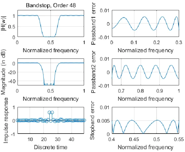
3.3.4.2 48th-order Bandstop Digital Filter ... 37

3.4 Conclusion ... 39

CHAPTER 4 General FIR Digital Filter Design Using Multiobjective Cuckoo

Search Algorithm ... 40

4.2 Multiobjective Cuckoo Search Algorithm ... 41

4.3 Design of General FIR Digital Filters ... 42

(9)

viii

4.4.1.1 Lowpass Digital Filter with Group Delay in Passband at 10 ... 44

4.4.2 24th-order Highpass Digital Filters ... 54

4.4.2.1 Hihjpass Digital Filter with Group Delay in Passband at 10 ... 54

4.4.2.2 Highpass Digital Filter with Group Delay in Passband at 12 ... 57

4.4.2.3 Highpass Digital Filter with Group Delay in Passband at 14 ... 61

4.4.3 24th-order Bandpass Digital Filters ... 64

4.4.3.1 Bandpass Digital Filter with Group Delay in Passband at 10 ... 64

4.4.4 24th-order Bandstop Digital Filters ... 74

4.4.4.1 Bandstop Digital Filter with Group Delay in Passband at 10 ... 74

CHAPTER 5 IIR Digital Filter Design Using Constrained Multiobjective Cuckoo

Search Algorithm ... 85

5.2 Constrained Multiobjective Cuckoo Seach Algorithm ... 85

5.3 Design of IIR Digital Filters ... 86

5.4.1 Example 1... 91

5.4.2 Example 2... 94

5.4.3 Example 3... 98

CHAPTER 6 Conclusion Remarks ... 102

REFERENCES ... 103

(10)

ix

LIST OF TABLES

Table 3.1 Pseudocode of Cuckoo Search Algorithm ... 20

Table 3.2 Filter specifications and CSA parameters ... 22

Table 3.3 LP-FIR1 digital filter cutoff frequencies ... 23

Table 3.4 Frequency grid for LP-FIR1 digital filter design ... 23

Table 3.5 Coefficients of 24th-order LP-FIR1 lowpass digital filter ... 23

Table 3.6 Design results of 24th-order LP-FIR1 lowpass digital filter ... 24

Table 3.7 Computational record of 24th-order LP-FIR1 lowpass digital filter ... 24

Table 3.8 Coefficients of 48th-order LP-FIR1 lowpass digital filter ... 25

Table 3.9 Design results of 48th-order LP-FIR1 lowpass digital filter ... 26

Table 3.10 Computational record of 48th-order LP-FIR1 lowpass digital filter ... 26

Table 3.11 Coefficients of 24th-order LP-FIR1 highpass digital filter ... 27

Table 3.12 Design results of 24th-order LP-FIR1 highpass digital filter ... 28

Table 3.13 Computational record of 24th-order LP-FIR1 highpass digital filter ... 28

Table 3.14 Coefficients of 48th-order LP-FIR1 highpass digital filter ... 29

Table 3.15 Design results of 48th-order LP-FIR1 highpass digital filter ... 30

Table 3.16 Computational record of 48th-order LP-FIR1 highpass digital filter ... 30

Table 3.17 Coefficients of 24th-order LP-FIR1 bandpass digital filter ... 31

Table 3.18 Design results of 24th-order LP-FIR1 bandpass digital filter ... 32

Table 3.19 Computational record of 24th-order LP-FIR1 bandpass digital filter ... 32

Table 3.20 Coefficients of 48th-order LP-FIR1 bandpass digital filter ... 33

Table 3.21 Design results of 48th-order LP-FIR1 bandpass digital filter ... 34

Table 3.22 Computational record of 48th-order LP-FIR1 bandpass digital filter ... 34

Table 3.23 Coefficients of 24th-order LP-FIR1 bandstop digital filter ... 35

Table 3.24 Design results of 24th-order LP-FIR1 bandstop digital filter ... 36

Table 3.25 Computational record of 24th-order LP-FIR1 bandstop digital filter ... 36

Table 3.26 Coefficients of 48th-order LP-FIR1 bandstop digital filter ... 37

Table 3.27 Design results of 48th-order LP-FIR1 bandstop digital filter ... 38

Table 3.28 Computational record of 48th-order LP-FIR1 bandstop digital filter ... 38

Table 4.1 Parameters of MOCSA and NSGA-III ... 43

Table 4.2 G-FIR digital filter cutoff frequencies ... 43

Table 4.3 Frequency grid for G-FIR digital filter design ... 43

(11)

x

Table 4.5 Magnitude error of lowpass digital filter with group delay in passband at 10 .. 45

Table 4.6 Group delay error of lowpass digital filter with group delay in passband at 10 ... 45

Table 4.7 Computational record of lowpass digital filter with group delay in passband at 10 ... 45

Table 4.8 Coefficients of lowpass digital filter with group delay in passband at 12 ... 47

Table 4.9 Magnitude error of lowpass digital filter with group delay in passband at 12 .. 48

Table 4.12 Coefficients of lowpass digital filter with group delay in passband at 14 ... 51

Table 4.13 Magnitude error of lowpass digital filter with group delay in passband at 14 ... 52

Table 4.16 Coefficients of highpass digital filter with group delay in passband at 10 ... 54

Table 4.17 Magnitude error of highpass digital filter with group delay in passband at 10 ... 55

Table 4.18 Group delay error of highpass digital filter with group delay in passband at 10 ... 55

Table 4.19 Computational record of highpass digital filter with group delay in passband at 10 ... 55

Table 4.22 Group delay error of highpass digital filter with group delay in passband at 12 ... 58

(12)

xi

Table 4.28 Coefficients of bandpass digital filter with group delay in passband at 10 .... 64

Table 4.29 Magnitude error of bandpass digital filter with group delay in passband at 10 ... 65

Table 4.30 Group delay error of bandpass digital filter with group delay in passband at 10 ... 65

Table 4.31 Computational record of bandpass digital filter with group delay in passband at 10 ... 65

Table 4.40 Coefficients of bandstop digital filter with group delay in passband at 10 ... 74

Table 4.41 Magnitude error of bandstop digital filter with group delay in passband at 10 ... 75

Table 4.42 Group delay error of bandstop digital filter with group delay in passband at 10 ... 75

Table 4.43 Computational record of bandstop digital filter with group delay in passband at 10 ... 75

(13)

xii

Table 4.51 Computational record of bandstop digital filter with group delay in passband at 14 ... 82

Table 5.1 Parameters of constrained MOCSA ... 90

Table 5.2 Frequency grid for IIR digital filter design ... 91

Table 5.3 Filter specification of designed IIR lowpass digital filter in Example 1 ... 91

Table 5.4 Performance requirements of designed IIR lowpass filter in Example 1 ... 91

Table 5.5 Design results of the IIR lowpass digital filter in Example 1 ... 92

Table 5.6 Computational record of designed IIR lowpass digital filter in Example 1 ... 92

Table 5.7 Coefficients of designed IIR lowpass digital filter in Example 1 ... 92

Table 5.8 Filter specification of designed IIR highpass digital filter in Example 2 ... 94

Table 5.9 Performance requirements of designed IIR highpass filter in Example 2 ... 95

Table 5.10 Design results of the IIR highpass digital filter in Example 2 ... 95

Table 5.11 Computational record of designed IIR highpass digital filter in Example 2 ... 95

Table 5.12 Coefficients of designed IIR highpass digital filter in Example 2 ... 95

Table 5.13 Filter specification of designed IIR bandpass digital filter in Example 3 ... 98

Table 5.14 Performance requirements of designed IIR bandpass filter in Example 3 ... 98

Table 5.15 Design results of the IIR bandpass digital filter in Example 3 ... 98

Table 5.16 Computational record of designed IIR bandpass digital filter in Example 3 .. 99

(14)

xiii

LIST OF FIGURES

Fig. 1.1 Input-filtering-output correspondence of a digital filter for its impluse response . 3

Fig. 1.2 Magnitude response of an ideal lowpass digital filter ... 4

Fig. 1.3 Magnitude response of an ideal highpass digital filter ... 5

Fig. 1.4 Magnitude response of an ideal bandpass digital filter ... 6

Fig. 1.5 Magnitude response of an ideal bandstop digital filter ... 7

Fig. 2.1 Configuration of a chromosome in GA ... 11

Fig. 2.2 Initialization of a chromosome in GA ... 12

Fig. 2.3 Roulette wheel for a population in GA ... 13

Fig. 2.4 An example of elite selection in GA ... 13

Fig. 2.5 Crossover operation in GA ... 14

Fig. 2.6 Mutation operation in GA ... 15

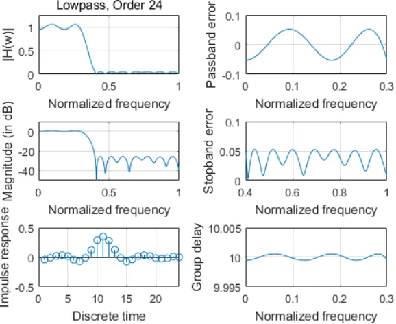
Fig. 3.1 Magnitude response, impulse response, the passband and stopband errors of designed 24th-order LP-FIR1 lowpass digital filter ... 24

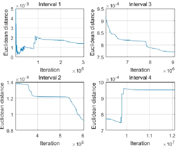
Fig. 3.2 Convergence curve of designed 24th-order LP-FIR1 lowpass digital filter ... 25

Fig. 3.3 Magnitude response, impulse response, the passband and stopband errors of designed 48th-order LP-FIR1 lowpass digital filter ... 26

Fig. 3.4 Convergence curve of designed 48th-order LP-FIR1 lowpass digital filter ... 27

Fig. 3.5 Magnitude response, impulse response, the passband and stopband errors of designed 24th-order LP-FIR1 highpass digital filter ... 28

Fig. 3.6 Convergence curve of designed 24th-order LP-FIR1 highpass digital filter ... 29

Fig. 3.7 Magnitude response, impulse response, the passband and stopband errors of designed 24th-order LP-FIR1 highpass digital filter ... 30

Fig. 3.8 Convergence curve of designed 48th-order LP-FIR1 highpass digital filter ... 31

Fig. 3.9 Magnitude response, impulse response, the passband and stopband errors of designed 24th-order LP-FIR1 bandpass digital filter ... 32

Fig. 3.10 Convergence curve of designed 24th-order LP-FIR1 bandpass digital filter .... 33

Fig. 3.11 Magnitude response, impulse response, the passband and stopband errors of designed 48th-order LP-FIR1 bandpass digital filter ... 34

Fig. 3.12 Convergence curve of designed 48th-order LP-FIR1 bandpass digital filter .... 35

Fig. 3.13 Magnitude response, impulse response, the passband and stopband errors of designed 24th-order LP-FIR1 bandstop digital filter ... 36

Fig. 3.14 Convergence curve of designed 24th-order LP-FIR1 bandstop digital filter .... 37

(15)

xiv

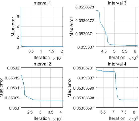
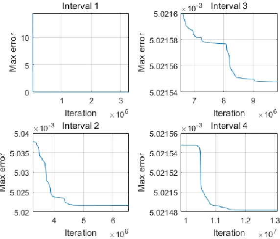
Fig. 3.16 Convergence curve of designed 48th-order LP-FIR1 bandstop digital filter .... 39

Fig. 4.1 Magnitude response, impulse response, the passband and stopband errors of designed G-FIR lowpass digital filter with group delay in passband at 10 obtained by MOCSA ... 46

Fig. 4.2 Magnitude response, impulse response, the passband and stopband errors of designed G-FIR lowpass digital filter with group delay in passband at 10 obtained by NSGA-III ... 46

Fig. 4.3 Convergence curve of designed G-FIR lowpass digital filter with group delay in passband at 10 obtained by MOCSA ... 47

Fig. 4.10 Magnitude response, impulse response, the passband and stopband errors of designed G-FIR highpass digital filter with group delay in passband at 10 obtained by MOCSA ... 56

Fig. 4.11 Magnitude response, impulse response, the passband and stopband errors of designed G-FIR highpass digital filter with group delay in passband at 10 obtained by NSGA-III ... 56

Fig. 4.12 Convergence curve of designed G-FIR highpass digital filter with group delay in passband at 10 obtained by MOCSA ... 57

(16)

xv

Fig. 4.17 Magnitude response, impulse response, the passband and stopband errors of designed G-FIR highpass digital filter with group delay in passband at 14 obtained by NSGA-III ... 63

Fig. 4.19 Magnitude response, impulse response, the passband and stopband errors of designed G-FIR bandpass digital filter with group delay in passband at 10 obtained by MOCSA ... 66

Fig. 4.20 Magnitude response, impulse response, the passband and stopband errors of designed G-FIR bandpass digital filter with group delay in passband at 10 obtained by NSGA-III ... 66

Fig. 4.21 Convergence curve of designed G-FIR bandpass digital filter with group delay in passband at 10 obtained by MOCSA ... 67

(17)

xvi

Fig. 4.29 Magnitude response, impulse response, the passband and stopband errors of designed G-FIR bandstop digital filter with group delay in passband at 10 obtained by NSGA-III ... 76

Fig. 4.30 Convergence curve of designed G-FIR bandstop digital filter with group delay in passband at 10 obtained by MOCSA ... 77

Fig. 4.31 Magnitude response, impulse response, the passband and stopband errors of designed G-FIR bandstop digital filter with group delay in passband at 12 obtained by MOCSA ... 79

Fig. 4.34 Magnitude response, impulse response, the passband and stopband errors of designed G-FIR bandstop digital filter with group delay in passband at 14 obtained by MOCSA ... 82

Fig. 5.1 Magnitude, group delay, magnitude errors and group delay errors of designed IIR lowpass digital filter in Example 1 obtained by constrained MOCSA ... 93

Fig. 5.2 Convergence curve of designed IIR lowpass digital filter in Example 1 obtained by constrained MOCSA ... 94

Fig. 5.3 Magnitude, group delay, magnitude errors and group delay errors of designed IIR highpass digital filter in Example 2 obtained by constrained MOCSA ... 97

Fig. 5.4 Convergence curve of designed IIR highpass digital filter in Example 1 obtained by constrained MOCSA ... 97

Fig. 5.5 Magnitude, group delay, magnitude errors and group delay errors of designed IIR bandpass digital filter in Example 3 obtained by constrained MOCSA ... 100

(18)

xvii

LIST OF ABBREVIATIONS/SYMBOLS

FIR Finite Impulse Response

IIR Infinite Impulse Response

CSA Cuckoo Search Algorithm

MOCSA Multiobjective Cuckoo Search Algorithm

NSGA-III Non-dominated Sorting Genetic Algorithm III

GA Genetic Algorithm

DE Differential Evolution

PSO Particle Swarm Optimization

LP-FIR Linear-phase FIR

(19)

1

CHAPTER 1 Introduction to Digital Filters

1.1 Introduction

A digital filter is a mathematical system which operates numerical calculation on a discreet-time sampled signal to extract or remove its specific components. A continuous-discreet-time analog signal is usually sampled by a certain frequency to be converted into a corresponding set of discreet numerical sequences. These sequences can be operated by filtering processing in a digital filter system to obtain the desired components of a signal.

Compared to analog filters, digital filters contain three representative advantages including:

Reliability: The characteristics of digital filters stay stable without disadvantages of aging or tolerance. The coefficients of a designed digital filters can be permanently fixed and used.

Accuracy: The word length of filter coefficients can be precisely controlled to assure its accuracy. A longer word length, especially with more decimal parts, leads to higher accuracy. Approximation of ideal sharp cutoff is available if sufficiently long word length is provided.

Flexibility: Filtering characteristics are easy to modify by changing the filter coefficients.

With these advantages, digital filters play a very important role in nowadays society. Digital filters are being used in plenty of practical applications, such as communication, electrical systems and astronautic industry, etc.

In view of the finiteness of impulse response, digital filters can be divided into finite impulse response (FIR) digital filters and infinite impulse response (IIR) digital filters. Meanwhile, in view of the filter shape, digital filters mainly include four types called lowpass, highpass, bandpass and bandstop filters.

1.2 Analog-to-digital Conversion

For a continuous-time analog signal 𝑥(𝑡), its sampled signal 𝑥𝑠(𝑡) with a period of 𝑇 seconds can be represented to be a set of numerical impulses that

𝑥𝑠(𝑡) = 𝑥(𝑡) ∑∞𝑛=−∞𝛿(𝑡 − 𝑛𝑇)= ∑∞𝑛=−∞𝑥(𝑛𝑇)𝛿(𝑡 − 𝑛𝑇) (1.1)

where 𝛿(𝑡) is a unit impulse function that

𝛿(𝑡) = {1 𝑡 = 0

0 𝑡 ≠ 0 (1.2)

The sampling frequency 𝑤𝑠 is calculated by

𝑤𝑠= 2𝜋

(20)

2

1.2.1 Limitation of Sampling Frequency

An original signal 𝑥(𝑡) can be decomposed into a series of components with different

frequencies. Let the highest frequency among those components as 𝑤𝑚, then the sampling

frequency 𝑤𝑠 must follow the below limitation that

𝑤𝑠≥ 2𝑤𝑚 (1.4)

1.2.2 Normalized Frequency

For the mathematical expression of a digital filter system, the analog frequency 𝑓 (in samples/second) is often normalized with respect to the sampling frequency 𝑓𝑠 (in

samples/second) such that a normalized digital frequency 𝑣 (in radians/sample) can be derived as [1]

𝑣 = 2𝑓/𝑓𝑠 (1.5)

When the previous analog frequency is equal to the sampling frequency that 𝑓 = 𝑓𝑠, then we

have normalized frequency 𝑣 = 2 corresponding to 2𝜋 in radians/sample to represent a cycle of

the base band in frequency spectrum.

For convenient visualization due to the periodicity of frequency band with a period of 2 (in

normalized frequency), the normalized frequency adopts

𝑤 =𝑣

2, 0 ≤ 𝑣 ≤ 2 (1.6)

where the half normalized frequency 𝑤 (in half-cycle/sample) is in the range of 0 to 1.

1.3 Z-transform to A Digital Filter

A digital filter can be closely expressed by a transfer function in frequency domain for further design, optimization and realization. The transfer function of a digital filter can be calculated by taking the 𝑧-transform [1] of its impulse response which is a discrete output signal with an

impulse input of magnitude “1” at the beginning input but “0” at all latter inputs to a digital filter.

The impulse response of a digital filter can be expressed as

𝒉 = ∑∞𝑛=0ℎ(𝑛𝑇)𝛿(𝑡 − 𝑛𝑇) (1.7)

where 𝑇 is the sampling period; ℎ(𝑛𝑇) represents the 𝑛th sampled discrete impulse response. For simplicity, (1.7) can be simplified as

𝒉 = ∑∞𝑛=0ℎ(𝑛)𝛿(𝑡 − 𝑛𝑇) (1.8)

(21)

3

Fig. 1.1 Input-filtering-output correspondence of a digital filter for its impulse response

The z-transform of a digital filter can be expressed as

𝐻(𝑤) = ∑∞𝑛=0ℎ(𝑛)𝑧−𝑛|𝑧=𝑒𝑗𝑤𝑇 = ∑∞𝑛=0ℎ(𝑛)𝑒−𝑗𝑛𝑤𝑇 (1.9)

Where 𝐻(𝑤) is named as the frequency response of a digital filter.

Normally, the coefficients of the transfer function of a digital filter are real numbers, which

result in an even function of frequency for its magnitude response while an odd function for its

phase response that [1]

|𝐻(−𝑤)| = |𝐻(𝑤)| (1.10)

𝜃(−𝑤) = −𝜃(−𝑤) (1.11)

(22)

4

1.4 Four Main Types of Ideal Filter Shapes [1]

1.4.1 Ideal Lowpass Digital Filter

An ideal lowpass digital filter has a magnitude response of one at lower frequencies but that of zero at higher frequencies. The magnitude response of an ideal lowpass digital filter with an ideal cutoff frequency 𝑤𝑐 is defined as

|𝐻_𝐿𝑃(𝑤)| = {1 for |𝑤| ≤ 𝑤𝑐

0 for |𝑤| ≥ 𝑤𝑐 (1.12)

Fig. 1.2 Magnitude response of an ideal lowpass digital filter

The magnitude response of an ideal lowpass digital filter is shown in Fig. 1.2. The magnitude

response in passband is limited within the range of 1 − 𝛿𝑝 to 1 + 𝛿𝑝 and the magnitude response

in stopband is limited within the range of 0 to 𝛿𝑠. 𝛿𝑝 represents the acceptable peak error in

passband while 𝛿𝑠 represents that in stopband. The ideal cutoff frequency shall normally be 𝑤𝑐 but

practically the magnitude response can not be strictly sharp at frequency 𝑤𝑐. Hence, a passband

cutoff frequency 𝑤𝑝 and a stopband cutoff frequency 𝑤𝑠 are used to retain a transition band, which

formulates a more achievable requirement for approximation.

1.4.2 Ideal Highpass Digital Filter

An ideal highpass digital filter has a magnitude response of zero at lower frequencies but that

of one at higher frequencies. The magnitude response of an ideal highpass digital filter with an

ideal cutoff frequency 𝑤𝑐 is defined as

|𝐻𝐻𝑃(𝑤)| = {0 for |𝑤| ≤ 𝑤_{1 for 𝑤} 𝑐

(23)

5

Fig. 1.3 Magnitude response of an ideal highpass digital filter

The magnitude response of an ideal highpass digital filter is shown in Fig. 1.3. The magnitude

in stopband is limited within the range of 0 to 𝛿𝑠. 𝛿𝑠 represents the acceptable peak error in

stopband while 𝛿𝑝 represents that in passband. The ideal cutoff frequency shall normally be 𝑤𝑐 but

practically the magnitude response can not be strictly sharp at frequency 𝑤𝑐. Hence, a stopband

cutoff frequency 𝑤𝑠 and a passband cutoff frequency 𝑤𝑝 are used to retain a transition band, which

1.4.3 Ideal Bandpass Digital Filter

An ideal bandpass digital filter has a magnitude response of zero at lower and higher

frequencies but that of one at middle frequencies. The magnitude response of an ideal bandpass

digital filter with an ideal cutoff frequency 𝑤𝑐 is defined as

|𝐻𝐵𝑃(𝑤)| = {

0 for |𝑤| ≤ 𝑤𝑐1

1 for 𝑤𝑐1≤ |𝑤| ≤ 𝑤𝑐2

0 for 𝑤𝑐2≤ |𝑤| ≤ 𝜋

(24)

6

Fig. 1.4 Magnitude response of an ideal bandpass digital filter

The magnitude response of an ideal bandpass digital filter is shown in Fig. 1.4. The magnitude

in stopband is limited within the range of 0 to 𝛿𝑠. 𝛿𝑠 represents the acceptable peak error in

stopband while 𝛿𝑝 represents that in passband. The ideal cutoff frequency shall normally be 𝑤𝑐1

and 𝑤𝑐2 but practically the magnitude response can not be strictly sharp at both frequencies 𝑤𝑐1

and 𝑤𝑐2. Hence, two stopband cutoff frequencies 𝑤𝑠1 and 𝑤𝑠2 as well as two passband cutoff

frequencies 𝑤𝑝1 and 𝑤𝑝2 are used to retain two transition bands on both sides of passband, which

1.4.4 Ideal Bandstop Digital Filter

An ideal bandstop digital filter has a magnitude response of one at lower and higher

frequencies but that of zero at middle frequencies. The magnitude response of an ideal bandstop

digital filter with an ideal cutoff frequency 𝑤𝑐 is defined as

|𝐻𝐵𝑆(𝑤)| = {

1 for |𝑤| ≤ 𝑤𝑐1

0 for 𝑤𝑐1≤ |𝑤| ≤ 𝑤𝑐2

1 for 𝑤𝑐2≤ |𝑤| ≤ 𝜋

(25)

7

Fig. 1.5 Magnitude response of an ideal bandstop digital filter

The magnitude response of an ideal bandstop digital filter is shown in Fig. 1.5. The magnitude

in stopband is limited within the range of 0 to 𝛿𝑠. 𝛿𝑝 represents the acceptable peak error in

passband while 𝛿𝑠 represents that in stopband. The ideal cutoff frequency shall normally be 𝑤𝑐1

and 𝑤𝑐2 but practically the magnitude response can not be strictly sharp at both frequencies 𝑤𝑐1

and 𝑤𝑐2. Hence, two passband cutoff frequencies 𝑤𝑝1 and 𝑤𝑝2 as well as two stopband cutoff

frequencies 𝑤𝑠1 and 𝑤𝑠2 are used to retain two transition bands on both sides of stopband, which

(26)

8

CHAPTER 2 Introduction to Evolutionary Algorithms

2.1 Introduction

In this chapter, a special type of practical problems called optimization problems is discussed.

For solving an optimization problem, an effective kind of methods, evolutionary algorithms, is

introduced. The basic introduction of evolutionary algorithms includes biological origin,

correspondence to computational optimization process and development of some typical

evolutionary algorithms. Finally, the basic methodologies of a general evolutionary algorithm are

described in detail where Genetic Algorithm (GA) is used as an example for clear illustration.

2.2 Optimization Problems

For a computational system, if a specific input is provided, this system would process such

input through some computational steps and results in a corresponding output [2]. Sometimes this

computational system may be so complicated that it is not easy to describe its computational steps

directly. However, once this system is fully configurated, it is very simple to obtain the output from

a given input. Input, computational steps and output are the three main components of such

computational system.

However, some computation systems are mainly forward-going and can not be simply inverted.

although it is easy to proceed the input-computation-output process, the reversed operation of

finding the input of an obtained output may be very difficult. It may require much more calculations

trying to backtrack the original input through a set of reversed computational steps. An optimization

problem can be expressed as searching for the potential input which leads to a given output. It aims

at identifying a potentially particular solution by a sufficient search in an enormous space of

possibilities. Such space of possibilities induces a searching space which contains all possible

solutions as well as the optimal one that is being looked for. To find the optimal one in a searching

space, exhausting the whole space can be an inevitably successfully method but it is not realistic

when the searching space is huge enough.

Hence, some special techniques are required in order to find the optimal solution in a

searching space efficiently and accurately. Evolutionary algorithms are currently the most powerful

(27)

9

2.3 Evolutionary Algorithms

Evolutionary algorithm is a popular research area in intelligent computing. It derived from

biological natural evolution due to the powerful strength that various species overcome natural

selection in a fierce competing world for millions of years.

The Darwinian Principles demonstrate the basic process of natural evolution. For a certain

species in a living area, a population of individuals are always striving for survival and propagation.

The fitness for survival of each individual depends on the combined effect of environmental

mildness and its individual abilities of foraging food and protecting itself. That is to say, fitness

relates to a possibility of survival and reproduction. An individual with higher fitness is more

capable of surviving and have more chance to breed its offspring. As thousands of generations pass,

those with higher fitness due to some adaptive characteristics will be predominated and others

without such benefits would gradually die out. Then it means evolution on this species happens.

Similarly, in a computational optimization problem, a population of possible solutions from the

searching space are always being selected depending on their quality on how successful they can

solve a problem. A better solution has a higher chance to be kept while a worse one is very possible

to be abandoned. The correspondence between a biological evolutionary process and computational

optimization process is obvious that an environment corresponds to a problem and each individual

in a species population is related to a potential solution. The fitness for a biological individual

correlates with the achievement of a solution in an optimization problem. Such correspondence

inspired researchers with optimization algorithm based on evolutionary theory.

In the middle of 1960s, Lawrence Jerome Fogel firstly proposed Evolutionary Programming

[3] on computer algorithms and established the foundation of the development of further

evolutionary algorithms. Afterwards, several advancing evolutionary algorithms based on different

mechanisms had been published. A typical one is called Genetic Algorithm (GA) [4], which

simulates procedure of inheritance and mutation of genes. There were some prototypes of Genetic

Algorithm at that time. Holland summarized all related theories and thus put forward the modern

Genetic Algorithm. Besides Genetic Algorithm, other evolutionary algorithms have also gained a

lot of achievements. Differential Evolution (DE) [5] and Particle Swarm Optimization (PSO) [6]

are the very attractive ones. DE adopted differential operation on the changing of the population

while PSO simulates the movement of microscopic particles. Although these algorithms take

(28)

10

2.4 Basic Methodologies of An Evolutionary Algorithm

In this section, basic procedures of a viable evolutionary algorithm are presented. A successful

evolutionary algorithm should contain these procedures in adapt to any arbitrary optimization

problem. For clear clarification, Genetic Algorithm is taken as an illustration in which each of its

steps is illuminated in detail.

2.4.1 Configuration of Solutions

An optimization problem is usually based on a practical application. It often contains abstract

concepts or literal descriptions in the original problem context, which requires some suitable

operations to transform these information into mathematical expressions so that this problem is

capable of being numerical optimized.

First of all, any individual object shall be able to be appropriately converted or mapped into a

precise numerical expression corresponding to a specific algorithm, which creates a mapping

relation between the original objects and the population of solutions to be optimized [7]. For all

types of objects in the context problem, a solution shall contain a number of variables, each of

which is prescribed to represent a prescribed type of objects.

Secondly, an efficient optimization should have enough number of competitive solutions to

increase the efficiency on searching the optimal one. Those solutions are jointly regarded as a

population.

In GA, a solution is called a chromosome and all variables in a solution are named as genes.

Rather than the common decimal system, GA adopts binary system to express genes. The number

of binary bits for each gene depends on its desired precision. For a given solution, every variable

is coded by binary operation and afterward the binary bits of all variables will be configured

together as a single-stranded chromosome.

For example, a number “10” in decimal system could be represented as “1010” in binary

system. A number with fractional parts can also be binarily coded so long as the numbers of bits

for integer part and fractional part has been prescribed respectively in advance. For instance,

“14.375” can be represented coded by “1110” for integer part and “011” for fractional part. Then a binary chain “1110011” can be configured to represent the number “14.375” in decimal system,

where the former four bits are prescribed for integer part and the rest three bits for fractional part.

(29)

11

bits “1010000” represent “10” with “1010” as integer and “000” as decimal. A detailed

representation is shown in Figure 2.1.

Fig. 2.1 Configuration of a chromosome in GA

2.4.2 Objective Function

An objective function is an indicator which estimates the quality of a solution in an

optimization problem. It establishes a target for the whole population to aim at. In other words, all

the solutions collectively pursue the objective function and try to satisfy its requirement as possible

as they can. Normally, an objective function represents a formulistic measurement by quantizing

the levels of quality, which replaces abstract comparison.

In most of the optimization problems, the goal of an optimization procedure is maximizing or

minimizing the objective function as much as possible. In a maximization problem, the objective

function is always set as fitness function, which aims at searching for the most competitive solution

with the largest fitness value. On the other hand, in a minimization problem, the objective function

is always set as error function, which tries to find the optimum solution resulting in the least

variance from desired quality.

Similarly in GA, an objective function is used to evaluate the qualities of a population of

chromosomes. For example, in a minimization problem, a chromosome that leads to a smaller

output of the objective function is considered to be better while another chromosome with a larger

(30)

12

2.4.3 Initialization

It is necessary to provide the first generation of solutions to start a heuristic loop of

optimization. Generally, they can be initialized by random values drawn from a random function.

However, some special problems might have constraints or principles that help to generate a more

applicable set of solutions for initialization at the beginning. This step requires researches to check

which initialization method is more suitable.

For initialization of GA, Fig. 2.2 shows how a sample chromosome is initialized by a random

function.

Fig. 2.2 Initialization of a chromosome in GA

2.4.4 Elite Selection

Elite Selection is an important process to select elite solutions with better quality as candidates

of offspring’s parents. A better solution has a larger opportunity to generate its filial solution in

order to push quality improvements while a worse one can merely have a rather small possibility

to do so [7].

GA introduces a rotatable roulette wheel whose slots are of different sizes based on the

proportion of fitness value of every chromosome. Then the cumulative proportional value of each

chromosome is calculated according to their indices. Each time when trying to find an elite

chromosome, a random number is derived with the range of 0 to 1 representing a random value of

proportion. One chromosome with the smallest cumulative proportional value among those larger

than the given random number will be pick up as elite. One with a higher fitness value leads to a

larger proportion of fitness and a wider range in the cumulative proportional domain. It would

have a larger possibility to be selected. It should be noted that each round of elite selection is

(31)

13

parent population could have several same chromosomes. This would not cause a problem

because subsequent operations are designed to re-diversify the population. Fig 2.3 shows a

sample roulette wheel of a population and Fig. 2.4 shows an example of an elite selection.

Fig. 2.3 Roulette wheel for a population in GA

Fig. 2.4 An example of elite selection in GA

2.4.5 Variation for New Solutions

To further optimize a population, it is necessary to create new solutions from the existing ones.

By taking variation operations on a parent population, new solutions that inherit parts of their

parents’ characteristics and mutate with some specialities can be generated. In this case, two main

steps are required for generating a new population. One represents inheritance of parent solutions

while the other represents mutation of new specialities.

2.4.5.1 Inheritance

Inheritance of parent solutions is an operation that merge characteristics from two parent

solutions into one or two offspring solutions [7]. It decides which two solutions from a population

(32)

14

process is based on stochastic probabilities that parent solutions are randomly chosen and the

fragments that are being merged on parent solutions are randomly determined. In some algorithms,

a parthenogenetic principle is adopted that an offspring only inherits from one parent.

In GA, inheritance of parent solutions is equivalent to crossover on chromosomes. In each

time crossover is operated, two random parent chromosomes are fetched and one or two random

crossover points is then determined based on some stochastic decisions. A crossover point locates

the edge between the reserved parts and merging fragments on a parent chromosome. Afterward,

the two fetched parent chromosomes switch their merging fragments to each other and reserve the

rest parts. By mean of this, two new offspring chromosomes are generated with characteristics of

both of their parents. These operations will cycle until all the parent chromosomes have gone

through crossover where each one can only take crossover for one time. A new offspring population

after crossover is then created. Fig. 2.5 shows a simple crossover operation with one crossover

point on two sample chromosomes.

Fig. 2.5 Crossover operation in GA

2.4.5.2 Mutation

Mutation of new specialities applies on a unary solution and produce a mutant offspring with

probably slight changes. The mutation operation is always stochastic [7]. The number of mutant

points and their locations are both relied on a sequence of independent stochastic decisions. Each

location in one solution has an equal probability to mutate, and their decisions are all independent

from each other based on their respective deciding variables generated stochastically. The

probability of mutation is always small which would merely introduce a little new specialities and

reserve most of the characteristics of the original solution. A large probability of mutation might

lead to a totally fresh mutant solution with a large number of changes where its original

characteristics are swept out.

In GA, each bit of an offspring chromosome after crossover shall go through a

(33)

15

each bit is assigned with a random number, called mutation-deciding value, within the range of 0

to 1. These deciding values are then compared to mutant probability. If the

mutation-deciding value of a bit is smaller than mutant probability, this bit will mutate to an opposite binary

value such as “0” to “1” or “1” to “0”. Fig. 2.6 shows a simple mutation operation on a sample

chromosome.

Fig. 2.6 Mutation operation in GA

2.4.6 Survivor Determination

After the offspring solutions are generated, survivor determination which is similar to elite

selection will be carried out to determine a population of survivors with the highest quality among

a set of candidate solutions. However, survivor determination is rather deterministic that it only

concerns about the output of objective function resulting from each candidate solution. In other

words, survivor determination is a final evaluation of the output of objective functions related to

candidate solutions. Meanwhile, the set of candidate solutions might contain both the original

population and its offspring with an objective-based perspective or only reserve the offspring

solutions with an age-discriminational view. After survivor determination, the obtained population

of survivors will be taken to next generation and a new loop of evolutionary optimization procedure

will restart.

GA technically does not have the step of survivor determination. This is not only because the

number of offspring chromosomes is exactly the same as that of the original population but also

GA employs an age-discriminational view such that only the offspring chromosomes are reserved.

During the described steps in sections 2.4.4 and 2.4.5, GA keeps the same population size of

original population, selected parent population, offspring population after crossover and offspring

population after mutation. In this case, in order to deliver a population with the same population

(34)

16

2.4.7 Termination Criterion

A termination criterion is used to judge whether to stop the optimization procedure in case of

endless operations. For a practical optimization problem, a stochastic-based searching evolutionary

algorithm can not guarantee to obtain the global optimum. It is possible that an optimization could

never reach its goal that the value of objective function never reaches an expected level. This may

lead to an endless optimization process where time and resource of calculation are being wasted.

In this case, it is necessary to prescribe a termination criterion in advance to prevent possible

redundant optimization procedure such as maximum number of iterations or depleted CPU time,

(35)

17

CHAPTER 3 Linear Phase FIR Digital Filter Design Using Cuckoo Search Algorithm

3.1 Introduction of CSA

Cuckoo search algorithm (CSA) [8] - [9] is a successful evolutionary optimization method

which has been used in a large amount of numerical optimization problems [10]. CSA was first

proposed by Xin-She Yang in [8], who described the basic framework and internal approaches of

CSA. Afterward, Milan Tuba developed CSA with an a more sophisticated method for searching

step [10]. CSA was based on the biological fact that some cuckoo species has a special natural habit

of parasitic breeding [10]. For example, the Guira and Ani, will lay their eggs in shared nests, and

they may even take others’ eggs away so that their own eggs would have more chance to be hatched

[11]. CSA was soon implemented on practical engineering problems that its excellent performance

on several types of test functions was then presented in [12]. Considering other evolutionary

algorithms such as Genetic Algorithm and Particle Swarm Optimization, comparison shows that

CSA is superior to these existing algorithms for multimodal objective functions. On one hand, there

are fewer parameters to be pre-determined in CSA than in GA and PSO [8]. On the other hand, by

implementing a combination of global search and local search, CSA is capable of efficiently

traversing the whole searching space and accurately locating the local minima around a local space.

Recently, CSA and some other evolutionary algorithms have been successfully applied to the

designs of some typical types of FIR digital filters [13] - [15], which has raised people’s research

interest in this field.

In this chapter, more expansible and updated work on linear phase FIR digital filter design

using Cuckoo Search Algorithm is presented. This chapter firstly introduces the detailed description

of CSA including algorithm background, methodologies and calculation steps. Then it proposes the

configuration process of objective function based on linear-phase type-1 FIR digital filters. Finally,

lowpass, highpass, bandpass and bandstop digital filters at different order are taken as design

examples and their design results are compared to Park-McClellan Algorithm [16] - [18].

3.1.1 Biological Background of CSA

Cuckoos are some kinds of arboreal birds which have over 100 species. They can be mainly

classified into three families such as Cuculidae, Opisthocomidae and Musophagidae. Cuckoos have

widely spread around the world from Africa to east Asia. Their main food resource are forest insects

but some kinds of molluscs are also accessible [19].

Some cuckoo species are very reproductive due to their special aggressive brooding parasitism.

(36)

18

Most of the cuckoo don’t hatch their own eggs but cheat other host birds for resort [11]. They often

target at other host birds, who have just laid eggs. Afterward, cuckoos deposit their own deceitful

eggs into the host nest such that the host bird would take their place to hatch the eggs. Moreover, a

new born cuckoo chick can be very aggressive to expel the host bird’s egg in order to monopolize

the host bird’s feeding.

3.1.2 Biological Rules of CSA for Algorithm Realization

To realize the parasitism behavior of cuckoos into a computer algorithm, the below three rules

are regulated as

(1) Each time a cuckoo only lays one egg, and randomly chooses a foreign nest to deposit;

(2) High-quality eggs are regarded as best ones and will be inherited to next generations;

(3) The host nests available is limited, and there is a probability 𝑝𝑎∈ [0, 1] that a cuckoo egg

may be discovered by the host bird. In this case, the host bird can either dispose the egg or abandon

the nest and build a new nest [19].

3.1.3 Levy Flight

For random walking approximation, Levy flights [8] is a very competitive algorithm due to its

heavy-tailed probability distribution. Levy flights can be used to generate random numbers with a

random direction subjected to a uniform distribution and a step size that is drawn from the Levy

distribution [13]. In this case, a symmetric Levy stable distribution is a reliable method to generate

step size. By the use of Mantegna algorithm [8], the Levy flight with a parameter 𝛽 can be

calculated by

Levy(𝛽) =_|𝑣|𝑢_1/𝛽 (3.1)

where 𝑢 and 𝑣 are drawn from normal distributions [8]. Thus,

𝑢 = 𝑁(0, 𝜎𝑢2), 𝑣 = 𝑁(0, 𝜎𝑣2) (3.2)

where

𝜎𝑢= {

Γ(1+𝛽) sin(𝜋𝛽/2)

Γ[(1+𝛽)/2]∙𝛽∙2(𝛽−1)/2}

1/𝛽

(37)

19 and

Γ(𝑥) = ∫ 𝑒₀∞ −𝑡𝑡𝑥−1𝑑𝑡 (3.4)

3.1.4 Random Walk

A nest corresponds to an existing solution where several nests provide a number of potential

solutions. Each egg in a nest corresponds to a variable in an existing solution while a cuckoo egg

corresponds to a new generated value of a specific variable. If a cuckoo egg replaces a host egg, it

means a better solution with new updated variables in performance substitutes the old one. Usually,

an optimization problem involves a number of variables to be optimized. Thus, Cuckoo search

Algorithm has a multiple number of eggs in a nest [13]. A global explorative random walk and

local random walk is then applied to simulate the parasitic breeding behavior of cuckoos such that

new potentially better solution can be generated and compared. For a 𝑑 - dimensional optimization

problem, suppose the 𝑖th solution in iteration 𝑡 as

𝐱𝑖(𝑡) = [x𝑖1(𝑡) x𝑖2(𝑡) ⋯ x𝑖𝑑(𝑡)] 𝑇

(3.5)

The global walk for exploring the available searching space can be carried out by using Levy

flight described in (3.1) to (3.4) as

𝐱_𝑖𝑔(𝑡) = 𝐱_𝑖(𝑡) + 𝛼 × 𝐰⨂𝐋𝐞𝐯𝐲(𝛽)⨂(𝐱_𝑖(𝑡) − 𝐱_{𝑏𝑒𝑠𝑡}) (3.6)

where 𝛼 is a constant scale factor and 𝐰 is a vector comprised of random numbers subjected

to the standard normal distribution. 𝐋𝐞𝐯𝐲(𝛽) is a vector comprised of a set of numerical values

generated by Levy flight. The operator ⨂ means element-wise multiplications. 𝐱𝑏𝑒𝑠𝑡 is the best

solution that has ever been obtained from the beginning to current iteration [13].

On the other hand, the local random walk for searching a local minima is generated by

𝐱_𝑖𝑙(𝑡) = 𝐱_𝑖(𝑡) + 𝑟 × 𝐇(𝜖 − 𝑝_𝑎)⨂ (𝐱_𝑗(𝑡) − 𝐱_𝑘(𝑡)) (3.7)

where 𝐱𝑗(𝑡) and 𝐱𝑘(𝑡) are two distinct solutions randomly selected from the current population. 𝑟

and 𝜖 are random numbers evenly distributed in [0, 1]. 𝐇(𝜖 − 𝑝𝑎) is a vector comprised of

constant values either at one or zero determined by a Heaviside function that [13]

H(𝜖 − 𝑝𝑎) = {

1 𝜖 > 𝑝𝑎

(38)

20

At the end of each iteration, the best solution among 𝐱_𝑖𝑔(𝑡), 𝐱_𝑖𝑙(𝑡), and 𝐱𝑖(𝑡) is selected as

𝐱𝑖(𝑡 + 1) for the next iteration.

The pseudocode of CSA is listed in Table 3.1.

Table 3.1 Pseudocode of Cuckoo Search Algorithm

Steps Description

1 Set 𝑡 = 1; Set 𝛼, 𝛽, 𝑝𝑎; Initialize 𝐱(1);

2 Calculate the fitness values of 𝐱(𝑡);

3 Generate global walks 𝐱𝑔(𝑡) and calculate their fitness values;

4 Generate local walks 𝐱𝑙(𝑡) and calculate their fitness values;

5 Compare 𝐱𝑔(𝑡), 𝐱𝑙(𝑡), and 𝐱(𝑡) and update 𝐱(𝑡 + 1);

6 Compare each solution in 𝐱(𝑡 + 1) and update 𝐱𝑏𝑒𝑠𝑡;

7 If convergence criterion is satisfied, optimization procedure is completed; otherwise, return step 2;

8 Output the obtained optimal solution 𝐱𝑏𝑒𝑠𝑡.

3.2 Design of Linear-phase Type-1 FIR Digital Filters

An 𝑁th-order linear-phase type-1 FIR (LP-FIR1) filter [1] is an even 𝑁 and even symmetrical

FIR digital filter consisting of (𝑁 + 1) impulse responses as

𝐡 = [ℎ(0), ℎ(1), ℎ(2), … , ℎ(𝑛), … , ℎ(𝑁 − 1), ℎ(𝑁)]𝑇 (3.9)

According to its characteristic of even symmetry in impulse responses, it can be found that

ℎ(𝑛) = ℎ(𝑁 + 1 − 𝑛) for 𝑛 = 0, 1, 2, 3, … , (𝑁−2

2 ) (3.10)

The impulse response vector (3.9) can be represented by a distinct coefficient vector 𝐜 which

can be expressed as

𝐜 = [𝑐0, 𝑐1, 𝑐2, 𝑐3, … , 𝑐₍𝑁 2)

]

𝑇

= [ℎ (𝑁₂) , 2ℎ (𝑁₂− 1) , ⋯ , 2ℎ(2), 2ℎ(1), 2ℎ(0)]𝑇 (3.11)

The frequency response 𝐻(𝑤) of the LP-FIR1 filter can be expressed as

𝐻(𝑤) = 𝑒−𝑗(𝑁2)𝑤{ℎ (𝑁

2+ 1) + ∑ 2ℎ(𝑛)

𝑁−2 2

𝑛=0 cos [( 𝑁

2− 𝑛) 𝑤]} = 𝑒

−𝑗(𝑁

(39)

21

In (3.12), the magnitude response |𝐻(𝑤)| can be transformed as

|𝐻(𝑤)| = 𝐜𝑇_{𝐜𝐨𝐬 (𝑤)}_(3.13)

𝐜𝐨𝐬(𝑤) = [1 cos(𝑤) cos(2𝑤) ⋯ cos (𝑁

2𝑤)]

𝑇

(3.14)

The design of LP-FIR1 digital filter is to search for an optimal coefficient vector 𝐜 that

minimizes the objective function 𝑒(𝐜) in terms of maximum error which is defined as

min

𝐜 𝑒(𝐜) (3.15)

where

𝑒(𝐜) = max||𝐻(𝑤𝑖)| − 𝐻𝑑(𝑤𝑖)|

for 𝑤𝑖∈ Ω𝐼

(3.16)

where 𝐻𝑑(𝑤𝑖) is the ideal magnitude response of the desired LP-FIR1 digital filter; Ω𝐼 is the union

of band of interest including both passband and stopband.

For example, for a lowpass digital filter, the objective function 𝑒(𝐜) can be further

decomposed into error functions of magnitude in passband and stopband respectively as

𝑒(𝐜) = max (𝑒𝑝(𝐜), 𝑒𝑠(𝐜)) (3.17)

When operating on a union set of discrete sampling frequency points, 𝑤 ϵ Ω𝐼= [0, 𝑤𝑝] ∪

[𝑤s, 𝜋], the two error functions of magnitude response can be approximated by

𝑒𝑝(𝒄) = max

𝐼𝑝1 to 𝐼𝑝2||𝐻(𝒄, 𝑤𝑖

)| − 𝐻𝑑(𝑤𝑖)|

for 0 ≤ 𝑤𝑖≤ 𝑤𝑝

(3.18)

𝑒𝑠(𝒄) = max

𝐼𝑠1 to 𝐼𝑠2||𝐻(𝒄, 𝑤𝑖

)| − 𝐻𝑑(𝑤𝑖)|

for 𝑤𝑠≤ 𝑤𝑖 ≤ 𝜋

(3.19)

where 𝐻𝑑(𝑤𝑖) = 1 in passband and 𝐻𝑑(𝑤𝑖) = 0 in stopband.

Similarly, the objective function 𝑒(𝒄) of a highpass digital filter can be expressed as

𝑒(𝒄) = max (𝑒𝑠(𝐜), 𝑒𝑝(𝐜)) (3.20)

(40)

22

𝑒(𝒄) = max (𝑒𝑝1(𝐜), 𝑒𝑠(𝐜), 𝑒𝑝2(𝐜)) (3.21)

The objective function 𝑒(𝒄) of a bandstop digital filter can be expressed as

𝑒(𝒄) = max (𝑒𝑠1(𝐜), 𝑒𝑝(𝐜), 𝑒𝑠2(𝐜)) (3.22)

3.3 Design Examples and Results

In this section, linear-phase type-1 FIR lowpass, highpass, bandpass and bandstop digital

filters of order 24 and 48 are designed. All the filter coefficients are initialized randomly within a

specific range of lower bound and upper bound. Design results are compared favourably to

Park-McClellan Algorithm.

The linear-phase type-1 FIR lowpass, highpass, bandpass and bandstop digital filter

specifications, and CSA parameters are listed in Table 3.2. Lowpass, highpass, bandpass and

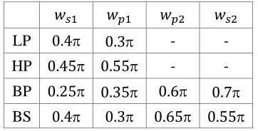
bandstop normalized cutoff frequencies are specified in Table 3.3. The adopt frequency grids for

optimization and for evaluating the peak errors of magnitude are shown in Table 3.4. The design

optimization is terminated when the value of the objective function from the best solution stays

unchanged during the last 10% continuous iterations. All the optimization designs are carried out

using an Intel(R) Core(TM) i7-5500U CPU, 2.40 GHz with 8GB RAM laptop computer.

Table 3.2 Filter specifications and CSA parameters

Symbol Description LP HP BP BS

𝑐_𝑘[𝑈] Upper bound of filter coefficients 0.45 0.675 0.45 1.275

𝑐_𝑘[𝐿] Lower bound of filter coefficients -0.95 -0.45 -0.33 -0.185 𝑁 Filter order 24 48 24 48 24 48 24 48 𝑁𝑐 Number of distinct coefficients 13 25 13 25 13 25 13 25

𝜏 Group delay 12 24 12 24 12 24 12 24 𝑃𝐶 CSA population size 25 25 25 25

𝛽 CSA parameter 1.5 1.5 1.5 1.5

𝛼 CSA parameter 0.01 0.01 0.01 0.01 𝑝𝑎 CSA parameter 0.25 0.25 0.25 0.25

Table 3.3 LP-FIR1 digital filter cutoff frequencies

Digital Filter Design Using Multiobjective Cuckoo Search Algorithm

Scholarship at UWindsor

Scholarship at UWindsor

Digital Filter Design Using Multiobjective Cuckoo Search

Digital Filter Design Using Multiobjective Cuckoo Search

Algorithm

Algorithm

Digital Filter Design Using Multiobjective Cuckoo Search Algorithm

By

Jiajun Liang

A Thesis

Submitted to the Faculty of Graduate Studies

through the Department of Electrical and Computer Engineering

in Partial Fulfillment of the Requirements for

the Degree of Master of Applied Science

at the University of Windsor

Windsor, Ontario, Canada

2018

Digital Filter Design Using Multiobjective Cuckoo Search Algorithm

by

Jiajun Liang

APPROVED BY:

____________________________ __________________

X. Guo

Odette School of Bussiness

______________________________________________

C

.

Chen

Department of Electrical and Computer Engineering

______________________________________________

H.K. Kwan, Advisor

Department of Electrical and Computer Engineering

DECLARATION OF ORIGINALITY

I hereby certify that I am the sole author of this thesis and that no part of this

thesis has been published or submitted for publication.

I certify that, to the best of my knowledge, my thesis does not infringe upon

anyone’s copyright nor violate any proprietary rights and that any ideas, techniques,

quotations, or any other material from the work of other people included in my thesis,

published or otherwise, are fully acknowledged in accordance with the standard

referencing practices. Furthermore, to the extent that I have included copyrighted

material that surpasses the bounds of fair dealing within the meaning of the Canada

Copyright Act, I certify that I have obtained a written permission from the copyright

owner(s) to include such material(s) in my thesis and have included copies of such

copyright clearances to my appendix.

I declare that this is a true copy of my thesis, including any final revisions,

as approved by my thesis committee and the Graduate Studies office, and that this

thesis has not been submitted for a higher degree to any other University or

ABSTRACT

Digital filters can be divided into finite impulse response (FIR) digital filters and

infinite impulse response (IIR) digital filters. Evolutionary algorithms are effective

techniques in digital filter designs. One such evolutionary algorithm is Cuckoo

Search Algorithm (CSA). The CSA is a heuristic algorithm which emulates a

special parasitic hatching habit of some species of cuckoos and have been proved

to be an effective method with various applications.

This thesis compares CSA with Park-McClellan algorithm on linear-phase FIR

Type-1 lowpass, highpass, bandpass and bandstop digital filter design.

Furthermore, a multiobjective Cuckoo Search Algorithm (MOCSA) is applied on

general FIR digital design with a comparison to Non-dominated Sorting Genetic

Algorithm III (NSGA-III). Finally, a constrained multiobjective Cuckoo Search

Algorithm is presented and used for IIR digital filter design. The design results of

the constrained MOCSA approach compares favorably with other state-of-the-art

optimization methods.

CSA utilizes Levy flight with wide-range step length for the global walk to assure

reaching the global optimum and the approach of local walk to orientate the

direction toward the local minima. Furthermore, MOCSA incorporates a method of

Euclidean distance combing objective-based equilibrating operations and the

searching for the optimal solution into one step and simplifies the procedure of

ACKNOWLEDGEMENTS

I am very grateful to Dr. H. K. Kwan for his patient instruction and invaluable

suggestions on this thesis. Dr. Kwan has enlightened me on the research of

evolutionary algorithms and in particularly the use of Cuckoo Search Algorithm

for designing linear phase FIR digital filters, asymmetric FIR digital filters and IIR

digital filters by multiobjective approach. He shares his precious experiences and

inspires me to make greater progress on my research area. Furthermore, I would

like to express my appreciation to Dr. Chunhong Chen and Dr. Xiaolei Guo for

their great insight and professional advice on my thesis. Besides, I expect to thank

TABLE OF CONTENTS

DECLARATION OF ORIGINALITY ... iii

ABSTRACT ... iv

__________