Type of the Paper (Article)
1
Evaluation of gridded multi-satellite precipitation
2
(TRMM-3B42-V7) estimation performance in the
3
Upper Indus Basin (UIB)
4
Asim Jahangir Khan1,2,*, Manfred Koch1 and Karen Milena Chinchilla1
5
1 Department of Geohydraulics and Engineering Hydrology, University of Kassel, Germany (Manfred Koch
6
[email protected], [email protected] ; Karen Milena Chinchilla - [email protected] -)
7
2 Department of Environmental Sciences, COMSATS Institute of Information Technology, Abbottabad
8
Campus.
9
* Correspondence: [email protected]; [email protected]; Tel.: +49-17631674283
10
11
Abstract: The present study aims to evaluate the capability of the TRMM-3B42-(V7) precipitation
12
product to estimate appropriate precipitation rates in the Upper Indus basin (UIB) and the analysis
13
of the dependency of the estimates’ accuracies on the time scale. To that avail statistical analyses
14
and comparison of the TMPA- products with gauge measurements in the UIB are carried out. The
15
dependency of the TMPA estimates’ quality on the time scale is analysed by comparisons of daily,
16
monthly, seasonal and annual sums for the UIB. The results show considerable biases in the TMPA-
17
(TRMM) precipitation estimates for the UIB, as well as high false alarms and miss ratios. The
18
correlation of the TMPA- estimates with ground-based gauge data increases considerably and
19
almost in a linear fashion with increasing temporal aggregation, i.e. time scale. The BIAS is mostly
20
positive for the summer season, while for the winter season it is predominantly negative, thereby
21
showing a slight over-estimation of the precipitation in summer and under-estimation in winter.
22
The results of the study suggest that, in spite of these discrepancies between TMPA- estimates and
23
gauge data, the use of the former in hydrological watershed modelling, endeavoured presently by
24
the authors, may be a valuable alternative in data- scarce regions, like the UIB, but still must be
25
taken with a grain of salt.
26
Keywords: Precipitation; Tropical Rainfall Measurement Mission (TRMM); Multi-satellite
27
Precipitation Analysis (TMPA); Upper Indus basin (UIB).
28
29
1.Introduction
30
The continued improvements in computation capabilities and the subsequent increase in the
31
development of spatially explicit and distributed models for expressing environmental phenomena
32
has necessitated the provision of more intensive and improved data for environmental variables both
33
in space and time. Two major issues, especially, in hydro-meteorological studies, are the possible
34
sparsity of data sampling points (gauge stations), and the discontinuities in the data and in the quality
35
of the temporal records. These issues are more frequent in mountainous regions with high altitudes
36
which are immensely challenging environments for measurements of precipitation, either through
37
remote-sensing or the traditional ground based methods, because of the difficult topography and the
38
highly variable weather and climatic conditions [1, 2]. Similarly, these and other reasons have
39
restricted many developing countries to have consistent spatial and temporal coverage for
ground-40
based precipitation measurements [2, 3] and make it difficult for them to achieve an effective spatial
41
coverage of rainfall [4, 5]. The consequent lack of good quality precipitation data, then turns out to
42
be a big hurdle for properly assessing impacts of climate change on water resources in these regions
43
[1].
44
As data with an acceptable gridded resolution of daily climatic variables are critical for
45
hydrological and water resources modeling [6, 7], managing the gaps in the data appropriately is
46
then the first stage of most climatological, environmental and hydrological studies [2]. This step is
47
also necessary to improve the spatial resolution for sparse gauge station data set, before using it as
48
an input for spatially-distributed rainfall-runoff models, because the gauge-based interpolation
49
methods, commonly used in hydrologic models, usually do not cover the spatial heterogeneity of the
50
variability of climatic variables in the catchment. These errors in the interpolated data field have then
51
the potential to significantly bias model calibrations and water balance calculations [6].
52
Fortunately, the continued scientific development is also showing new prospects in addressing
53
these issues. . For example, the advancements in the gathering and deriving climate data through
54
satellite remote sensing could provide a possible opportunity to mend some of the issues with regard
55
to the spatial coverage of climate data. That is why the use of satellite-based precipitation products,
56
individually, or in combination with land-based gauge data, has been increasingly recognized as a
57
very promising alternative to address the aforementioned problems [5]. Such precipitation products
58
prove to be of great value, especially, in developing countries with remote and high-altitude
59
locations, where conventional rain gauge- or weather data are of bad quality or have low coverage
60
[8][8].
61
There are numerous satellite-based precipitation products currently available with varying
62
degrees of accuracy. These include the Climate Prediction Center (CPC) morphing algorithm
63
(CMORPH) [9], the Global Satellite Mapping of Precipitation [10–12], the Naval Research Laboratory
64
Global Blended Statistical Precipitation Analysis [13] and the Tropical Rainfall Measuring Mission
65
(TRMM) Multisatellite Precipitation Analysis (TMPA) [14, 15] and a few others. Since their inception,
66
most of these gridded datasets have been evaluated for their suitability and usability for a specific
67
regions or intended uses. In general such investigations are specifically for mountainous regions, and
68
even less for the Hindukush, Karakurm and Himalays (HKH) region. In the HKH and the Upper
69
Indus Basin (UIB) region, most of the reported work related to evaluation of gridded precipitation
70
products, are suggestive of considerable biases in the gridded products in comparison to the gauge
71
records [16–19].
72
Additionally the quality, coverage or reprentetiveness of the available observed gauge records
73
have also been questioned and sometimes regarded below par [20–22] with considerable under
74
estimation of regional precipitation amounts especially at higher altitudes (Khan and Koch unpublished).(the
75
spatial distribution of estimated real precipitation by khan and Koch (unpublished) over study are is given in
76
the supplementary materials – Appendix-I while theVertical meteorological and cryspheric regimes in UIB
77
(modified from Hewitt 2007) is given in Appendix-II)
78
While, in most cases, these gridded global precipitation data sets are some interpolated version
79
of point measurements, (most often through geo-statistical procedures), they may only be useful for
80
regions where dense network of rain gauges are available, because otherwise, in absence of a dense
81
enough networks or over regions of complex topographies, the interpolated precipitation present a
82
very generalized destitution, not able to reflect on the prevalent orographic, surface or atmospheric
83
processes [19].
84
85
In comparison with the sparse gauge observations or the gridded data products, based on them,
86
satellite-based precipitation products, such as “Tropical Rainfall Measurement Mission” (TRMM)
87
“Multi-satellite Precipitation Analysis” (TMPA) (TRMM-3B42-(V7) have an inherent advantage, due
88
to their higher spatial coverage. However, they also have certain limitations, because they are indirect
89
estimates of rainfall, which depend on the cloud height and the properties of the cloud’s surfaces
(IR-90
algorithms) and on the integrated sparse and multi-source hydro-meteorological content (passive
91
microwave algorithms) [23, 15, 24]. Before such satellite-based data can be used with confidence, it is
92
therefore important to evaluate its accuracy or error characteristics by comparing it with data from
93
ground-based observations.
94
95
The current study was therefore aimed at assessing the skill of the TRMM precipitation dataset
96
observational network available, to evaluate its further processing and correction requirements or
98
suitability for subsequent use in hydrological modelling.
99
2.Materials and Methods
100
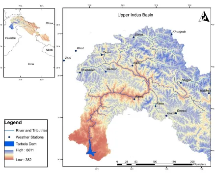
2.1. Study Area: “The Upper Indus River Basin (UIB)
101
The Indus River, one of the largest rivers in Asia with a total length of about 2880 km, has a
102
drainage area of about 912,000 km2 which extends across portions of India, China, Pakistan and
103
Afghanistan. The portion of the Indus that comprises the upper Indus river basin (UIB), with a logical
104
lower boundary at Tarbela Dam, is about 1125 km long and drains an area of about 170,000 km2 [25]
105
.106
Being a high-mountain region, the UIB contains the largest area of perennial glacial ice cover (22
107
000 km2) outside the polar regions of the earth, and which extends even further during the winter
108
season [26]. The altitude within the UIB ranges from as low as 455 m to a height of 8611 m and, as a
109
result, the climate varies greatly within the basin [27].
110
The summer monsoon has no significant effect on the basin, as almost 90% of its area lies in the
111
rain shadow of the Himalayan belt [28][20]. Except for the south-facing foothills, the intrusion of the
112
Indian-ocean monsoon is limited by the mountains, so that its influence weakens northwestward.
113
Subsequently, the climatic controls in the UIB are quite different from that in the Himalayas on the
114
eastern side. In fact, over the extent of the UIB, most of the annual precipitation originates in the west
115
and falls in winter and spring, whereas occasional rains are brought by the monsoonal incursions to
116
the trans-Himalayan areas, but so that even during the summer months the trans-Himalayan areas
117
do not obtain all their precipitation from the monsoons [29–32].
118
Climatic variables are usually strongly influenced by topographic altitude. Several studies have
119
pointed out that precipitation in the HKH region exhibits large changes over short distances and has
120
a considerable vertical gradient [33–36, 30, 29]. Thus the northern valley floors of the UIB are arid,
121
with annual precipitation of only 100-200 mm, but these totals increase with elevation and reach upto
122
600 mm at 4400 m, and even reach to an annual glacier accumulation rates of 1500 to 2000 mm at
123
5500 m altitude, according to some glaciological studies [29]. The average snow cover area in the
124
Upper Indus River Basin fluctuate between ~10% to 70%. Snow cover in the area is at a maximum of
125
70‒80% in the winter- (December to February) snow accumulation period and at a minimum 10‒15%
126
in the summer- (June to September) snow melt period [27]. Stream flow is generated by the
127
combination of the storm runoff in the lower parts of the upper Indus basin and the snow- and glacier
128
runoff from the higher parts of the UIB [37, 25].
129
2.1.1. TMPA Data (TRMM 3B42 V7)
132
In this study the TRMM 3B42 (V7) precipitation product is used. This product is basically a
133
calibration-based combination scheme for precipitation estimates from multiple satellites and
space-134
borne sensors, including infrared, microwave, radar data and gauge measurements. Though the
135
dataset has very good spatio-temporal resolution (0.25° × 0.25° grid, 3-hourly) and good global
136
coverage (latitude band 50°N to 50°S) and is available since 1998 to the recent past [15, 1] it also has
137
certain uncertainties, because the inputs on which they are based are indirect estimates of rainfall,
138
depending on the cloud height and the properties of the cloud surface (IR algorithms) and on the
139
integrated sparse and multi-source hydro-meteorological content (passive microwave algorithms)
140
[15, 24, 14].
141
During the current study, 3-hourly data from January 1, 1998 to December 31, 2008, were
142
summed to daily accumulated precipitation for each of the 0.25° X 0.25° grid box, which have a gauge
143
station, and evaluated for match with the corresponding gauge station’s observed daily accumulated
144
precipitation. As the observational network is scant, no TRMM grid box had more than one in situ
145
gauge station located in it.
146
2.1.2. Observed gauge data
147
In HKH region of Pakistan, observed in situ data are limited, and operated by different
148
organizations, mainly the Pakistan Meteorological Department (PMD) and Water and Power
149
Development Authority (WAPDA). The stations operated by PMD have daily time step climate data
150
available for longer periods (1947 to date) but with huge gaps and missing data in the record and
151
with only monthly data available freely for research purposes. Furthermore, all the PMD stations are
152
valley-based, at elevations below than 3000 m a.s.l. altitude, and therefore hardly represent the
153
frequency and amount of precipitation in the high-altitude areas. The climate stations, operated by
154
WAPDA, are fairly new and have considerably consistent, data over the time period, coinciding with
155
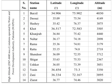
the TRMM product. These gauge stations are distributed almost evenly across the UIB inside Pakistan
156
and cover a wide range of elevations. During the current study, daily precipitation records of 14
157
meteorological stations operated by WAPDA were utilized for evaluation of TRMM estimates. Their
158
geographical attributes are given in Table 1. The evaluation limited to the duration of 1998 to 2008,
159
as the observed precipitation data could not be acquired for the period beyond 2008.
160
Table 1; Geographical attributes of the Precipitation gauge Network
161
S. No. Station name Latitude (◦) Longitude (◦) Altitude (m) H ig h A lt it u d e (2 3 6 7 – 44 4 0 m a .s. l. ) st a ti on s op era te d b y Wa te r a n d P ow er D ev el op m en t A u th ori ty , P a k ist a n (WA P D A )1 Burzil 34.906 75.902 4030
2 Deosai 35.09 75.54 4149
3 Hushey 35.42 76.37 3075
4 Khot 36.517 72.583 3505
5 Khunjrab 36.84 75.42 4440
6 Naltar 36.17 74.18 2898
7 Rama 35.36 74.81 3179
8 Rattu 35.15 74.8 2718
9 Shendoor 36.09 72.55 3712
10 Shigar 35.63 75.53 2367
11 Ushkor 36.05 73.39 3051
12 Yasin 36.454 73.3 3350
13 Zani 36.334 72.167 3895
14 Ziarat 36.77 74.46 3020
2.2. Methods
162
The quantitative comparison of the TRMM-estimates with ground rain-gauge station
163
observations is done by employing various widely used statistical indicators. These include the
164
correlation coefficient (R), the mean relative bias error (rBIAS), the mean bias error (MBE); mean
165
absolute error (MAE), and the root mean square error (RMSE). The R, rBAIS, MBE, MAE and RMSE
166
are defined in the following equations:
167
1 2 2 1 1(
)(
)
(
) ?
牋
(
)
n i i i n n i i i iT
T G
G
R
T
T
G
G
1
1
?
|
|)
n
i i
i
MAE
T
G
n
(3)
170
1
1
?
)
n
i i
i
MBE
T
G
n
(4)
171
2 1
1
(
)
n
i i
i
RMSE
T
G
n
(5)
172
where n is the number of samples, Ti are satellite-based precipitation, Gi are gauge-based
173
precipitation, and and ̅ are the corresponding means. Among these statistical indices, R shows
174
the degree of linear correlation between TRMM precipitation estimates and gauge observations;
175
MBE, MAE and rBIAS are used to assess the systematic bias, i.e. the deviation of the satellite
176
precipitation from the gauge observations, and the RMSE gives the magnitude of the average error
177
in relative terms.
178
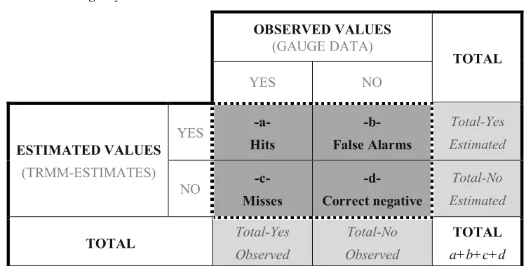
Table 2. Contingency table 2X2
179
OBSERVED VALUES (GAUGE DATA)
TOTAL
YES NO
ESTIMATED VALUES
(TRMM-ESTIMATES)
YES -a-
Hits
-b-
False Alarms
Total-Yes
Estimated
NO -c-
Misses
-d-
Correct negative
Total-No
Estimated
TOTAL Total-Yes Observed
Total-No
Observed
TOTAL
a+b+c+d
In addition, evaluations were also made for the daily TRMM estimates and gauge data, based
180
on a 2×2 contingency table (Table 2), by detecting rain events, no events, misses by TRMM and
false-181
alarms by the TRMM, over the Indus river basin.
182
We used a threshold of 0.3 mm/d, to differentiate precipitation and no precipitation events since
183
lower precipitation values may be the result of noise, as indicated by [30, 38] etc.
184
Based on these four indicators, orders as shown the table, several categorical statistical indices
185
are derived, including, accuracy (Ac), bias score or frequency bias index (FBI), probability of detection
186
(POD), false alarm ratio (FAR, critical success index (CSI) and true skill statistics (TSS) [39, 40] .
187
These are defined in the following equations:
188
a
d
Ac
Total
(6)
a
b
FBI
a
c
(7)190
a POD
a c
(8)
191
b
FAR
a
b
(9)192
a
CSI
a
b
c
(10)193
a
b
ad
bc
TSS
a b
c d
a b c d
(11)
194
where a represents the number of rainfall events that have been successfully estimated by
195
TRMM data (hits), b is the number of events incorrectly predicted as rain events by TRMM (false
196
alarms). c is the number actual events, that are missed by TRMM (Misses), while d is the number of
197
dry days or no-rainfall events identified successfully by the TRMM dataset. For each day, depending
198
on how the estimated and observed precipitation behave, any events above the given threshold (0.1
199
mm), is scored either as hit, miss, false-alarm or correct-negative.so that the rainfall is a hit if both,
200
|TRMM and observed, reach the threshold, False-alarm if if only the TRMM estimate reach the
201
threshold, miss if only the observed precipitation reaches it, and correct-negative if both are below
202
the threshold. The number of hits, fals-alarms, misses and correct-negatives ar used in eq-5 to 10, to
203
calculate the above mentioned statistical indices
204
Each of these indices provides a specific information of the two data sets compared. Thus Ac
205
indicates the fraction of estimates which is correct (range: 0 to 1. perfect score: 1); FBI indicates
206
whether the estimated dataset have a tendency to underestimate (FBI < 1) or to overestimate (FBI > 1)
207
rain events, POD quantifies the fraction of rain occurrences that is estimated correctly (range: 0 to 1.
208
perfect score: 1); FAR measures the fraction of false alarms in the satellite rain estimates (perfect score
209
of 0 and a range from 0 to 1. CSI measures the fraction of estimated events that are correctly predicted
210
(perfect score: 1) and a range from 0 to 1. Unlike all the aforementioned indices, TSS does not depend
211
on the frequency of climatological event and uses all elements in the contingency table (Table 2). Thus
212
TSS provides a measure of the accuracy of the estimates in terms of the probability of correct detection
213
of events or no events. In this case the range is form -1 to 1. Perfect score is 1, with 0 showing no skills
214
and a negative score means that the estimates are worse than a random forecast.
215
3.Results and discussion
216
The assessment of the reliability of the TRMM estimates and their comparisons with the rain
217
data from gauge station presented in this section has been done by three different methodologies, i.e.
218
(1) a statistical analysis, based on R, BIAS, MAE and RMSE for monthly, annual and seasonal data
219
aggregates, (2) categorical statistics daily data by computing Ac, FBI, POD, FAR, CSI and TSS, and (3)
220
visual comparison for monthly, annual and seasonal data.
221
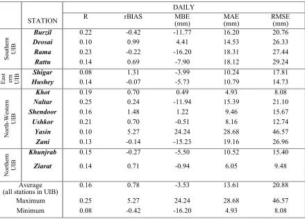
3.1. Statistical analysis
222
The results of the TRMM-assessment based on the statistical measures R, rBIAS, MBE, MAE and
223
RMSE, are given for daily data aggregation in Table 3, for monthly and annual data aggregation in
224
Table 4, and for seasonal aggregation in Table 5. The summer season include months of April, May,
225
June, July, August and September, while the remaining 6 months: October, November, December,
226
January, February and March are aggregated to represent Winter season.
227
It is evident from a first glance at the two tables that the TRMM performs overall rather poorly
228
values are only 0.16, 0.22, 0.22 and 0.20 for monthly, annual, and seasonal (summer and winter)
230
aggregation, respectively. Further specific results are discussed in the subsequent sub-sections
231
3.1.1. Skill Statistics for TRMM precipitation estimates (Daily aggregates)
232
The daily aggregates of TRMM precipitation estimates showed poor skill in matching observed
233
precipitation, with an average R of 0.16. Our comparison of the observed and TRMM daily rainfall
234
data shows highly variable MAE across the UIB, with a range ≥ 23 mm/day (Table-3). Values of MAE
235
were high throughout most of compared locations in UIB, with MAE ≤ 13 mm for the all stations
236
averaged rainfall, across the UIB. The North-Western parts of the UIB showed the highest and the
237
most variable MAE. The results showed that the TRMM data have huge under-estimation across most
238
of the UIB (average MBE of -3.53 mm), while the MBE values also showed a distinct spatial pattern
239
across the study area, with distinct under-estimation by TRMM estimates for all the studied locations
240
in the Eastern and Northern UIB; for the Southern UIB, TRMM estimates showed a high
under-241
estimation at all locations except one; while the stations located in the North-western UIB had a mixed
242
trend, where TRMM data showed moderate to high, under or over estimation at half (three) of the
243
locations each. The mean relative bias (rBIAS) at the different gauge location also followed an similar
244
pattern with huge veriations and ranging from a (-)tive 0.42 to as high as 5.27 (Table 3), while at
245
certain locations the relative bias was very high and at one location i.e. “Yasin” the rBais was even
246
more than 5 times the observed values. The RMSE for the daily time series were also very high and
247
showed large variations, ranging from and 8.08 to as high as 46.57 mm/day, with averages RSME of
248
20.88 for all locations averaged rainfall.
249
These results are in agreement with previous studies () as most of them have reported TRMM
250
product to underestimate rainfall amounts over the HKH region in general and even higher over the
251
western parts of HKH.
252
Table 3. Statistical analysis based on monthly and annual data aggregation.
253
DAILY
STATION R rBIAS (mm) MBE MAE (mm) RMSE (mm)
S
out
h
er
n
U
IB
Burzil 0.22 -0.42 -11.77 16.20 20.76
Deosai 0.10 0.99 4.41 14.53 26.33
Rama 0.23 -0.22 -16.20 18.31 27.44
Rattu 0.14 0.69 -7.90 18.12 29.24
E
as
t
er
n
U
IB Shigar 0.08 1.31 -3.99 10.24 17.81
Hushey 0.14 -0.07 -5.73 10.79 14.73
N
or
th
-W
es
te
rn
U
IB
Khot 0.19 0.70 0.49 4.93 8.08
Naltar 0.25 0.24 -11.94 15.39 21.10
Shendoor 0.16 1.48 1.22 9.46 15.67
Ushkor 0.21 0.70 -0.51 8.16 12.74
Yasin 0.10 5.27 24.24 28.68 46.57
Zani 0.13 -0.14 -15.23 19.16 26.96
N
or
the
rn
U
IB
Khunjrab 0.15 -0.27 -5.50 10.52 15.40
Ziarat 0.14 0.71 -0.94 6.05 9.48
Average (all stations in UIB)
0.16 0.78 -3.53 13.61 20.88
Maximum 0.25 5.27 24.24 28.68 46.57
Minimum 0.08 -0.42 -16.20 4.93 8.08
3.1.2. Skill Statistics for TRMM precipitation estimates (Monthly and annual aggregates)
255
The monthly and annual aggregated TRMM precipitation estimates also showed poor skill in
256
matching observed precipitation, but with considerably improved values for the Pearson correlation
257
coefficient R for all the studied locations and with an R of 0. 61 and 0.57 for average of rainfall at all
258
locations for monthly and annual aggregates, respectively.
259
Table 3. Statistical analysis based on monthly and annual data aggregation.
260
MONTHLY ANNUAL
STATION R rBIAS MBE
(mm) MAE (mm)
RMSE (mm)
R rBIAS MBE (mm)
MAE (mm)
RMSE (mm)
S
out
he
rn
U
IB
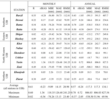
Burzil 0.55 -0.28 -56.80 58.73 112.81 0.43 -1.05 -391.5 391.5 407.7
Deosai 0.22 0.17 21.65 43.62 78.95 -0.37 0.24 146.6 201.4 234.6
Rama 0.54 -0.36 -78.26 79.54 165.86 0.78 -2.05 -538.5 538.5 574.8
Rattu 0.20 -0.20 -39.31 61.32 119.10 0.30 -0.58 -264.9 274.1 353.8
E
as
te
rn
U
IB Shigar 0.02 -0.21 -19.42 36.56 78.26 -0.11 -0.62 -133.2 179.7 249.8
Hushey 0.09 -0.24 -29.19 39.72 101.95 -0.15 -0.79 -193.2 230.3 339.6
N
ort
h
-W
es
te
rn
U
IB
Khot 0.51 -0.21 -26.52 39.47 74.14 0.29 -0.65 -182.0 242.7 250.9
Naltar 0.60 -0.31 -58.62 60.17 120.63 0.12 -1.32 -395.1 395.1 416.3
Shendoor 0.42 0.08 6.53 22.08 37.34 0.54 0.13 40.4 66.4 99.1
Ushkor 0.52 -0.03 -1.82 19.19 39.41 0.62 -0.05 -14.7 79.1 110.5
Yasin 0.21 1.36 118.35 126.68 241.25 0.10 0.72 806.0 806.0 827.5
Zani 0.49 -0.34 -75.05 77.98 154.91 0.52 -1.69 -508.3 508.3 532.6
N
ort
he
rn
U
IB
Khunjrab 0.39 0.05 2.26 13.13 23.40 -0.28 0.09 18.3 52.0 70.0
Ziarat 0.38 -0.07 -5.39 15.23 32.62 0.55 -0.15 -30.6 73.4 104.7 Average
(all stations in UIB) 0.61 -0.23 -9.09 14.15 20.98 0.57 -0.24 -117.3 117.3 134.1
Maximum 0.60 1.36 118.35 126.68 241.25 0.78 0.72 806.03 806.03 827.54
Minimum 0.02 -0.36 -78.26 13.13 23.40 -0.37 -2.05 -538.50 51.96 69.96
Our comparison of the observed and TRMM monthly and annual aggregated rainfall also
261
showed a highly variable MAE across the UIB, ranging from 13.13 mm/month to 126.68 mm/month,
262
in case of monthly aggregates and from -538.5 mm/year to 806.0 mm/year for annual aggregates
263
(Table-4). The values for MAE were high throughout most of compared locations in UIB, with an
264
average MAE of 14.15 mm/month and 117.3 mm/year, for the all locations average monthly and
265
annual rainfall across UIB, respectively. The spatial pattern of the errors observed in case of monthly
266
and annual aggregates as well as the predominant under-estimation at most location was similar to
267
that observed for the daily aggregates The North-Western parts of the UIB showed the highest and
268
the most variable MAE, while the TRMM data showed huge under-estimation across most of the UIB
269
(average MBE of a (-)tive 9.09 mm/month and -117.3 mm/year). The Eastern part UIB, showed a
270
distinct under-estimation by TRMM rainfall, across all the studied locations. In case of the Southern
271
UIB, the under-estimation was even higher but observed at three out of the four location, while at
272
one location (Deosai), an over estimation of 21.65 mm/month was observed. The stations located in
273
the North-western UIB had a mixed trend, where TRMM data showed a moderate to high,
under-274
estimation at four of the studied locations while the opposite in the remaining two, for both monthly
275
a mixed results with one station (Khunjrab) showing slight over-estimation (0.05 mm/month and 18.3
277
mm/year), while the other (Ziarat) showing a negative MBE (-0.07 mm/month and -30.6 mm/year).
278
3.1.3. Skill Statistics for TRMM precipitation estimates (Seasonal aggregates)
279
The seasonal statistical indices (Table 4) have comparable trends in terms of magnitude,
280
however, show a different pattern than the monthly- or annually computed ones. For example the in
281
summer season the TRMM showed positive BIAS for a few location where the monthly and annual
282
aggregates show a negative one (i.e. Rattu, Ushkor). Results for the winter season predominantly
283
show negative BIAS- values, similar to monthly and annual aggregation. The overall range of MBE
284
for the stations evaluated varies from—268.8 mm to 593.6 mm for the summer season and from -339.9
285
mm to 212.5 mm for winter season. The MBE for average rainfall across all location in UIB, was -5.18
286
and -96.51 mm for summer and winter respectively. These MBE value are comparatively lower in
287
case of summer season, are suggestive of a situation where the under or over-estimation occurring in
288
the different months of the seasons, cancel each other out to give an overall low MBE.
289
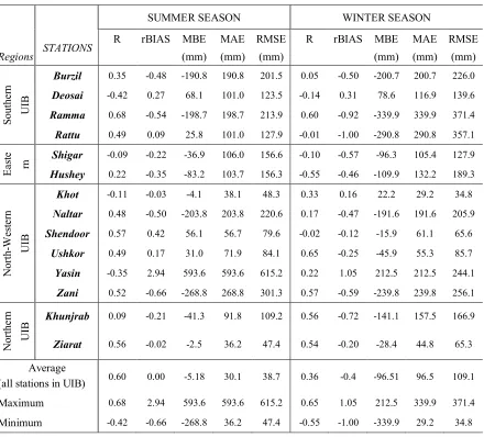
Table 4. Statistical analysis based on summer and winter season data aggregation
290
SUMMER SEASON WINTER SEASON
Regions STATIONS
R rBIAS MBE
(mm)
MAE
(mm)
RMSE
(mm)
R rBIAS MBE
(mm)
MAE
(mm)
RMSE
(mm)
S
out
he
rn
U
IB
Burzil 0.35 -0.48 -190.8 190.8 201.5 0.05 -0.50 -200.7 200.7 226.0
Deosai -0.42 0.27 68.1 101.0 123.5 -0.14 0.31 78.6 116.9 139.6
Ramma 0.68 -0.54 -198.7 198.7 213.9 0.60 -0.92 -339.9 339.9 371.4
Rattu 0.49 0.09 25.8 101.0 127.9 -0.01 -1.00 -290.8 290.8 357.1
E
as
te
rn Shigar
-0.09 -0.22 -36.9 106.0 156.6 -0.10 -0.57 -96.3 105.4 127.9
Hushey 0.22 -0.35 -83.2 103.7 156.3 -0.55 -0.46 -109.9 132.2 189.3
N
ort
h
-W
es
te
rn
U
IB
Khot -0.11 -0.03 -4.1 38.1 48.3 0.33 0.16 22.2 29.2 34.8
Naltar 0.48 -0.50 -203.8 203.8 220.6 0.17 -0.47 -191.6 191.6 205.9
Shendoor 0.57 0.42 56.1 56.7 79.6 -0.02 -0.12 -15.9 61.1 65.6
Ushkor 0.49 0.17 31.0 71.9 84.1 0.65 -0.25 -45.9 55.3 85.7
Yasin -0.35 2.94 593.6 593.6 615.2 0.22 1.05 212.5 212.5 244.1
Zani 0.52 -0.66 -268.8 268.8 301.3 0.57 -0.59 -239.8 239.8 256.1
N
ort
he
rn
U
IB
Khunjrab 0.09 -0.21 -41.3 91.8 109.2 0.56 -0.72 -141.1 157.5 166.9
Ziarat 0.56 -0.02 -2.5 36.2 47.4 0.54 -0.20 -28.4 44.8 65.3 Average
(all stations in UIB) 0.60 0.00 -5.18 30.1 38.7 0.36 -0.4 -96.51 96.5 109.1
Maximum 0.68 2.94 593.6 593.6 615.2 0.65 1.05 212.5 339.9 371.4
Minimum -0.42 -0.66 -268.8 36.2 47.4 -0.55 -1.00 -339.9 29.2 34.8
The R ranges showed better values for the summer season (0.6) in comparison to winter season,
291
for the basin average seasonal aggregates, while it ranged from -0.42 to 0.68 and -0.55 to 0.65 for the
292
summer and winter seasons respectively.
293
The results for the six categorical indices, as described in Section 2.3 are listed in Table 5 and
295
they show how the TRMM-data match the ground-based gauge data at daily resolution. Thus the
296
values for the first index, accuracy (Ac) are well above 0.50 for all stations, with an average of 0.58.
297
The frequency bias index FBI has neither very high positive nor negative values, but varies on
298
both sitdes with 9 stations showing overestimation, and the remaining 5 an underestimation. The
299
average FBI for all stations is 1.05, i.e. indicates a slight overestimation of the TRMM rainfall.
300
The other categorical indices (see Eq. 8- 11) do not show very good results either. Thus, for most
301
of the stations the values of the probability of detection (POD) is below 0.5, with only 4 stations having
302
values above it. The False Alarm Ratio (FAR) for all stations, but one, are too high, with an average
303
of 0.56. In the same way, both the CSI- and the TSS values are also not very promising as only 3
304
stations have values above 0.30 for the former and only one station has a value of about 0.20 for the
305
latter.
306
Thus, overall, these results of the categorical statistics indicate that TRMM rainfall estimates do
307
not have a very good match with the ground-based gauge data and, therefore, should only be used
308
after some corrections and adjustments have been made.
309
Table 5. Categorical statistics for daily TRMM estimate and gauge rain data.
310
Regions
STATIONS Ac FBI PO
D FA
R CSI
TS S S out he rn U IB
Burzil 0.5 0.7 0.42 0.45 0.3 0.1
Deosai 0.5 1.0 0.61 0.39 0.4 0.1
Ramma 0.5 1.2 0.50 0.61 0.2 0.0
Rattu 0.5 1.4 0.56 0.62 0.2 0.0
E
as
te
rn
U
IB Shigar 0.6
0 1.3
0 0.41 0.68
0.2
2 0.0
8
Hushey 0.5
7 0.8
3 0.40 0.52
0.2 8 0.1 0 N ort h -W es te rn U IB
Khot 0.6 1.3 0.57 0.58 0.3 0.2
Naltar 0.6 0.8 0.40 0.53 0.2 0.1
Shendoor 0.5 1.1 0.40 0.65 0.2 0.0
Ushkor 0.6 1.0 0.42 0.60 0.2 0.1
Yasin 0.6 1.0 0.44 0.58 0.2 0.2
Zani 0.5 0.8 0.35 0.59 0.2 0.0
N ort he rn U IB
Khunjrab 0.5
5 1.0
4 0.43 0.58
0.2
7 0.0
6
Ziarat 0.6
0 0.7
3 0.35 0.52
0.2
5 0.1
0 Average
(all stations in UIB)
0.5
8 1.0
5 0.45 0.56
0.2
8 0.1
1
Maximum 0.6 1.4 0.61 0.68 0.4 0.2
Minimum 0.5 0.7 0.35 0.39 0.2 0.0
Regions
STATION
S Ac FBI
PO
D FA
R CSI
TS
S
out
he
rn
U
IB
Burzil 0.5 0.7 0.42 0.45 0.3 0.1
Deosai 0.5 1.0 0.61 0.39 0.4 0.1
Ramma 0.5 1.2 0.50 0.61 0.2 0.0
Rattu 0.5 1.4 0.56 0.62 0.2 0.0
E
as
te
rn
U
IB Shigar 0.6
0 1.3
0 0.41 0.68
0.2
2 0.0
8
Hushey 0.5
7 0.8
3 0.40 0.52
0.2
8 0.1
0
N
ort
h
-W
es
te
rn
U
IB
Khot 0.6 1.3 0.57 0.58 0.3 0.2
Naltar 0.6 0.8 0.40 0.53 0.2 0.1
Shendoor 0.5 1.1 0.40 0.65 0.2 0.0
Ushkor 0.6 1.0 0.42 0.60 0.2 0.1
Yasin 0.6 1.0 0.44 0.58 0.2 0.2
Zani 0.5 0.8 0.35 0.59 0.2 0.0
N
ort
he
rn
U
IB
Khunjrab 0.5
5 1.0
4 0.43 0.58
0.2
7 0.0
6
Ziarat 0.6
0 0.7
3 0.35 0.52
0.2
5 0.1
0
Average (all stations in UIB)
0.5
8 1.0
5
0.45 0.56 0.2
8 0.1
1
Maximum 0.6 1.4 0.61 0.68 0.4 0.2
Minimum 0.5 0.7 0.35 0.39 0.2 0.0
3.3. Visual comparison
311
For visual comparison, monthly-, annually- and seasonally aggregated time series of the TRMM-
312
rainfall estimates and of the various gauge stations are plotted.
313
Figs. 2 and 3 show these time series plots for the two stations Yasin and Khunjrab, respectively.
314
One may notice that for the station Yasin (Fig. 2) shows huge biases and errors at all three time scales
315
considers, whereas for the other station Khunjrab, a better match, especially, at the annual and
316
seasonal resolution is obtained. The corresponding plots for the others stations reveal patterns
317
Figure 2: Time series of TRMM estimates and gauge data for rainfall totals at Yasin station; a.
319
monthly, b. annual, and c. seasonal (S=Summer, W=Winter)
320
Figure 3: Time series of TRMM- estimates and observed gauge data for mean rainfall totals at
321
Khunjrab station; a. monthly, b. annual, and c. seasonal (S=Summer, W=Winter)
322
The monthly TRMM- and gauge rainfalls averaged over all stations and the full length of period
323
considered (1998-2008), is plotted in Fig. 4. The figure also have demarcation of the seasons. From the
324
figure an underestimation of the TRMM- rainfall in the winter months and a mix of under and
325
327
Figure 4. Comparison of TRMM-estimates and gauge data for mean monthly rainfall for all stations
328
with seasonal demarcation.
329
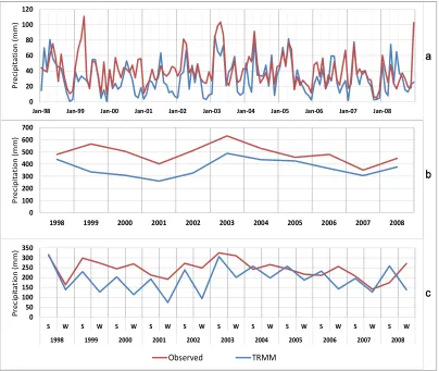
Finally, the monthly-, annually- and seasonally aggregated time series of the TRMM- rainfall
330
estimates of the average rainfall across all the studied gauge stations are plotted in Fig-5. Though
331
there is almost a persistent underestimation by the TRMM estimates, the peaks and troughs, in most
332
instances followed similar patterns.
333
334
335
Figure 5: Time series of TRMM- estimates and observed gauge data for mean rainfall totals over
336
the study area, for all the gauge stations ; a. monthly, b. annual, and c. seasonal
337
(S=Summer, W=Winter)
338
a
b
c
0 20 40 60 80 100 120
Jan-98 Jan-99 Jan-00 Jan-01 Jan-02 Jan-03 Jan-04 Jan-05 Jan-06 Jan-07 Jan-08
P
re
ci
p
it
at
io
n
(
m
m
)
0 100 200 300 400 500 600 700
1998 1999 2000 2001 2002 2003 2004 2005 2006 2007 2008
P
re
ci
p
it
at
io
n
(
m
m
)
0 50 100 150 200 250 300 350
S W S W S W S W S W S W S W S W S W S W S W
1998 1999 2000 2001 2002 2003 2004 2005 2006 2007 2008
P
re
ci
p
it
at
io
n
(
m
m
)
4.Discussions and Conclusions
339
In this study a TMPA product - TRMM 3B42 V7 data for the Upper Indus basin, Pakistan, for
340
the period 1998-2008 has been assessed and evaluated on a point-to-point basis, using rain gauge data
341
from 14 stations. These assessments have been performed at monthly, seasonal and annual
342
aggregation scales. The results indicate that the TMPA product has considerable errors in estimating
343
the rainfall amounts at the various gauge stations throughout the study area and throughout the total
344
time period studied. There is a predominant trend of under- estimation across the study area as at
345
most of the gauge stations, the TRMM product tends to under-estimate the gauge-measured rainfall,.
346
The seasonal TRMM- rainfall values, though, show a specific pattern, with the summer rainfall
347
slightly overestimated, but those for the winter predominantly underestimated at almost all locations
348
and all aggregation time scales.
349
These overall results are in conformity of the previous studies, which, in most cases, suggest that
350
neither the sparsely observed station data and gridded data products based on them, nor the sensors
351
based data, fully represent the precipitation regime of the region [41], with strong non-representation
352
or underestimation [16] of regional precipitation amounts, especially for higher altitudes by [41, 20,
353
22]. In fact the in situ meteorological observations in UIB are sparse and mostly taken at valley based
354
stations. This data provide low spatial coverage and is scant for higher altitudes. Furthermore, the
355
complex orography of the UIB region also affects the amounts, spatial patterns and seasonality of
356
precipitation. Additionally, most of the authors have indicated that the observation network across
357
the UIB, also show underestimation of precipitation amounts by [20, 22, 41–43], with an average
358
underestimation of around 166%, which may reach even in excess of 300% over some parts of the
359
basin [43]. This means that the TRMM product may even be underestimating the true areal
360
precipitation by a much greater margin, as the true areal precipitation is estimated to be much higher
361
[43] than the gauge observation records.
362
The comparison of any gridded or sensor based dataset against the observed precipitation, may
363
not be taken, therefore, as a conclusive evidence for declaring the evaluated data as unappropriated
364
in terms of usability but rather show the degree to which these data sets match for magnitudes or
365
occurrences with the observed precipitation, which by no means is perfect., and a better match may
366
also indicate the evaluated data also may have tendencies to underestimate the real areal
367
precipitation over the UIB. Furthermore, the resolution of the TRMM product (0.25° X 0.25°), may
368
also pose limitations, especially for distributed hydrological modelling and investigations, as at this
369
resolution, the orographic influences on the precipitation regime cannot be mapped, while the
370
hydrological models may also require precipitation data at a much finer scale.
371
The main conclusion which can be drawn from our study may be summed up as: 1) The TRMM
372
3B42 V7 product has an overall poor agreement with the observed rainfall gauge data in the study
373
area, and this holds for all temporal scales considered; and 2) our results, eventually means that
374
the TMPA-TRMM 3B42 V7 product may only be regarded as suitable for further rainfall analyses and
375
subsequent hydrological applications in the study region, if some improvements, down-scaling and
376
local calibrations of its output data are carried out first.
377
378
Author Contributions:
379
Asim Jahangir Khan conceived and designed the experiments, conducted the analysis and is responsible for
380
writing; Manfred Koch helped developing the idea, supervised the analyses and the writing process and he is
381
responsible for parts of the text; Karen Milena Chinchilla is responsible for parts of the statistical analysis and
382
helped developing ideas.
383
Funding: “This research received no external funding”.
384
Acknowledgments: “Tropical Rainfall Measurement Mission Project (TRMM), Daily TRMM and Others Rainfall
385
Estimate (3B42 V7 derived), version 7, data used in this study were produced with the Giovanni online data
386
system, developed and maintained by the NASA GES DISC."
387
Conflicts of Interest: “The authors declare no conflict of interest.”
388
References
390
391
1. Scheel, M.L.M.; Rohrer, M.; Huggel, C.; Santos Villar, D.; Silvestre, E.; Huffman, G.J. Evaluation of
392
TRMM Multi-satellite Precipitation Analysis (TMPA) performance in the Central Andes region and its
393
dependency on spatial and temporal resolution. Hydrol. Earth Syst. Sci. 2011, 15, 2649–2663,
394
doi:10.5194/hess-15-2649-2011.
395
2. Hasanpour Kashani, M.; Dinpashoh, Y. Evaluation of efficiency of different estimation methods for
396
missing climatological data. Stoch Environ Res Risk Assess2012, 26, 59–71,
doi:10.1007/s00477-011-397
0536-y.
398
3. Behrangi, A.; Khakbaz, B.; Jaw, T.C.; AghaKouchak, A.; Hsu, K.; Sorooshian, S. Hydrologic evaluation
399
of satellite precipitation products over a mid-size basin. Journal of Hydrology 2011, 397, 225–237,
400
doi:10.1016/j.jhydrol.2010.11.043.
401
4. Pegram, G.; Deyzel, I.; Sinclair, S.; Visser, P.; Terblanche, D.; Green, G. Daily mapping of 24 hr rainfall
402
at pixel scale over South Africa using satellite, radar and raingauge data: In: 2nd International Precipitation
403
Working Group (IPWG) Workshop, Naval Research Laboratory, Monterey, USA. 25-28 October 2004.
404
5. Ghile, Y.; Schulze, R.; Brown, C. Evaluating the performance of ground-based and remotely sensed near
405
real-time rainfall fields from a hydrological perspective. Hydrological Sciences Journal2010, 55, 497–
406
511, doi:10.1080/02626667.2010.481374.
407
6. Oke, A.M.C.; Frost, A.J.; Beesley, C.A. The use of TRMM satellite data as a predictor in the spatial
408
interpolation of daily precipitation over Australia: In: 18th World IMACS/MODSIM Congress, 13-17
409
July 2009.
410
7. Chiew FHS, Vaze J, Viney NR, Jordan PW, Perraud J-M, Zhang L, Teng J, Young WJ, Penaarancibia J,
411
Morden RA, Freebairn. Rainfall-runoff modelling across the Murray-Darling Basin. A report to the
412
Australian Government from the CSIRO Murray-Darling Basin Sustainable Yields ProjecT; CSIRO,
413
Australia, 2008.
414
8. Hughes, D.A. Comparison of satellite rainfall data with observations from gauging station networks.
415
Journal of Hydrology2006, 327, 399–410, doi:10.1016/j.jhydrol.2005.11.041.
416
9. Joyce, R.J.; Janowiak, J.E.; Arkin, P.A.; Xie, P. CMORPH: A Method that Produces Global Precipitation
417
Estimates from Passive Microwave and Infrared Data at High Spatial and Temporal Resolution. J.
418
Hydrometeor2004, 5, 487–503, doi:10.1175/1525-7541(2004)005<0487:CAMTPG>2.0.CO;2.
419
10. KUBOTA, T.; SHIGE, S.; Hashizume, H.; AONASHI, K.; TAKAHASHI, N.; Seto, S.; HIROSE, M.;
420
TAKAYABU, Y.N.; Ushio, T.; Nakagawa, K.; et al. Global Precipitation Map Using Satellite-Borne
421
Microwave Radiometers by the GSMaP Project: Production and Validation. IEEE Trans. Geosci. Remote
422
Sensing2007, 45, 2259–2275, doi:10.1109/TGRS.2007.895337.
423
11. Ushio, T.; SASASHIGE, K.; KUBOTA, T.; SHIGE, S.; Okamoto, K.'i.; AONASHI, K.; INOUE, T.;
424
TAKAHASHI, N.; IGUCHI, T.; Kachi, M.; et al. A Kalman Filter Approach to the Global Satellite
425
Mapping of Precipitation (GSMaP) from Combined Passive Microwave and Infrared Radiometric Data.
426
JMSJ2009, 87A, 137–151, doi:10.2151/jmsj.87A.137.
12. AONASHI, K.; AWAKA, J.; HIROSE, M.; KOZU, T.; KUBOTA, T.; LIU, G.; SHIGE, S.; KIDA, S.;
428
SETO, S.; TAKAHASHI, N.; et al. GSMaP Passive Microwave Precipitation Retrieval Algorithm :
429
Algorithm Description and Validation. JMSJ2009, 87A, 119–136, doi:10.2151/jmsj.87A.119.
430
13. Turk, F.J. Rohaly, G.D., Hawkins, J. Smith, E.A., Marzano, F.S. Mugnai, A. Levizzani, V. Meteorological
431
applications of precipitation estimation from combined SSM/I, TRMM and infrared geostationary satellite
432
data. In book: Microwave Radiometry and Remote Sensing of the Earth’s Surface and Atmosphere; VSP
433
Intl. Sci. Publ. Zeist, pp 353–363, 2000.
434
14. Huffman, G.J.; Adler, R.F.; Bolvin, D.T.; Nelkin, E.J. The TRMM Multi-Satellite Precipitation Analysis
435
(TMPA).: In: Gebremichael M., Hossain F. (eds) Satellite Rainfall Applications for Surface Hydrology.
436
Springer, Dordrecht 2010, 3–22, doi:10.1007/978-90-481-2915-7_1.
437
15. Huffman, G.J.; Bolvin, D.T.; Nelkin, E.J.; Wolff, D.B.; Adler, R.F.; Gu, G.; Hong, Y.; Bowman, K.P.;
438
Stocker, E.F. The TRMM Multisatellite Precipitation Analysis (TMPA): Quasi-Global, Multiyear,
439
Combined-Sensor Precipitation Estimates at Fine Scales. J. Hydrometeor 2007, 8, 38–55,
440
doi:10.1175/JHM560.1.
441
16. Andermann, C.; Bonnet, S.; Gloaguen, R. Evaluation of precipitation data sets along the Himalayan front.
442
Geochem. Geophys. Geosyst.2011, 12, n/a-n/a, doi:10.1029/2011GC003513.
443
17. Amir Khan, A.; Pant, N.C.; Ravindra, R.; Alok, A.; Gupta, M.; Gupta, S. A precipitation perspective of
444
the Hydrosphere-cryosphere interaction in the Himalaya. Geological Society, London, Special
445
Publications2018, 462, 73–87, doi:10.1144/SP462.2.
446
18. Hussain, S.; Song, X.; Ren, G.; Hussain, I.; Han, D.; Zaman, M.H. Evaluation of gridded precipitation
447
data in the Hindu Kush–Karakoram–Himalaya mountainous area. Hydrological Sciences Journal2017,
448
62, 2393–2405, doi:10.1080/02626667.2017.1384548.
449
19. Cheema, M.J.M.; Bastiaanssen, W.G.M. Local calibration of remotely sensed rainfall from the TRMM
450
satellite for different periods and spatial scales in the Indus Basin. International Journal of Remote Sensing
451
2012, 33, 2603–2627, doi:10.1080/01431161.2011.617397.
452
20. Yatagai, A.; Kamiguchi, K.; Arakawa, O.; Hamada, A.; Yasutomi, N.; Kitoh, A. APHRODITE:
453
Constructing a Long-Term Daily Gridded Precipitation Dataset for Asia Based on a Dense Network of
454
Rain Gauges. Bull. Amer. Meteor. Soc.2012, 93, 1401–1415, doi:10.1175/BAMS-D-11-00122.1.
455
21. Palazzi, E.; Filippi, L.; Hardenberg, J. von. Insights into elevation-dependent warming in the Tibetan
456
Plateau-Himalayas from CMIP5 model simulations. Clim Dyn2017, 48, 3991–4008,
doi:10.1007/s00382-457
016-3316-z.
458
22. Wijngaard, R.R.; Lutz, A.F.; Nepal, S.; Khanal, S.; Pradhananga, S.; Shrestha, A.B.; Immerzeel, W.W.
459
Future changes in hydro-climatic extremes in the Upper Indus, Ganges, and Brahmaputra River basins.
460
PLoS ONE2017, 12, e0190224, doi:10.1371/journal.pone.0190224.
461
23. Wilheit, T.T. Some Comments on Passive Microwave Measurement of Rain. Bull. Amer. Meteor. Soc.
462
1986, 67, 1226–1232, doi:10.1175/1520-0477(1986)067<1226:SCOPMM>2.0.CO;2.
463
24. Janowiak, J.E.; Joyce, R.J.; Yarosh, Y. A Real–Time Global Half–Hourly Pixel–Resolution Infrared
464
Dataset and Its Applications. Bull. Amer. Meteor. Soc. 2001, 82, 205–217,
doi:10.1175/1520-465
0477(2001)082<0205:ARTGHH>2.3.CO;2.
25. Ali, K.F.; Boer, D.H. de. Spatial patterns and variation of suspended sediment yield in the upper Indus
467
River basin, northern Pakistan. Journal of Hydrology 2007, 334, 368–387,
468
doi:10.1016/j.jhydrol.2006.10.013.
469
26. Hewitt, K. Hazards of melting as an option: Upper Indus Glaciers,I&II. DAWN, May 20, 2001.
470
27. Tahir, A.A.; Chevallier, P.; Arnaud, Y.; Neppel, L.; Ahmad, B. Modeling snowmelt-runoff under climate
471
scenarios in the Hunza River basin, Karakoram Range, Northern Pakistan. Journal of Hydrology2011,
472
409, 104–117, doi:10.1016/j.jhydrol.2011.08.035.
473
28. Immerzeel, W.W.; van Beek, L.P.H.; Bierkens, M.F.P. Climate Change Will Affect the Asian Water
474
Towers. Science2010, 328, 1382–1385, doi:10.1126/science.1183188.
475
29. Wake, C.P. Glaciochemical Investigations as a Tool for Determining the Spatial and Seasonal Variation
476
of Snow Accumulation in the Central Karakoram, Northern Pakistan. A. Glaciology.1989, 13, 279–284,
477
doi:10.3189/S0260305500008053.
478
30. Hewitt, K. Glacier Change, Concentration, and Elevation Effects in the Karakoram Himalaya, Upper
479
Indus Basin. Mountain Research and Development2011, 31, 188–200,
doi:10.1659/MRD-JOURNAL-D-480
11-00020.1.
481
31. Ali, S.; Li, D.; Congbin, F.; Khan, F. Twenty first century climatic and hydrological changes over Upper
482
Indus Basin of Himalayan region of Pakistan. Environ. Res. Lett. 2015, 10, 14007,
doi:10.1088/1748-483
9326/10/1/014007.
484
32. Hasson, S.u. Future Water Availability from Hindukush-Karakoram-Himalaya upper Indus Basin under
485
Conflicting Climate Change Scenarios. Climate2016, 4, 40, doi:10.3390/cli4030040.
486
33. Singh, P.; Kumar, N. Effect of orography on precipitation in the western Himalayan region. Journal of
487
Hydrology1997, 199, 183–206, doi:10.1016/S0022-1694(96)03222-2.
488
34. Dhar, O.N.; Rakhecha, P.R. The effect of elevation on monsoon rainfall distribution in the central
489
Himalayas. In Monsoon dynamics; Lighthill, M.J., Pearce, R.P., Eds.; Cambridge University Press: New
490
York, 1981; pp 253–260.
491
35. Dahri, Z.H.; Ludwig, F.; Moors, E.; Ahmad, B.; Khan, A.; Kabat, P. An appraisal of precipitation
492
distribution in the high-altitude catchments of the Indus basin. Science of The Total Environment2016,
493
548-549, 289–306, doi:10.1016/j.scitotenv.2016.01.001.
494
36. Pang, H.; Hou, S.; Kaspari, S.; Mayewski, P.A. Influence of regional precipitation patterns on stable
495
isotopes in ice cores from the central Himalayas. The Cryosphere2014, 8, 289–301,
doi:10.5194/tc-8-496
289-2014.
497
37. Archer, D. Contrasting hydrological regimes in the upper Indus Basin. Journal of Hydrology2003, 274,
498
198–210, doi:10.1016/S0022-1694(02)00414-6.
499
38. Mayor, Y.G.; Iryna Tereshchenko , Mariam Fonseca-Hernández; Diego A. Pantoja; Jorge M. Montes.
500
Evaluation of Error in IMERG Precipitation Estimates under Different Topographic Conditions and
501
Temporal Scales over Mexico. Remote Sensing2017, 9, 503, doi:10.3390/rs9050503.
502
39. Wilks, D.S. Statistical methods in the atmospheric sciences. An introduction; Acad. Press: San Diego,
503
1995.
40. Wilks, D.S. Statistical Methods in the Atmospheric Sciences, 3. Aufl.; Elsevier/Academic Press:
505
Amsterdam, 2011.
506
41. Palazzi, E.; Hardenberg, J. von; Provenzale, A. Precipitation in the Hindu-Kush Karakoram Himalaya:
507
Observations and future scenarios. J. Geophys. Res. Atmos. 2013, 118, 85–100,
508
doi:10.1029/2012JD018697.
509
42. Palazzi, E.; Filippi, L.; Hardenberg, J. von. Insights into elevation-dependent warming in the Tibetan
510
Plateau-Himalayas from CMIP5 model simulations. Clim Dyn2017, 48, 3991–4008,
doi:10.1007/s00382-511
016-3316-z.
512
43. Khan, A.J.; Koch, M. Correction and informed regionalization of precipitation data in a high
513
mountainous region (Upper Indus Basin) and its effect on SWAT-modelled discharge 2018 (un
514
published).