An Efficient FAST Clustering-Based Algorithm for Easy Searching

(1)

www.ijiset.com

1

An Efficient FAST Clustering-Based

Algorithm for Easy Searching

N. ShwetaP

1

P

and Dr. B. PrajnaP

2

¹-M. Tech, Department of Computer Science and Systems Engineering,

Andhra University College of Engineering, Visakhapatnam, Andhra Pradesh, India.

²-Professor, Department of Computer Science and Systems Engineering,

Andhra University College of Engineering, Visakhapatnam, Andhra Pradesh, India.

Abstract

Nowadays huge amount of high dimensional data is being used widely in different fields. These high dimensional data consist of varying features and attributes. It represents both text and image data. In order to maintain the quality and dimensionality of data, all the irrelevant and redundant features are processed and removed from the original set of data. A good feature selection algorithm selects the most appropriate features from the entire set of features so that the output obtained contains only relevant data. Different approaches for feature selection involves wrapper approach, filter approach, embedded approach and feature selection algorithm. A feature selection algorithm must be introduced so that the features are selected based on the efficiency and effectiveness of the algorithm. The time required to find a subset of features must be minimum and the quality of subset of features must be high. Based on these constraints, a novel clustering based feature subset selection algorithm for high dimensional data, Fast clustering-bAsed feature Selection algoriThm(FAST)is proposed. This algorithm works mainly in two steps. Firstly, all the available features are classified into clusters using graph-theoretic clustering methods. Next, the most appropriate feature is selected from each cluster such that it is strongly related to target classes to form a subset of features. The algorithm works by removing irrelevant features from the given dataset followed by minimum spanning tree construction and selecting the most representative features preceded by tree partitioning. In order to increase the efficiency of FAST algorithm, MST clustering method is adopted. The effectiveness of the algorithm is evaluated through comparative study of FAST with several representative feature selection algorithms such as FCBF, ReliefF, CFS, Consist and FOCUS-SF.

Keywords: Feature subset selection, feature

clustering, relevance, redundancy, feature selection methods.

1. INTRODUCTION

Feature subset selection is important with the aim of selecting a subset of good features with respect to the target concepts. This helps reduce the dimensionality of the data, removes irrelevant and redundant data, hence increasing learning accuracy and improving result quality [18], [19]. Different feature subset selection methods have been proposed namely, the Embedded, Wrapper, Filter and Hybrid approaches.

A. Wrapper approach for feature selection

(2)

www.ijiset.com

2

test data sets, the induction algorithm run n times.

The results obtained in each run are combined together to obtain the accuracy. Feature space is searched for finding better features. For finding better features, algorithms like forward selection, backward elimination etc are used. The

working of forward and backward algorithms is similar with only difference in the selection of

features. The backward algorithm begins with all features whereas forward algorithm begins with no

features. The wrappers use cross validation measures of predictive accuracy to avoid over fitting and hence acquire the ability of generality.

Figure 1. Wrapper approach to feature subset selection [20]

Figure 1 shows an induction algorithm based on wrapper approach. The algorithm is treated as black box. There are two partitions in the algorithm namely the training sets and the hold out sets. The feature subset selection algorithm acts as a wrapper around the induction algorithm. It conducts search

for better subsets using induction algorithm itself as a part of function evaluating feature subsets. The algorithm removes several feature sets from the dataset. The induction algorithm runs on those feature subsets with highest evaluation and the final classifier is evaluated.

Figure 2. The filter approach to feature selection [8].

Input Features

Feature Subset

Selection

(3)

www.ijiset.com

208 B. Filter approach for feature selection

I. Guyon and A.Elisse proposed filter methods for feature selection [8], [5]. Filter methods can be further divided into univariate and multivariate. In univariate technique, the filter model considers only one feature at a time, while the multivariate techniques consider subset features together, aiming at incorporating feature.

Figure 2 shows the feature filter approach, in which the features are filtered independently of the induction algorithm. Filter approaches are pre-selection methods that are independent of the machine learning algorithm. It selects features after performing pre-processing. The main drawback of the filter approach is that it totally overlooks the impacts of the selected feature subset on the performance of the induction algorithm. Several algorithms are used in filter selection methods. They are Focus algorithm, Relief algorithm, decision trees, etc. Focus Algorithm is one of the algorithms which use the filter method. This algorithm is defined for noise-free Boolean domains. It selects minimal feature subsets which determine the values for labels from the data set. This is referred to as MIN-FEATURES bias. i.e., this algorithm searches for minimum features. Arauzo and Azofra proposed a feature selection algorithm based on attribute estimation known as relief algorithm [8], [9]. The Relief algorithm is a randomized algorithm which finds relevance of feature to target concept by assigning a relevance value to each feature. It randomly selects the instances from the training set and updates the relevance values in view of the difference between the selected instance and the two nearest instances of the similar and dissimilar classes (the “near-hit” and “near-miss”). The Relief algorithm aims at finding all the useful and necessary features from the subset of features. It does not help with redundant features. If most of the given features are relevant to the concept, it would select most of them even though only a fraction is necessary for concept description. In real time applications, multiple features have a strong interdependency with the label, hence this type of features are weakly relevant and are difficult to get rid of by the Relief. The extended Relief algorithm [10] is motivated by nearest-neighbours and it is good specifically for similar types of induction algorithms. Since Relief randomly samples instances and their neighbours from the training set, the answers it gives are unreliable without a large number of samples.

C. Embedded approach for feature selection

Al Blum and P Langley proposed embedded approach for feature selection. It is also known as

nested subset method [11]. Figure 3 describes the steps for obtaining features from training data using some classifier and optimization techniques. During the classification process, the algorithm decides which attributes to use and which to ignore. Just like wrapper methods, an embedded approach depends on a specific learning algorithm. Decision trees are examples of embedded approaches. This algorithm evaluates feature subsets with the classification algorithm to measure efficiency according to incorrect classification rate. It uses an algorithm known as Sequential Forward Selection (SFS). The computational complexity is higher than one of filter methods but selected subsets are more efficient. SFS begins with empty subset of features. The new subset with features is obtained by adding a single new feature to the subset which performs best among remaining features.

Figure 3. Embedded approach for feature selection [7]

The correct classification rate is obtained by the selected feature subset. In each step of algorithm, a threshold is set according to the compromise between the performance and computational burden. All subsets with performance above a threshold are kept to enter the evaluation in the next step. Features thus selected have the ability to discriminate among classes that occur in training data are further used. The classifier used here is based on belief masses of features which are modelled from distribution of features for each class obtained from the training data.

D. Feature subset selection algorithm

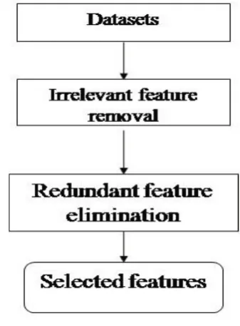
Feature subset selection can distinguish noisy and redundant information. Good feature subsets can be derived in a cost-effective manner using feature selection algorithms [12]. Figure 4 consists of two linked components of irrelevant feature removal and redundant feature elimination. The first one selects features based on a target class by removing irrelevant ones and the second one removes redundant features from relevant one by selecting

Internal Optimizatio

n Classifier

Decision Rule

+

Selected Features Training

(4)

www.ijiset.com

209

samples from different clusters of features and then

creates the final subset. A feature selection algorithm is evaluated from two views namely, efficiency and effectiveness. Efficiency is related to the time required to find a subset of features and the effectiveness is related to the quality of the subset of features.

.

Figure 4. Feature subset selection algorithm

Based on these norms, a fast clustering-based feature selection algorithm, FAST is proposed The FAST algorithm, first divides the features into clusters by using graph-theoretic clustering methods [13]. In the second step, the most typical feature that is strongly related to target classes is selected from each cluster and forms feature subsets. Features in each cluster are relatively independent. The clustering-based procedure of FAST has a high probability of generating a subset of useful and independent features. To ensure the efficiency of FAST, an efficient minimum-spanning tree (MST) clustering methods are adopted. In this paper, the efficiency and effectiveness of the FAST algorithm is improved and enhanced algorithms are been used.

In the FAST algorithm, relevant features are represented in the form of a tree called Minimum Spanning Tree(MST) where all the necessary and relevant features are denoted as the nodes of a tree. The clustering is performed in such a way that the algorithm takes less time and more accuracy in finding the subset of features. The proposed feature selection algorithm is been tested using 35 publicly available datasets consisting of collection of images, microarray and text data sets. The obtained results are compared with other feature selection algorithms. The algorithm not only increases the performance while searching but also reduces the

time taken for feature subset selection. The rest of the article is organized as follows: Section 2 explains the problems with the already existing feature subset selection algorithm. Section 3 proposes the new feature selection algorithm. In Section 4 , methods for implementing the efficient FAST is discussed. In Section 5, analysis is performed based on the experimental results obtained to support the proposed FAST algorithm. Section 6 summarizes the present work and concludes the paper.

2. PROBLEM STATEMENT

The embedded methods incorporate feature selection as a part of the training process and are usually specific to given learning algorithms, and therefore may be more efficient than the other three categories. Some of the machines learning algorithms like decision trees or artificial neural networks are examples of embedded approaches. In the wrapper methods, the goodness of the selected subsets is determined using the predictive accuracy of a predetermined learning algorithm and the accuracy of the learning algorithms is usually high. However, the generality of the selected features is limited and the computational complexity is large.

The filter methods do not depend on learning algorithms, with good generality. It takes less time for computation but the accuracy of the learning algorithms is not predictable. The hybrid methods are a combination of filter and wrapper methods by using a filter method to reduce search space that will be considered by the subsequent wrapper [21]. The main aim is to combine filter and wrapper methods in order to achieve the best possible performance using a particular learning algorithm having same time complexity as that of the filter methods.

2.1 Disadvantages

a. 18TThe generality of the selected features is limited and the time taken for computation is large.

b. 19TTheir computational complexity is low, but the accuracy of the learning algorithms cannot be predicted.

3. PROPOSED SYSTEM

(5)

www.ijiset.com

210

algorithm can eliminate irrelevant features along

with handling redundant features. Some of the feature subset selection algorithms mainly focuses on searching for relevant features, for example, Relief algorithm. It selects each feature based on its ability to differentiate between instances under different targets based on distance-based criteria function. However, Relief is unable to remove redundant features as the highly correlated features are likely both to be highly weighted. Further the enhanced part of Relief was used namely Relief-F which can remove noisy and unnecessary datasets and also deals with multiclass problems but is unable to remove redundant features.

i. 19TGood feature subsets contain features that are highly correlated with (predictive of) the class, yet uncorrelated with each other. ii. 19TThe efficiency and effectiveness of the

algorithm depends on both irrelevant and redundant features to obtain a good feature subset.

3.1 Framework and definition

In order to more precisely introduce the algorithm, and because our proposed feature subset selection framework involves irrelevant feature removal and redundant feature elimination [1], we firstly present the traditional definitions of relevant and redundant features, then provide our definition based on variable correlation as follows. Suppose F to be the full set of features, FRi Rϵ F be a feature, Sᵢ=F-{Fᵢ} and S'ᵢ ϹSᵢ. Let s’ᵢ be a value-assignment of the target concept C. The definitions can be framed as follows.

Definition 1: (Relevant feature) Fᵢ is relevant to

the target concept C if and only if there exists some s’ᵢ, fᵢ and c, such that, for probability p (S'ᵢ=s'ᵢ, Fᵢ=fᵢ)>0, p (C=c|S'ᵢ=s’ᵢ, Fᵢ=fᵢ) ≠p (C=c |S'ᵢ=s'ᵢ). Otherwise, feature Fᵢ is an irrelevant feature. Definition 1 indicates that there are two kinds of relevant features due to different S'ᵢ: (i) when S'ᵢ=Sᵢ, from the definition we can know that Fᵢ is directly relevant to the target concept; (ii) when S'ᵢ Ϲ Sᵢ, from the definition we may obtain that p (C| Sᵢ, Fᵢ) =p(C|Sᵢ). It seems that Fᵢ is irrelevant to the target concept. However, the definition shows that feature Fᵢ is relevant when using S'ᵢ ᴜ {Fᵢ} to describe the target concept. The reason behind is that either Fᵢ is interactive with S'ᵢ or Fᵢ is redundant with Sᵢ–S'ᵢ. In this case, we say Fᵢ is indirectly relevant to the target concept.

Redundant features provide a poor interpreting ability to the target concept. As most of the information obtained from the redundant features is already present in the other features.

Definition 2: (Markov blanket) Given a feature Fᵢ

ϵ F, let Mᵢ Ϲ F (Fᵢ ¢ Mᵢ) is said to be Markov blanket for Fᵢ if and only if

P (F – Mᵢ – {Fᵢ}, C | Fᵢ, Mᵢ) =p (F – Mᵢ – {Fᵢ}, C| Mᵢ).

Definition 3:(Redundant feature) Assume that S

be a set of features, a feature in S is said to be redundant if and only if it has a Markov Blanket within S.

Relevant features have strong correlation with target concept whereas redundant features are not because their values are completely correlated with each other. Hence, feature redundancy and feature relevance are normally demonstrated in terms of feature correlation and feature-target concept correlation.

Mutual information measures how much the distribution of the feature values and target classes differ from statistical independence. This is a non-linear estimation of correlation between feature values or feature values and target classes. The symmetric uncertainty (SU) [14] is derived from the mutual information by normalizing it to the entropies of feature values or feature values and target classes, and has been used to evaluate the goodness of features for classification by a number of researchers [3,14]. Therefore, symmetric uncertainty is chosen as the measure of correlation between either two features or a feature and the target concept.

The symmetric uncertainty is defined as follows

SU(X, Y) = _{H(X) + H(Y)}2∗Gain(X|Y) (1)

Where,

• H(X) is the entropy of a discrete random variable X. Consider p(x) as the prior probabilities for all values of X, H(X) is defined by

𝐻(𝑋) =− � 𝑝(𝑥)𝑙𝑜𝑔2𝑝(𝑥) (2) 𝑥𝜖𝑋

• Gain (X|Y) is the amount by which the entropy of Y decreases. It reflects the additional information about Y provided by X and is called the information gain [16]is given by

𝐺𝑎𝑖𝑛(𝑋|𝑌) =𝐻(𝑋)− 𝐻(𝑋|𝑌)

=𝐻(𝑌)− 𝐻(𝑌|𝑋) (3)

Where,

(6)

www.ijiset.com

211

posterior probabilities of X given the values of Y,

H(X|Y) is defined by

𝐻(𝑋|𝑌) =− � 𝑝(𝑦)

𝑦𝜖𝑌

� 𝑝(𝑥|𝑦)𝑙𝑜𝑔2𝑝(𝑥|𝑦) (4) 𝑥𝜖𝑋

Information gain is a symmetrical measure i.e., the amount of information gained about X after observing Y is equal to the amount of information gained about Y after observing X. This ensures that the order of two variables (e.g., (X, Y) or (Y, X)) will not affect the value of the measure.

Symmetric uncertainty compensates for information gain’s bias toward variables with more values and normalizes its value to the range [0,1]. If SU (X, Y) value is 1 indicates that knowledge of the value of either one completely predicts the value of the other whereas the value 0 reveals that X and Y are independent. Although the entropy based measure handles nominal or discrete variables, they can deal with continuous features as well, if the values are discretized properly in advance [17].

Given SU (X, Y) the symmetric uncertainty of variables X and Y, the relevance T-relevance

between a feature and the target concept C. The correlation F-Correlation between a pair of features, the feature redundancy F-Redundancy and the representative feature R-Feature of a feature cluster can be defined as follows.

Definition 4: (T-Relevance) T-Relevance of the

feature Fᵢ and the target concept C is defined as the relevance between the feature Fᵢ ϵ F and the target concept C, and denoted by SU (Fᵢ, C).

If SU (Fᵢ,C) is greater than a predetermined threshold θ, we say that Fᵢ is a strong T-Relevance feature.

Definition 5: (F-Correlation) The correlation

between any pair of features Fᵢ and F ⱼ (Fᵢ, F ⱼϵ FɅ i ≠j) is called the F-Correlation of Fᵢ and F ⱼ, and denoted by SU (Fᵢ, F ⱼ).

Definition6:(F-Redundancy) Let

𝑆= {𝐹𝐹1,𝐹𝐹2,….,𝐹𝐹𝑖, … ,𝐹𝐹𝑘<|𝐹|}

be a cluster of features. If ⱼ Fⱼ ϵ S, SU (F ⱼ, C) ≥ SU (Fᵢ, C) Ʌ SU (Fᵢ, F ⱼ)> SU (Fᵢ, C) is always corrected for each Fᵢ ϵ S (i ≠j), then Fᵢ are redundant features with respect to the given F ⱼ (i.e. each Fᵢ is a F-Redundancy).

Definition 7: (R-Feature) A Feature Fᵢ ϵ S= {F1,

F2…., Fk} (k<|F|) is a representative feature of the cluster S (i.e. Fᵢ is a R-Feature) if and only if,

𝐹𝐹ᵢ=𝑎𝑟𝑔𝑚𝑎𝑥𝐹ᵢ𝜖𝑆𝑆𝑈(𝐹𝐹�,𝐶)

This means the feature, which has the strongest T-Relevance, can act as a R-Feature for all the features in the cluster.

According to the above definitions, feature subset selection can be the process that identifies and retains the strong T-relevance features and selects R-Features from feature clusters. The behind heuristics are that

• irrelevant features have no or weak correlation with target concept;

• redundant features are assembled in a cluster and a representative feature can be taken out of the cluster.

3.2 Algorithm and Analysis

The proposed FAST algorithm logically consists of three steps: (i) removing irrelevant features, (ii) constructing a MST from relative ones, and (iii) partitioning the MST and selecting representative features.

For a data set D with m features F = {FR1R, FR2R, ...FRmR}and class C, we compute the T-Relevance SU (FRiR, C) value for each feature FRiR(1 ≤ i ≤ m) in the first step. The features whose SU (FRiR, C) values are greater than a predefined threshold Ø comprise the target-relevant feature subset FP

'

P

= {FP

'

PR1R, FP

'

PR2, ...R FP

'

PRkR} (k≤m).

In the second step, we first calculate the F-Correlation SU(FP

'

P

ᵢ,F'RjR) value for each pair of features FP

'

P

ᵢ and F'RjR(FP

'

P

ᵢ, F'RjR) value for each pair of features FP

'

P

ᵢand F'Rj Ras vertices and SU(FP

'

P

ᵢ,F'RjR) (i ≠ j) as the weight of the edge between vertices FP

'

P

ᵢ and FP

'

P

j, a weighted complete graph G=(V, E)is constructed where V = { FP

'

P

ᵢ│F'RjRϵ FP

'

P

ⱼ i ϵ [1,k]} and E={(FP

'

P

ᵢ,F'RjR) │ (FP

'

P

ᵢ,F'RjRϵ FP

'

P

ⱼ i, j ϵ [1, k] ⱼ i ≠ j}. As symmetric uncertainty is symmetric further the

F-Correlation SU (FP

’ᵢ, F’j

P

) is symmetric as well, thus G is an undirected graph.

The complete graph G reflects the correlations among all the target-relevant features. Unfortunately, graph G has k vertices and k(k-1)/2 edges. For high dimensional data, it is heavily dense and the edges with different weights are strongly interweaved. Moreover, the decomposition of complete graph is NP-hard. Thus, for graph G, we build as MST, which connects all vertices such that the sum of the weights of the edges is the minimum, using the well-known as Kruskal’s algorithm. The weight of edges (FP

'

P

ᵢ, F'RjR) is F-Correlation SU (FP

'

P

ᵢ, F'RjR).

After building the MST, in the third step, we first remove the edges E= {(FP

'

P

ᵢ, F'RjR) │ (FP

’ᵢ, F’j

P

ϵ FP

'

P

ⱼ i, j ϵ

[i, k] ⱼ i ≠ j}, whose w

of the T-Relevance SU (FP

'

P

(7)

www.ijiset.com

212

Assuming the set of vertices in any one of the final

trees to be V(T), we have the property that for each pair of vertices (FP

’ᵢ, F’j

Pε V(T)), SU (FP

’ᵢ, F’j

P

) ≥ SU (FP

'

P

ᵢ, C) V SU (FP

'

P

ᵢ, F'RjR) ≥ SU (F'RjR, C) always guarantees the features in V(T) are redundant.

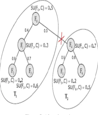
This can be illustrated by an example. Suppose the MST is generated from a complete graph G as shown in Figure 5. In order to cluster the features, we first traverse all the six edges, and the decide to remove the edge (FR0, RFR4R) because its weight SU (FR0R, FR4R) because its weight SU (FR0R, FR4R) = 0.3 is smaller than both SU (FR0, RC) =0.5 and SU (FR4,R C) =0.7. This makes the MST is clustered into two clusters denoted as V(TR1R) and V(TR2R). Each cluster is a MST as well. Take V(TR1R) as an example. We know that SU (FR0, RFR1R) > SU (FR1, RC), SU (FR1, RFR2R)> SU (FR1, RC) ɅSU (FR1, RFR2R) > SU (FR2, RC), SU (FR1, RFR3R) > SU (FR1, RC) Ʌ SU (FR1, RFR3R) > SU (FR3, RC). We also observed that there is no edge exists between FR0R and FR2R,FR0R and FR3R,and FR2R and FR3R.Considering that TR1R is a MST, so that SU(FR0R,FR2R) is greater that SU(FR0R,FR1R) and SU(FR1R,FR2R),SU(FR0R,FR3R)is greater than SU(FR0R,FR1R) and SU(FR1R,FR3R) ,and SU(FR2R,FR3R)is greater than SU(FR1R,FR2R) and SU(FR2R,FR3R).Thus ,SU(FR0R,FR2R) > SU(FR0R,C) Ʌ SU(FR0R,FR2R) > SU(FR2R,C), SU(FR0R,FR3R) > SU(FR0R,C) Ʌ SU(FR0R,FR3R) > SU(FR3R,C), and SU(FR2R,FR3R) > SU(FR2R,C) Ʌ SU(FR2R,FR3R) > SU(FR3R,C) also hold. As the mutual information between any pair (FRiR, Fj) (i, j=0,1,2,3Ʌi≠j) of FR0R, FR1R, FR2R, and FR3R is greater than the mutual information between class C and FRiR or Fj, features FR0R, FR1R, FR2R, and FR3R are redundant.

Figure 5: After clustering

After removing all the unnecessary edges from the graph, a Forest is obtained. Each tree TRjR ϵ Forest represents a cluster that is denoted as V(TRjR), which is the vertex set of TRjR as well. As illustrated above, the features in each cluster are redundant, so for each cluster V(TRjR) we choose a representative feature FRRRP

i

P

whose T-Relevance SU (FRRRP

i

P

, C) is the

greatest. All FRRRP

j

P(j = 1...│Forest│) comprise the final feature subset ᴜ FRRRP

j

P

. The details of the FAST algorithm are shown in Algorithm 1.

Algorithm 1: FAST

Inputs: the given dataset D (F1, F2…., Fm, C) θ the T-Relevance threshold

Output: S-the selected feature subset //Part 1 Irrelevant feature removal for i= 1 to m do

T-Relevance=SU (Fi, C) if T-Relevance>θ then

S=S ᴜ{Fi};

//Part 2 Minimum spanning tree construction G=NULL; where G is a complete graph for each pair of features {F'i, F'j} Ϲ S do

F-Correlation = SU (F’i, F’j)

Add features F'i and/or F'j to G using F-Correlation as the weight of the corresponding edge;

minSpanTree=Prim(G);

//Part 3 Tree partitioning and Representative feature selection

Forest=minSpanTree for each edge Eij ϵ Forest do

if SU (F’i, F’j) < SU (F'i,C) Ʌ SU (F’i, F’j) < SU (F'i,C) then

Forest=Forest – Eij S=Ø

for each tree TRiRϵ Forest do

𝐹𝐹ᴶ 𝑅𝑅=argmax F'k ϵ TRiR SU (F’k,C) S=S ᴜ {𝐹𝐹ᴶ 𝑅𝑅};

return S

Kruskal’s algorithm is a greedy algorithm that creates a minimum spanning tree for a connected weighted graph. It finds shortest path which a subset of edges such that every vertex of the tree is visited and total weight of all the edges is minimized. If the graph is not connected then it finds a minimum spanning forest (i.e. a minimum spanning tree for each connected component). The steps involved in Kruskal’s algorithm is explained in Algorithm 2.

Algorithm2:

MST_Kruskal () begin

Input: simple connected graph represented by array of edges, represented by edge []

Output: list of edges T in MST

// Create a partition for the set of vertices foreach vertex v ϵ V

Cv: = {v}

// create a minHeap h using the array of edges E h: = new Heap(E)

(8)

www.ijiset.com

213

while size(T) < n-1

(u, v, wgt): =h. removeMin () Cv: = findSet(v)

Cu: = findSet(u) if Cu ≠ Cv union (Cu, Cv) T: = T ᴜ {(u, v, wgt)} return T

end

The above algorithm creates a minimum spanning tree from a connected weighted graph. Cu, Cv are the root vertex of tree each representing disjoint set of vertices.

findSet () operation: first find which sets the edge

vertices belong to.

union () operation: If the vertex sets are disjoint,

the edge is added to the MST and the union of the two sets is obtained.

All the edges of the graph are grouped into a set namely S while S is nonempty and T (a set of trees, where each vertex in the graph is a separate tree) is not yet spanning.

• remove an edge having minimum weight from

S

• if that edge contains more than one connected trees then add it to the forest combining it into a single tree, otherwise discard that edge.

At the end of the algorithm, T has only one component and forms a minimum spanning tree of the graph.

4. METHODOLOGY

Implementation involves applying the theoretical design into a working system using different methods. It is the most important stage in the project where the effectiveness and efficiency of the work is being decided. It involves study of the existing system and its constraints on implementation, and evaluation of designing of proposed system.

4.1 Main Modules

4.1.1 User Module

In this module, the users are authenticated and security is provided using access control to the users. Before accessing or searching the details, user must create account in that otherwise they should register to it.

4.1.2 Distributed Clustering

The distributional clustering is used to cluster words into groups based on their particular grammatical relations (by Pereira et al.) or on the distribution of class labels associated with each

word (by Baker and McCallum). Distributional clustering of words is agglomerative in nature resulting in suboptimal clusters and has high computational cost. A new information-theoretic divisive algorithm for word clustering is proposed along with text classification. Different cluster of features are created using a special metric of distance based on which cluster hierarchy is obtained in order to choose the most relevant attributes. The main drawback with cluster evaluation measure is that distance does not identify a feature subset to improve their original performance accuracy. The accuracy obtained is lower when compared with other feature selection methods.

20T

4.1.3 Subset Selection Algorithm

The presence of irrelevant and redundant features affects the accuracy of the learning algorithms. Hence a feature subset selection algorithm must be able to remove unnecessary datasets and redundant features which is already present in other features. Finally, a subset selection algorithm must work efficiently and effectively in order to obtain a good feature subset.

20T

Time Complexity: 20TThe time complexity of

Algorithm 1 is determined in terms of number of instances in a given dataset. It involves computation of SU values for TR Relevance and F-Correlation. Suppose that the linear complexity of the first part of the algorithm in terms of the number of features is m. Assume that relevant features are selected in the first part, when k ¼ only one feature is selected.

5. EXPERMENTAL RESULTS

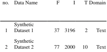
The FAST algorithm is analysed and evaluated using 20 datasets. The dataset consists of text data, images and microarray and biological data. The below Table 1 shows the characteristics of each dataset such as the number of images, type of text in each data.

TABLE 1: Summary of the 20 benchmark data sets

S.

no. Data Name F I T Domain

1

Synthetic

Dataset 1 37 3196 2 Text

2

Synthetic

(9)

www.ijiset.com

214

3

Synthetic

4

Synthetic

5

Synthetic

6

Synthetic

7

Synthetic

8

Synthetic

9

Synthetic

10

Synthetic

11

Synthetic

Dataset 11 3183 1003 10 Text

12

Synthetic

Dataset 12 3239 1050 10 Text

13

Synthetic

14

Synthetic

15

Synthetic

16

Synthetic

17

Synthetic

18

Synthetic

19

Synthetic

20

Synthetic

Clustering is performed on the above data. Features are selected by eliminating all the irrelevant and redundant features. Amongst them the most representative feature is been selected. The proposed algorithm, Kruskal’s algorithm is used where minimum spanning tree is constructed so as to make traversing of features easy. The results are displayed in tabular form where the accuracy for FAST algorithm to search and form clusters of features is compared with that of other feature selection algorithms as shown in Table 2.

TABLE 2: Accuracy of C4.5 with other feature selection algorithms

Dataset

FAST

CFS

RelieF

Synthetic Dataset 1

93.09 95.12 97.09

Synthetic Dataset 2

90.41 90.48 93.44

Synthetic Dataset 3

93.48 91.54 90.45

Synthetic Dataset 4

92.35 92.35 92.35

Synthetic Dataset 5

91.57 98.33 91.57

Synthetic Dataset 6

89.07 89.04 89.56

Synthetic Dataset 7

93.05 93.21 98.41

Synthetic Dataset 8

91.99 90.14 96.23

Synthetic Dataset 9

93.37 98.54 96.02

Synthetic Dataset 10

90.88 90.88 90.88

88.14 88.57 88.01

92.05 92.11 92.05

91.33 96.27 95.67

93.44 93.44 91.28

90.27 96.18 91.59

92.73 90.75 95.43

93.49 94.17 93.49

91.77 97.35 91.77

90.61 92.08 94.79

(10)

www.ijiset.com

215 6. CONCLUSION

In this paper, the novel clustering-based feature subset selection algorithm for high dimensional data is explained. This algorithm works in two steps-removal of irrelevant features from the dataset and selecting the most appropriate feature from the relative ones. It is achieved by constructing minimum spanning tree using Kruskal’s algorithm, partitioning the MST and selecting the representative features among the nodes. In MST, each individual tree represents a cluster and each and every cluster represents the subset of features. After clustering, results are calculated and compared with other feature selection algorithms such as FCBF, CFS, ReliefF, Consist and FOCUS-SF. The FAST algorithm ranks 1 in terms of accuracy.

7. REFERENCES

[1] Qinbao Song, Jingjie Ni and Guangtao Wang “A fast clustering-based feature subset selection algorithm for high-dimensional data” IEEE Transactions on knowledge and data engineering vol:25 no:1 ,2013.

[2]International Conference on Circuit, Power and Computing Technologies ICCPCT”Survey on Feature Subset Selection for High Dimensional Data” 2016.

[3] Hall M.A., Correlation-Based Feature Subset Selection for Machine Learning,Ph.D. dissertation Waikato, New Zealand: Univ. Waikato, 1999. [4] D.H.Fisher, L.Xu and N.Zard, “Ordering Effects in Clustering,” Proc.Ninth Int’l Workshop Machine Learning, pp. 162-168, 1992.

[5] E.Xing,M.Jordan, and R.Karp.”Feature Selection for High-dimensional Genomic Microarray Data,”Proc.18th Int’l Conf.Machine Learning,pp.601-608,2001.

[6] P.Chanda,Y.Cho,A.Zhang, and

M.Ramanathan,”Mining of Attributes Interactions Using Information Theoretic metrics,”Proc.IEEE Int’l Conf. Data Mining Workshops,pp.350-355,2009.

[7] I.Guyon and A.Elisseeff,”An Introduction to variable and Feature selection,” J Machine Learning Research,vo3,p.1157-1182,2003.

[8] A.Arauzo-Azofra, J.M.Benitez and J.L.Castro, “A Feature Set Measure Based on Relief,” Proc. Fifth Int’l Conf. Recent Advances in Soft Computing, pp. 104-109, 2004.

[9] J. Biesiada and W. Duch, “Features Election for High-Dimensional data a Pearson Redundancy Based Filter,” Advances in Soft Computing, vol.45, pp. 242-249, 2008.

[10] H. Park and H. Kwon, “Extended Relief Algorithms in Instance-Based Feature Filtering,” Proc. Sixth Int’l Conf. Advanced Language Processing and Web Information Technology (ALPIT ’07), pp. 123-128,2007.

[11] P.Langley, “Selection of Relevant Features in Machine Learning,” Proc. AAAI Fall Symp. Relevance, pp. 1-5, 1994.

[12] M.A.Hall and L.A.Smith, “Feature Selection for Machine Learning: Comparing a Correlation-Based Filter Approach to the Wrapper,” Proc. 12th Int’l Florida Artificial Intelligence Research Soc. Conf., pp. 235-239, 1999.

[13] H.Almuallim and T.G.Dietterich, “Algorithms for Identifying Relevant Features,” Proc. Ninth Canadian Conf. Artificial Intelligence, pp. 38-45, 1992.

[14] Zhao Z. and Liu H., Searching for interacting features, In Proceedings of the 20th International Joint Conference on AI, 2007.

[15] Press W.H., Flannery B.P., Teukolsky S.A. and Vetterling W.T., Numerical recipes in C. Cambridge University Press, Cambridge, 1988. [16] Quinlan J.R., C4.5: Programs for Machine Learning. San Mateo, Calif:Morgan Kaufman, 1993.

[17] Fayyad U. and Irani K., Multi-interval discretization of continuous-valued attributes for classification learning, In Proceedings of the Thirteenth International Joint Conference on Artificial Intelligence, pp 1022-1027, 1993.

[18] Liu H., Motoda H. and Yu L., Selective sampling approach to active feature selection, Artif. Intell., 159(1-2), pp 49-74 (2004).

[19] Molina L.C., Belanche L. and Nebot A., Feature selection algorithms: A survey and experimental evaluation, in Proc. IEEE Int. Conf. Data Mining, pp 306-313, 2002.

[20] R.Kohavi and G.H.John, “Wrappers for Feature Subset Selection,”Artificial Intelligence, vol. 97, nos. 1/2, pp. 273-324, 1997.

[21] L.C. Molina, L. Belanche, and A. Nebot, “Feature