SOME PRACTICAL ISSUES IN THE DESIGN AND
ANALYSIS OF COMPUTER EXPERIMENTS
Ton\- Sahama
THIS THESIS IS PRESENTED IN FULFILMENT OF
THE REQUIREMENTS OF THE DEGREE OF
DOCTOR OF PHILOSOPHY
SCHOOL O F C O M P U T E R SCIENCE AND MATHEMATICS
FACULTY O F S C I E N C E , E N G I N E E R I N G AND T E C H N O L O G Y
V I C T O R I A U N I V E R S I T Y O F T E C H N O L O G Y
FTS THESIS
519.57 SAH
30001007907837
Sahama, Tony
Some practical issues in the
design and analysis of
computer experiments
© Copyright 2003
by
Tonv Sahama
The author herelj>' grants to Victoria Universit>' of Technology permission to reproduce and distribute copies of this thesis
document in \\4iole or in part.
Certificate of Originality
I hereb\' declare that this submission is nn' own work and that, to the best of m>- knowledge and beUef, it contains no material previously pubUshed or written by another person nor material which to a substantial extent has been accepted for the award of any other degree or diploma of a universit\- or other institute of higher learning, except where due acknowledgement is made in the text.
I also hereb>- declare that this thesis is written in accordance with the Uni-versit\-'s Polic\' witli respect to the Use of Project Reports and Higher Degree Theses.
T. Sahama
Abstract
Deterministic computer simulations of physical experiments are now common techniques in science and engineering. Often, physical experiments are too time consuming, expensi\'e or impossible to conduct. Complex computer models or codes, rather than physical experiments lead to the stud>- of computer experi-ments, which are used to investigate man>' scientific phenomena of this nature. A conrputer experiment consists of a number of runs of the computer code with different input choices. The Design and Anal>-sis of Computer Experiments is a rapidly growing technique in statistical experimental design.
This thesis investigates some practical issues in the Design and Analysis of Computer experiments and attempts to answer some of the questions faced b>' experimenters using computer experiments. In particular, the cjuestion of the number of computer experiments and how tlie>- should be augmented is studied and attention is gi\'en to when the response is a function over time.
In\-estigation of the appropriate sample size for computer experiments is un-dertaken using three fire models and one circuit simulation model for empirical \-aH(lation. Detailed illustrations and some guidelines are given for the sample size and an empirical relationship is established showing how the a\'erage prediction error from a computer experiment is related to the sample size.
When tlie average prediction error following a computer experiment is too large the question of how to augment the computer experiment is raised. Two approaches are studied, e\'aluated and compared. The first approach invoh'es adding one point at a time and choosing that point with the maximum predicted \'ariance, \\4iile the second approach im'oh'es maximising the determinant of the variarice-co\'ariaiice matrix of the prediction errors of a candidate set.
Rath(>r than just examining a whole series of practical cases, the machinery of computer experiments is also used to stud>- computer experiments themseh'es. The inputs of the model are the parameters of the Krigmg model as well as the number of input runs while the output is a measure of the prediction error. This study provides predictions of the average prediction error for a wide range of computer models.
A c k n o w l e d g e m e n t s
• 1 wish to express my sincere gratitude to m>- supervisor. Dr. Neil Dia-mond, for his guidance, constructive criticism, \'aluable genuine ad\'ice and encouragement given throughout the period of m>' Ph.D. stud>' at Victoria University, Melbourne.
• I also wish to extend m>- deepest appreciation to Assoc. Prof. Neil Barnet. former Head of the School, for providing me with a departmental scholarship for the successful completion of this stud\-.
• Thanks are also rendered to Mr. P. Rajendran, Damon Burgess. Rowan Macintosh and other colleagues who ha\'e been of immense assistance through-out this stu(l>'.
• I also would like to record m>- grateful thanks to Mr. Da\'id Abercrombie and Mr. Ken Ling, School of Information S>-stems. Faculty of Information Teclmology, Queensland Uni\'ersity of Technology for their encouragement and support in numerous wa\'s.
• Special thanks to m\' wife Charlotte and our children Ishani and Ishara for gi\-ing me all the support throughout my studies.
Dedication
To my parents who taught me to work hard, to Charlotte who guided me to be fair and stay curious, and to Ishani and Ishara for keeping me honest.
Preface
Parts of Chapters 3 and 4 appeared in Sahama and Diamond (2001).
Contents
1 I n t r o d u c t i o n 1
1.1 Computer Experiments 1
1.2 Role of Experimental Designs in DACE 3 1.3 Differences between Computer Experiments and Other
Experimen-tal Design 3 1.4 Designs for Computer Experiments 5
1.5 Analysis of Computer Experiments 8
1.6 Thesis OutHne 15
2 Analysis of a Simple C o m p u t e r M o d e l 17
2.1 Introduction 17 2.2 Deterministic Fire Models 18
2.2.1 The ASET-B Fire Model 18
2.3 Experimental Design 21 2.3.1 Latin H>-perciibe Designs 21
2.3.2 Application to ASET-B Computer Experiment 22
2.4 Modelling 24 2.4.1 Summary of the Approach used by Sacks et al 24
2.4.2 Maximum Likelihood Estimation 24 2.4.-3 AppHcation to ASET-B Computer Experiment 28
2.5 Prediction 29 2.5.1 Prediction for Untried Inputs 29
2.5.2 Prediction Error 31
2.5.3 Apphcation to ASET-B Computer Experiment 32
2.6 Interpretation of Results 32 2.6.1 Analysis of Main Effects and Interactions 32
2.6.2 Apphcation to ASET-B Computer Experiment 36
2.7 Conclusion 39
3 Sample Size Considerations 40
3.1 Introduction and Background 40 3.2 Some Details of the Selected Computer
Models 41 3.2.1 DETACT-QS 41
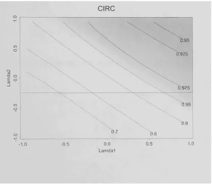
3.2.2 CIRC 42 3.2.3 DETACT-T2 43
3.3 Effect of Sample Size on ERMSE 45
3.3.1 Introduction 45 3.3.2 Methods 45 3.3.3 Results 46 3.4 Other Measures of Prediction Quality 46
3.5 Relationship between ERMSE and n 48
3.6 Discussion 49
4 A u g m e n t i n g C o m p u t i n g E x p e r i m e n t s 56
4.1 Introduction 56 4.2 Adding one run to a computer experiment 57
4.3 Adding more than one run to a computer experiment 59
4.4 Another Possible Approach 64
4.5 Discussion Go
5 A M o d e l for C o m p u t e r M o d e l s 68
5.1 Introduction 68 5.2 Simidating ASET-B 68
5.4 .A Computer Model Approach 80 5.5 Some Apphcations of the Results 83
5.6 Conclusions 83
6 Analysis of T i m e Traces 86
6.1 Introduction 86 6.2 Possible Methods 86
6.2.1 Separate Calculation for a Number of Time Points 88
6.2.2 Using Time as an Additional Input Factor 99
6.3 Conclusion 104
7 D i s c u s s i o n 105 7.1 Introduction 105 7.2 Limitations 107
7.2.1 Use of Latin Hypercube 107 7.2.2 Relationship between Sample Sizes and EMSE 107
7.2.3 Use of onh-Gaussian Product Correlation Structure . . . . 107
7.3 Future Work 107 7.3.1 AppHcation to other Designs 107
7.3.2 Application to other Computer Models 108
7.3.3 Prior Estimates of 9 and /; 108 7.3.4 Model Diagnostics for Time Trace Data 109
7.3.5 Multivariate Responses 109
Bibliography 110
List of Tables
2.1 Input Variables for ASET-B Fire Model 24 2.2 Scaled LHD points for ASET-B Input Variables. [Runs 1 to 25
of .Y = 50] and corresponding Egress Times. Coding scheme: scaled [—1,-1-1] input variables have been multiplied by 49. 25
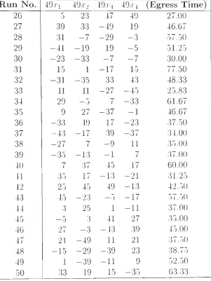
2.3 Scaled LHD points for ASET-B Input Variables. [Runs 26 to 50 of N — 50] and corresponding Egress Times. Coding scheme:
scaled [—1.-1-1] input variables ha\-e been multipUed by 49 20 2.4 Some suggested \-alues for ^s and ps from selected cases 28 2.5 Estiniatc^s of ^i d_i from 10 Random Starts with one Maximum
(12.12207) 29 2.6 Estimates of py p^ from 10 Random Starts with one Maximum
(12.12207) 29 2.7 Estimates of ^j 64 from 10 Random Starts with Different
Max-imum (MLE) 30 2.8 Estimates of p i , . . . ./^4 from 10 Random Starts with Different
Max-imum (MLE) 30 2.9 Estimates of Parameters for the ASET-B Computer Model 31
2.10 Functional ANOVA decomposition for the ASET-B experimental
data 39 3.1 Input Factors for D E T A C T - Q S Computer Model 42
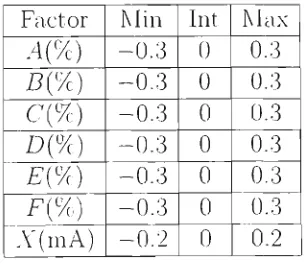
3.2 Minimum. Intermediate and Maximum le\-els of the controllable
factors for the C I R C Computer Model !•) 3.3 Manufacturing variations of the factors in the CIRC computer
3.4 Input Factors for D E T A C T - T 2 Computer Model 45 3.5 ERMSE for 3 LHDs for Sample Sizes of 10. 2 0 , . . . . 100 with the
ASET-B Computer Model 46 3.6 ERMSE for 3 LHDs for Sample Sizes of 10,20.... .100 with the
DETACT-QS Computer Model 47 3.7 ERMSE for 3 LHDs for Sample Sizes of 10,20,... .100 with the
CIRC Computer Model 48 3.8 ERMSE for 3 LHDs for Sample Sizes of 10,20,... .100 with the
DETACT-T2 Computer Model 49
3.9 Estimates of a, b and a 50 4.1 Coded design points of the Initial Design with Egress Times from
ASET-B 58 4.2 Results of Modelling ASET-B using the 20 run design gi^•en in
Table 4.1 59 4.3 Coded potential augmenting runs with Egress Times from ASET-B. 59
4.4 Ten Candidate Points following a Tweiit>' Points LHD for the ASET-B Fire Model; and MSE of Prediction for the 1st. 2ii(l
5th added points 61 5.1 Results for experiment on surrogate ASET-B model 69
5.2 Runs 1 32 of the Box-Behnken experiment on the ASET-B Fire
Model 72 5.3 Runs 33 64 of the Box-Behnken experiment on the ASET-B Fire
Model 73 5.4 Runs 65 96 of the Box-Behnken experiment on the ASET-B Fire
Model 74 5.5 Runs 97 130 of the Box-Behnken experiment on the ASET-B Fire
Model 75 5.6 Results for the Box-Behnken design on the ASET-B Computer Model 77
6.1 Scaled LHD points for ASET-B Input Variables, [Runs 1 to 25 of
A- = 50] 89
6.2 Scaled LHD points for ASET-B Input Wuiables. [Runs 26 to 50 of
A' = 50] 90 6.3 Scaled LHD points for ASET-B Input Variables. [Runs 1 to 25 of
A' = 50] and corresponding Egress Times from 0 to 30 seconds in
five second intervals 91 6.4 Scaled LHD points for ASET-B Input Variables, [Runs 26 to 50 of
A' = 50] and corresponding Egress Times from 0 to 30 seconds in
five second intervals 92 6.5 Scaled LHD points for ASET-B Input Variables, [Runs 1 to 25 of
A^ = 50] and corresponding Egress Times from 35 to 65 seconds in
five second intervals 93 6.6 Scaled LHD points for ASET-B Input Variables, [Runs 26 to 50 of
A' = 50] and corresponding Egress Times from 35 to 65 seconds in
five second intervals 94 6.7 Scaled LHD points for ASET-B Input Varial)les. [Runs 1 to 25 of
A' = 50] and corresponding Egress Times from 70 to 100 seconds
in five second intervals 95 6.8 Scaled LHD points for ASET-B Input Variables, [Runs 26 to 50 of
A' = 50] and corresponding Egress Times from 70 to 100 seconds
in five second intervals 96 6.9 Results of analysing Time Trace data using method 1 98
6.10 Predicted Response versus Actual response at five second time
inter^•als using method 2 102
List of Figures
2.1 Simple Illustration of ASET-B enclosure fire 20
2.2 Projection Properties of a LHD with 11 runs 23 2.3 Projection Properties of a LHD with 50 runs 27 2.4 Accuracy of Prediction for Egress Time 32 2.5 Main Effects plot for the ASET-B Computer Model 36
2.6 Interaction plot for the ASET-B Computer Model 37 2.7 Joint Effects for the ASET-B Computer Model 38
3.1 Diagram of Wheat stone Bridge 44 3.2 Scaled ERMSE \-ersus sample size for the four computer models. . 50
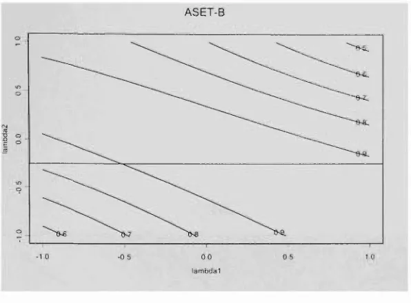
3.3 Rp versus sample size for the four computer models 51 3.4 Contour Plot of R^ v(>rsus Ai and A2 for ASET-B 52 3.5 Contour Plot of 7?2 versus Al and A2 for DETACT-QS 52
3.6 Contour Plot of 7?^ \-ersus Ai and A2 for CIRC 53 3.7 Contour Plot of 7?2 versus Al and A2 for DETACT-T2 54
3.8 Plots of Linear Relationship for Different Computer Models. . . . 54 4.1 Original 20 points from a LHD plus 10 labeled candidate points
from a 10 run LHD 60 4.2 Mean Square Error of Prediction adding one point at a time. . . . 62
4.3 Determinant of the variance-covariance matrix of predictions for all possible run combinations of five runs from the candidate set
of 10 runs 64 5.1 Comparison of Simulation Of ASET-B with actual results 70
5.2 Main effects plots for the model of computer models 79 5.3 Joint effect plot of n and p for the model of computer models. . . 80
5.4 Joint Effects of n and 6 for the model of computer models 81 5.5 Joint effect plot of 9 and p for a one-dimensional computer model. 82
5.6 Joint effect plot of 9i and p2 for the model of computer models. . 83 5.7 Joint effect plot of ^i and ^2 for the model of computer models. . 84 5.8 Joint effect plot of pi and p2 for the model of computer models. . 85 5.9 Comparison of results for ASET-B and predictions from the
quadratic-and marginal models 85 6.1 Generated Time Traces for the ASET-B Latin Hypercube
Experi-ment 88 6.2 Estimated 9s for Time in 5 second intervals 97
6.3 Estimated ps for Time in 5 second intervals 99 6.4 Predicted Response versus Actual response at 5 second time
inter-vals using; method 2 101
Chapter 1
Introduction
1.1 Computer Experiments
The advancement of high-speed computers has made experimentation \-ia com-puter modelling common in many areas of science and technolog>-. Comcom-puter modelling is having a significant impact on scientific research. \'irtually e\er>-a,rea. of science and technolog>' is affected. A computer model or simulator usu-ally involves complicated or high dimensional mathematical functions. Based on the mathematical formulation, the computer model or code produces outputs, if the reciuired \'alues of the input \'ariables are provided. Running the computer simulation can be expensive in different wa>'s. It can be labour intensive and/or time consuming. If the computer simulator is expensive to run, a natural straleg>' is to build a predictor from relativeh- few runs to act as a computationally less expensive surrogate (Welch et al. 1992) which can be used in a variety of waA's. for example during optimisation of the output.
In contrast. man>' complex processes that are conducted as physical (experi-mentation are too time consuming and expensi\'e (Sacks et al. 1989b). Moreover, for many s>-stems such as global weather modeling, en\-ironmental modelling and fire modelling, physical experimentation may simply be impossible. As a result. experimenters ha\'e increasing!}' moved to use mathematical models to simulate these complex systems. Enhancement of computer power has permitted b(jth
CHAPTER 1. INTRODUCTION 2
greater complexity and more extensi\e use of such models m scientific experi-mentation as well as in industrial processes. Computer simulation is imariabl)' cheaper than physical experimentation although these codes can be computation-ally demanding (Welch and Sacks, 1991).
This computer experiment approach has opened up a new avenue. "Design and Analysis of Computer Experiments" (DACE), which is somewhat different to the traditional methodology for the "Design of Experiments" (DoE). A signif-icant comparison between DACE and DoE concepts was presented b>' Booker ef
al. (1996). Booker (1996) compared DACE to DoE in three application areas:
electrical power system design, aeroelastic design and aerod\iiamic design. As Booker suggested "DoE and DACE . . . [are basically] the same approach
employ-ing different tools as appropriate''.
In general, computer models or codes consist of multivariate inputs. wJiich can be scalars or functions (Sacks et al. 1989b) and th(> resulting output from the same code may also be univariate and/or multivariate. In addition, the output can be a time dependent function and the enhanced abiUt\- to gather and analyse a number of summar\- responses \A-as highlighted by Sacks et al. (1989b). The input dimension differs according to the purpose and basis of the original computer model. Selecting a number of runs out of various input configurations results in Computer Expenments.
CHAPTER 1. INTRODUCTION .]
wer(> a mold filling process for manufacturing automobiles, chemical kinetic mod-els, a thermal energy storage model and the transport of pol>x>'clic aromatic hydrocarbon spills in streams using structured actiAit\- relationships model being of use in plant ecolog\-. In fact, the widespread use of computer models and ex-periments for simulating real phenomena generates examples in \irtuall\- all areas of science and engineering.
1.2 Role of Experimental Designs in DACE
Experimental design, as a statistical discipline, began with the pioneering work of R.A. Fisher in the 1920s. It is one of the most powerful tools of statistics and is widely used when designing experiments. Experimental designs have been used to mitigate the effect of random noise in experimental outcomes. Howe\'er, the ke>' ideas of randomisation, replication, and blocking are not useful for computer experiments.
In contrast, the Design of Computer Experiments is a new a\'enue in the Design of Experiments since there are no random errors. Also, replication is not uecc^ssary since one always obtains the same response at the sam(> iiii)ut settings (Booker 1996). The role of statistical experimental design in Computer experiments was reviewed by Sacks et al (1989b), stating that . . . . " the selection
of inputs at which to run a computer code is still an ciperiniental design problem ".
1.3 Differences between Computer Experiments
and Other Experimental Design
AUhough Factorial and Fractional Factorial designs are most commonly used for physical experiments, in computer experiments perhaps the most common designs are Latin Hypcncube Designs (LHD). These were the first type of designs to be explicitly- considered as experimental designs for deterministic computer codes.
CHAPTER 1. INTRODUCTION 4
code with the same inputs will be identical. Since these models have no ran-dom or measurement errors, computer experiments are different from physical experiments calling for distinct techniques for design. These deterministic com-puter experiments differ substantially from the niajorit}' of ph>-sical experiments traditionally performed by scientists. Such experiments usually haA-e substantial random error due to variabihty in the experimental units (Sacks et al. 1989b).
The remarkable methodology of statistical design of experiments was intro-duced in the 1920's and popularised among scientists following the publication of Fisher (1935). The associated analysis of variance is a systematic wa>- of sep-arating important treatment effects from the background noise (as well as from each other). Fisher's methods of blocking, replication and randomization in these experiments reduced the effect of random error, provided valid estimates of un-certainty and preserved the simplicit>' of the models. The deterministic computer codes considered in this thesis differ from codes in the simulation literature (Sac ks
et al 1989b), which incorporate substantial random error through random
num-ber generators. The random (as opposed to deterministic) simulation, i.e., com-puter models that use pseudorandom numbers (as in man>' telecommunications and logistic applications) described by Law and Kelton (2000) is a significant contribution for simulation experiments. It has been natural, therefore, to design and anah'se such stochastic simulation experiments using standard techniques for pliA'sical experiments. Howevcn'. it is doubtful whether these methods are ap-propriate for computer experiments considered here since the prediction wiU not then inatcli the observed deterministic respomse. For this reason other methods of design and anah'ses haA-e been de\-eloi)ed 1J\- a number of authors.
The design problem is the choice of inputs for efficient analysis of the data. A c'omputer experimental design consists of a set of sample points to be evaluated through the computer code or model. The observations from this design are tlieii used to develop a computationally cheaper surrogate model to the code. This n(>w model is used to estimate the code inexpensively and efficienth-. to iii\-es-tigate the behavior of the function, or to optimise some aspect of the function.
CHAPTER 1. INTRODUCTION 5
unkrioIvn function and providing an approximating model that can be nif.rjMiisieelij evaluated" (Koehler and Owen, 1996).
1.4 Designs for Computer Experiments
McKay et al. (1979), were the first to exphcitly consider experimental de-sign for deterministic computer codes. With the input variable giA-en 1)\- X =
(X^,... ,X^) where X^ is a standardised input between 0 and 1. and the output
produced by the computer code given by y = /^(X), they compared 3 methods of selecting the input variables:
1. Random Sampling
2. Stratified Sampling
3. Latin Hypercube Sampling - an extension of stratified sampling which en-sures that each of the input \-ariables has all portions of its range repre-sented. A uniform Latin II\-percube sample of size n has
A7 = ^ ^ ^ ^ - ^ . l < ^ < n . l < . 7 < f /
n
n.
where 7rj(l) 'T"J('0 ^^6 random permutations of the integers 1,.
Uj '^U[0,1] and the d permutations and nd uniform variates are mutuall\'
independent (Owen. 1992a). Many authors use the simpler Lattice samijle. following Patterson (1954), where
A7 = !l(!l_zi. l < ^ < n . l < ; < d .
n
A slightly altered definition has been used in this thesis.
CHAPTER 1. INTRODUCTION 6
allowed for different assumptions on the input variable to be studied without ad-ditional computer runs. Iman and Conover (1982) showed how Latin H>-percube Samples could be modified to incorporate the correlations that ma>- exist among the input variables. The method was used on a model for the studA- of Geological Disposal of Radioactive Waste. Stein (1987) ga\-e the asymptotic \'ariance of the Latin Hypercube based estimation and showed that the estimate of the expected value of a function based on a Latin H>-percube sample is asA'mptotically normal and that the improvement over simple random sampling depends on the degree of additivity of the function of the input variables. He also provided a better method than Iman and Conover (1982), of producing Latin Hypercube sampling when the input variables are dependent.
Other experimental designs based on different optimality criteria w-ere stud-ied by Koehler (1990) who considered Entropy. Mean Square Error. Minimax. Maximin and Star-discrepanc\- based designs. In addition, three examples were studied: one a chemical kinetics prolDlein involving 11 differential equations. The second example investigated was a large linear s>-stem of differential ec(uations involving methane combustion with s(>\-en rate constants regarded as inputs. To reduce the computer time, the design is restricted to a central composite design t.\-i:)e (Box and Draper, 1987) but witli unknown shrinkage factors for the cube points and the star points of the design.
A number of computational methods for augmenting the design were described which would be classified as single stage methods, sequential methods without adaptation to the data, and seciuential methods with adaptation. The problem of how to design an augmenting experiment is an important one. It is clear, hoAvever. tliat much more work needs to be done to make these methods easier to use and this is something this research stud>- aims to accomplish.
CHAPTER 1. INTRODUCTION 7
sample is giA-en b>'
.X; = i M i l i l . 0 < , < 1 , 0 < ; < - 1
Q
where the TTJ are independent permutations of 0 ,q — I and .4^ is the Aalue of the i'^ row and j ^ ' ' column of an orthogonal arra>-. Similarl>-. Lattice samples can be generalised b>' taking
Owen (1992b) suggests that the arrays OA{q'^. k, q, 2) are a good choice for com-puter experiments since the n = q^ points plot as a g x g grid on each bivariate margin. He also presents OA of strength 2 of the form OA {q^.q + L g , 2 ) for
q = 2 , 3 . 4 , 5 , 7 , 8 , 9 , 1 1 . 1 3 , 1 6 , 1 7 , 1 9 , 2 5 , 2 7 . and 32 and OA {2q^,2q ^-l.q,2) for q = 2 , 3 , 4 , 5 , 7 , 8 , 9 , 1 1 , 1 3 , 1 6 although the latter designs include the same
pro-jections in three columns that include repeat runs, an undesirable feature for a computer experiment. In a later paper, (Owen 1994b), it is conjectured that sub-arrays of the form OA {2q^.2q.q. 2) do not have this defect.
Owen (1992a) also suggests wa>-s to augment a computer experiment. If an experiment based on an OA {q. d. q. 1) has been run then it can be used as an angnienting set for those runs that would complete an OA {2q. d. q. 1). If we want to increase the number of \-arial)les then OA {q^. d. q. 2) x OA (g^, (P, cf. 1) could be used.
Independent to the work of Owcni. Tang (1993) also generalised Latin lly-j)ercul)es b>- developing Orthogonal ArraA- based Latin Hypercube Designs. OA based Latin Hypercubes offers a substantial improvement over Latin H>-per(ube sampling and are proposed to be a more appropriate design for Computer Exper-iments.
CHAPTER 1. INTRODUCTION 8
an experimental design to be used in Computer Experiments for DACE would gi\-(^ more confidence because of its good space-filling properties and infiltration of the design space. He gaA-e examples A\-here he had used OA-based Latin H\--percube samples which are derived from OAs, for an areoelastic simulation of the performance of a helicopter rotor.
1.5 Analysis of Computer Experiments
In a computer experiment, observations are made on a response function y b\-running a (typically complex) computer model at \^arious choices of input factors X. For example, in the chemical kinetics of methane combustion, x can be a set of rate constants in a system of differential equations and y can he a concentration of a chemical species some time after combustion. Soh-ing the differential equations numerically for specified x >-ields a value for y. Because running the equations soh'er is expensive, the aim is to estimate the relationship between x and y from a moderate number of runs so that y can be predicted at untried inputs.
Extracting observations from this design can be used to build up a computa-tionalh- inexpensive surrogate model to the selected simulator or coni])uter code. This surrogate model is used to approximate the computer simulator or model cheaply and efficientl>-. to iin'estigatt^ the behaviour of the function and/or to optimise some aspect of the function.
A major contribution to the area was made by Sacls;s et al. (1989a). The response \\-as modeled as:
Response = Linear Model -I- Departure
k
yW = 5].i,/,(x) + z(x).
CHAPTER 1. INTRODUCTION 9
to two r/-dimensional inputs t = (ti /,/) and u = {ui....)i,i) is given by.
d
Coy{z{t).z{u)) = alY[Rj{t^.Uj) (1.1)
i = i
where
Rjilj.uj) = exp{-9{t,-u,)'). (1.2)
Here ^ > 0 defines the correlation structures of z and cx^ is a scale factor. T h e authors discussed the importance of the parameter 6. When 9 is large there is small correlation between observations and therefore prediction is harder. On the other hand when 9 is small there is large correlation between observations and prediction is much easier. Selection of the correlation function plaA-s a critical role in the prediction process. Koehler (1990) discussed different correlation families and their suitabilit.\- to the prediction process and the effects of 9 on prediction.
Given the model above the authors deriA-ecl the Best Linear Predictor and the mean square error of prediction. To come up with a design the>- tr>- to minimize the integrated mean square error (EMSE) of prediction. The IMSE is given by
JeiS.Y) = [llaD j Ee{Y{yi)-Y{^))hlx
where V'(x) is the Best Linear Predictor, (5) is the design, the design-prediction strategA' is {S. Y) and the integration is OA^er the region of interest.
Since there usualh' is no AvaA- of guessing the A^alue of 9 prior to the experiment the strategy adopted bA- the authors is to choose a A^alue of 9. sav 9\. that gi\-es a design-prediction strategA- that performs well for a A\-ide range of true (but unknown) 9T- A number of different values of 9\ are chosen and for each the optimal design SQ^ and Best Linear Predictor Yg^ are found. Then for various A'alu(\s of 9T the IMSE Jej.{Se^^.Ye^) is calculated. This quantitA' is a measure of the ])(nforiiiance of the strategy [SQ^, YQ /) when 9^ is true.
A measure of relative efficiencA- is
CHAPTER 1. INTRODUCTION 10
A robust strategy is to choose 9A SO that these relatiA-e efficiencies are as ( onstaiit as pos,sil)le.
The paper In- Sacks et al (1989b) Avas also very important. The objectiA-es of a Computer Experiment are set out as:
1. Predicting the response at untried inputs
2. Optimizing a function of the response
3. Validation and Verification (Matching the computer code to physical data). Kleijnen (2000) highlighted the importance of the A^alidation and verifica-tion in the simulaverifica-tion experiments. The author has claimed the A^alidaverifica-tion and verification has many facets, including philosophical and mathematical-statistical problems. In particular, the author stressed "In praetice, even ciuite simple simulations are not validated through correct statistical tech-nic|ues" [see Sargent et al, (2000) for more details]
Sacks et al (1989b) concentrated on the first objectiA-e. The basic statistical ciuestions Avere:
• The design problem:
At which input "sites" S = ( s i , . . . , .s„) should the data y{sy)... y{sn) be calculated ?
• The anal\-sis problem:
HoAv should the data be used to meet the objectiA-e '.''
They c laimed that statistics had a role in Computer Experiments since selection of inputs at \\-hich to run a computer code is an Ex]>erimental Design problem and the quantification of the uncertaintA- associated with prediction from fitted models is a statistical problem.
TAVC) rationales for modeling the deterministic departure as a realisation of a stochastic process Avere adA-anced:
CHAPTER 1. INTRODUCTION 11
Kriging
Kriging is named after the South-African mining engineer D.G. Krige. It is an interpolation method that predicts unknown A'alues of random function or random process (Cressie, 1993). More precisely, a Kriging prediction is a weighted linear combination of all output values already obserA^ed. These weights depend on the distances betAveen the location to be predicted and the locations already observed. Kriging assumes that the closer the
in-put data are, the more positively correlated the prediction errors are. This
assumption is modeled through the correlogram or the related variogram. Kriging is popular in deterministic simulation. Compared AA-ith linear re-gression analysis, Kriging has an important adA-antage in deterministic sim-ulation: Kriging is an exact interpolator: that is. predicted A-alues at ob-served input values are exactlA- eciual to the obserA^ed (simulated) output values [Kleijnen and A^an Beers (2003)].
2. y(.) may be regarded as a Bayesian prior on the true response function, Avith the 'Ts either specified a priori or given.
The Best Linear Predictor Estimate^ (Welch et al. 1992) Avas USCHI - this is related to the concept of Krigmg in the Geostatistical literature (Cr(\ssie, 1986). Alternativeh- the posterior mean could be used from a Bayesian A-ieAV]3oint.
The correlation function used f)>- Sacks al al. (1989b) includes a different 9 for each input,
d
7?(w.x) = llexp {-9,\w, - x,\n (1.3) j = i
and the authors also foreshadoAA- the use of a different pj, for each input. If the model is
y(x) = ,.3 + z(x) (1.4)
then obtaining the maximum likefihood estimators of 9i,....9d, p. p and a^ reduces to numericallA- optimizing
I
CHAPTER 1. INTRODUCTION 12
where RD is the matrix of correlation for the design points.
3 = ( l ^ R B ^ l ) - ^ l ^ R - i ( y ) (1.6)
and
a 2
1
iy-13fR^'(y-lJ}. (1.7) n
The quantity to be optimised is a function of only the correlation parameters and the data.
Given the correlation parameters, [In practice, these parameters are not giA^en but are estimated. For an update see Kleijnen and Van Beers (2003)] the next step is to build the best linear unbiased predictor (BLUP), y(x). of y(x). The BLUP for an untried x is
y(x) = J + r^i^H^iy-lJ) (1.8)
A\4iere
r(x) = [i?(xi,x) R{^n.^)V (1-9)
is the A-ector of correlations Ijetween the ;s at the design points [ x i . . . . ,x„] and at an untried input x. Since /?(x, x) = 1, the predictor Avill interpolate the data points, as it should if the data are Avithout random error (Welch, et al. 1992).
The prediction error for y(x) can be presented on the basis of the model considered in this thesis as
-1 MSE[y(x)] = a 2
1 - 1 r ^ ( x T.IO)
A numbcn- of design criteria were considered \A-ith the objectiA'c of choosing a design that predicts the response AA-CII at untried inputs in the experimental region. In the Integrated Mean Square criterion the objective is to minimize
/ MSE[y(x)]f/x
JxER
CHAPTER 1. INTRODUCTION 13
to minimise the maximum MSE although this is much more computationally de-manding. A third criterion is the maximization of expected posterior entropy (amount of information aA-ailable to the giA'en experimental region). The asymp-totic connection betAA^een the maximization of expected posterior eiitrop\- criteria (as est,al)lished by Johnson et al, 1990) is the need to in.sure that the design will be effective even if the response A-ariable is sensitiA-e to only a fcAv design variables. The goal of this is to find designs which offer a compromise between the entroi)y maximin criterion, and projectiA-e properties in each dimension of the response variable (Morris and MitcheU, 1995). An approach In- Ye et al,
(2000) on such "compromise between computing effort and design optimalitA-"" is a significant improvement on constructing designs for computer experiment. The authors claimed that the proposed class of designs [Symmetric Latin h}'percube Design (SLHDs)] has some advantages over the regular LHDs AA-ith respect to criteria such as entropA' and minimum intersite distance. The authors also claimed that SLHDs are a good subset of LHDs witli respect to both entropy and maximin distance criteria (for a comprehensi\-e discussion see Ye et al, 2000).
A number of interesting points A\-er(^ mack> in the discussion of the paper bv Sacks et al. (1989b). Some of the discussants raised the possibility of using factorial or fractional factorial design as cheap and simple designs that are nearh-optimal in maiiA- cases. In their repl,\- the authors made the claim that suitablA-scaled half fractions are apparentl>- optimal or close to optimal for the IMSE criterion for the model Avith onl>- a constant term for the regressicm and p = 2. A number of the discussants also examined the correlation function and stochastic-process models and caUed for additional work in this area.
A BaA-esian approach was adopted by Currin et al (1991). They considered product of linear correlation functions
R^d) = I - j\d\. 4 < ^ < o c
and
R{d) = l - | | c i | , | r / | < ^
CHAPTER 1. INTRODUCTION 14
and also product cubic correlation functions
Rid) = l - 6 ( f ) 2 + 6(M)3. \d\<l,
= 2 ( l - ^ ) ^ f<ici|<^,
= 0, \d\ > 9 where ^ > 0 and
k
R{d) = l[R{d,).
The prediction functions are respectiveh- hnear or cubic splines in e\-erA- dimension (Venables and Ripley, 1995, page 250). The design used Avas that Avhich minimises the posterior entropy (SheAvry and Wynn, 1987).
The authors gave a computational algorithm for finding entropA--optimal de-sign on multidimensional grids. The authors found. hoAvcA-er, that for some of the examples considered and for some correlation parameters the 95 pcncent poste-rior probabilitA' intervals do not giA-e aclec[uate com^ergence of the true A-alues at selected test sites.
Welch et al (1992) extended prcAdous results to consider larger numbers of predictors in the case where there are OUIA' a feAv actiA-c- factors. The correlation function considered was
/2(w,x) == lleM-9,\ir,-.r,n.
j = i
Although full maximum likelihood could be used it Avould be numericallA-costlA-. Instead each of the 9j is set equal to each other, similarly for the pj. The first stage is to maximize the likelihood based on the common A-alues of 9 and p. Then a stepAvise procedure is used so that a 9j and Pj is introduced for that A-ariable for Avhich such a step most increases the likelihood. The procedure continues until giA'ing am- of the remaining factors their OAvn values of 9j and j)j does not make a large difference relatiA-e to the previous stage.
CHAPTER 1. INTRODUCTION 15
Good starting Aalues are also obviously an important part of the MLE calculation. There is \-ery little hterature on how to get good starting values. One exception is Owen (1994a) AVIIO gaA^e a method for estimating 9i... . ,9^ AA^hen p = I Avhich could be used as starting A-alues in the maximum likelihood estimation.
A number of examples were presented In- Welch et al. (1992). For one example involving only two A^ariables a 50 run Latin HA-percube Avas shoAvn to giA-e good results. However, a 30 run and 40 run design does not identify a reasonable model. No guidelines for the appropriate sample size are giA'en. In the second example a 50 run Latin Hypercube Avas successful in identifying fiA-e significant factors. The number of runs required for a computer experiment remains a kcA' open question and is one that this research aims to tackle.
1.6 Thesis Outline
The thesis consists of seven chapters. The first chapter is a general introduction and Literature RcA-iew of the area of computer experiments.
In the second chapter a simple computer model Avill bc^ introduced for the purpose of describing exacth- Avhat a computer model is. hoAv it can be USCHI and Avhat problems Avill be addressed in the thesis. The approach of modeling the deterministic model as a stochastic process \\-ill be described. Focus Avill be on important practical issues that haA^e not receiA-ecl much attention in the literature such as starting A-alues, parameterization and generating plots for interprc-tation. The third chapter Avill focus on the effect of sample size (the number of com-puter experiments) on the precision of the predictions based on the fitted stochas-tic model, parstochas-ticularlA- in the case Avhen a Latin HA-percube design is used.
The fourth chapter Avill examine hoAv to add extra runs to a computer experi-ment in order to improve the precision of t he predictions. TAVO approaches Avill be examined, one adding one point at a time Avhile the other adds groups of points at a time.
CHAPTER 1. INTRODUCTION 16
experiments is used to stud\' computer experiments themseh-es. This is likelA' to give results that are more general than the specific results deA'eloped in Chapters 3 and 4.
Many computer models giA-e the response as a function of time. HoAveAer most of the literature on computer experiments focused on each run of the code giAdng one response value. In Chapter 6 methods will be deA-eloped to efficientlA- analyse the multivariate data generated by a computer code.
C h a p t e r 2
Analysis of a Simple C o m p u t e r
Model
2.1 Introduction
Since this thesis focuses on a number of ])ractical issues relating to the design and analA'sis of computer experiments, it is of xalue here to descrilx* one model in detail. This material Avill be used in later chapters. The particular (^xample selected is A\-ailable Safe Egress Time (ASET-B), a computer model predicting the nature of a fire in a single room, presented l)y Walton (1985).
A Latin Hyi)ercube Design (LHD) is used to choose input factors for the ASET-B program. Based on this LHD, responses (y) from the model are gener-ated to form a computer experiment. The responses are modeled as thc> realisa-tion of a stochastic process, folloAving the AA'ork of Sacks et al. (1989a). Maximum Likelihood Estimates (MLE) of the parameters are generated and these estimates used to make predictions at untried inputs. The prediction can be made using the Best Linear Unbiased Predictor (BLUP), a methodology introduced by Hen-derson (1975b) and Goldberger (1962). A graphical interpretation of the results is presented.
CHAPTER 2. ANALYSIS OF A SIMPLE COMPUTER MODEL 18
2.2 Deterministic Fire Models
A stochastic process involves chance or uncertaintA-. In a deterministic \A'orld everything is assumed certain. Deterministic fire models attempt to represent mathematically the processes occurring in a compartment fire based on the laAvs of physics and chemistry. These models are also referred to as room fire models, computer fire models, or mathematical fire models. Ideally, tliCA- are such that discrete changes in any physical parameter can be evaluated in terms of the effect on fire hazard. While no such ideal exists in practice, a number of computer models are available that provide a reasonable amount of selected fire effects (Cooper and Forney, 1990).
Computer models have been used for some time in the design and analysis of fire protection hardware. The use of computer models, commonly knoAvn as design programs, has become the industry's standard method for designing \A-ater supply and automated sprinkler SA-stems. These programs perform a large number of tedious and lengtln- calculations and provide the user Avith accurate, cost-optimised designs in a fraction of the time that AA-ould be rec|uired for manual procedures.
In addition to the design of fire protection hardw-are, computer models nuu-also be used to help CA-aluate the effects of fire on both people and propertA'. fhe models can provide a fast and more accurate estimate of the impact of a fire and help establish the measures needed to prcA-ent or control it. Wliile manual calculation methods provide good estimates of specific fire effects (eg., prediction of time to flash OA^er), they are not well suited for comprehensive aiial\-sis iuA-oh'-ing the time-dependent interactions of multiple physical and chemical processes prc\sent in developing fires.
2.2.1 The ASET-B Fire Model
CHAPTER 2. ANALYSIS OF A SIMPLE COMPUTER MODEL 19
Avritten in FORTRAN by Cooper (1980). Later, Walton (1985) implemented the model in Basic as ASET-B incorporating simpler numerical techniques to sohe the differential equations involved.
ASET-B is a personal computer program for predicting the fire emironment in a single room enclosure Avith all doors, Avindows and A-ents closed except for a small leak at floor level. This leak preAents the pressure from increasing in the room. A fire starts at some point below the ceihng and releases energy and the products of combustion. The rate at Avhich these are released is likely to change Avith time. The hot products of combustion form a plume Avhich, due to bu(j>-ancy, rises. As it does so, it draAvs in to the room cool air Avhich decreases the plume's temperature and increases its A'olume fioAv rate. Wlien the plume reaches the ceiling it spreads out and forms a hot gas laA-er \A-hich descends \A-ith time as the plume's gases continue to floAv into it. There is a relatiA-(4A- sharp interface betAveen the hot upper laA-er and the air in the loAver part of the room which, in the ASET-B model, is considered to be at ambient tempcTature. The only interchange betAveen the air in the loAver part of the room and the hot upper layer is through the plume.
ASET-B SOIA'CS scA-eral differential equations using a simpler numerical tech-nique than in the original ASET program. ASET-B requires as inputs the height and area of the room, the elevation of the fire aboA-e the floor, a heat loss factor (the fraction of the heat released b}- the fire that is lost to the bounding surfaces of the enclosure) and a fire specified in terms of heat release rate w-hich depends on the nature of the combustion material. For this study I ha\e used the ratc> of release for a 'semi-uniA-ersal fire", corresponding to a "fuel package consisting of a polyurethane mattress with sheets, fuels similar to AA^ood cribs and polyurethane on pallets, and commodities in paper cartons stacked on paUets"' (Birk 1991, page 86). The program predicts the thickness and the temperature of the hot smoke hiA-er as a function of time. A simple illustration of fire-in-enclosure floAv clA-iiam-ics for an "uiiA-ented'" enclosure and the basic fire phenomena are presented in Figure 2.1.
CHAPTER 2. ANALYSIS OF A SIMPLE COMPUTER MODEL 20
la\-c>r to be at 5 ft (head height). This manipulation was carried out in order to make the output uniA-ariate. The analysis of profiles OA'er time is presented in chapter 6.
F — Height of base of fire H — Height of room
nie — IMass AOAA- rate leaA-ing crack like \-eiit nip — Plume mass floAv rate
Qc — Convective energA" release rate Qr — RadiatiA-e energA- release rate Q(t) — Heat release rate at time (t)
X — Height of interface aboA^e floor Zi — Interface height aboA^e fuel surface.
CHAPTER 2. ANALYSIS OF A SIMPLE COMPUTER MODEL 21
2.3 Experimental Design
2.3.1 Latin Hypercube Designs
There are many experimental designs available for computer experiments. These designs include the folloAving: Random Latin Hypercubes [McKa.A-. et al 1979], Random Orthogonal Arrays (Owen, 1992b), IMSE Optimal Latin Ilvpercubes
(Park, 1994) and (Sacks, et al 1989b), Maximin Latin Hypercubes [MmLh] (Morris and MitcheU, 1995) and (Johnson, et al 1990), OrthogonaUArrav based Latin Hypercubes [Tang (1993) and Owen, (1992b)], Uniform Designs (Fang and Wang, 1994), Orthogonal Latin Hypercubes (Ye 1998), Hammersley Sequence Designs (Kalagnanam and Diwekar, 1997), Symmetric Latin Hypercubes (Ye et
al 2000) and Minimum Bias Latin Hypercube Design [MBLHD] (Palmer and
CHAPTER 2. ANALYSIS OF A SIMPLE COMPUTER MODEL 22
the benefits of elaboratc> and efficient importance sampfing strategies. Therefore. Latin liA-percube sampling has the qualifications to become a widelA- emploA-ed tool in rehabihty analysis." (Olsson et al. 2003).
A LHD gives an evenlA- distributed projection into each of the input factors. With this choice in a sample of size W the / ' * obserA-ation for the /"" \-ariable is given as
^j / M a x , - M i n A / M i n , + MaxA . ^ , . ^ ^.
^'- = [ 2 )''-'[ 2 ) ' = l---^/^^ = l -^
where Max, is the Maximum of X,. Min, is the Minimum of X,-, , _ 2 ^ , ( z ) - W - l
r: N-V
and 7Tj{i) is the j " * obseiA-ation of a random permutation of the integers 1 , . . . . A'. 7r(j) = (7rj(l),. . . , 7rj{N)) and the d random permutations 7 r ( l ) , . . . . 7r(d) corre-sponding to the d input factors are mutually independent. Note that —1 to 1 has been chosen as the range for the coded in])uf factors, .r,, although some authors (Sacks et al. 1989b) prefer a range of 0 to 1.
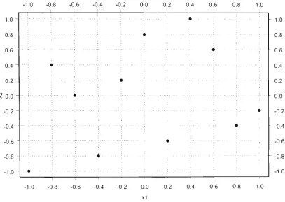
A simple LHD (W = 11), for a two dimensional (.r| and X2) case is illustrated in Figure 2.2 and shoAvs that each of those components is represented in a full\-stratified manner. Note tiiat each component is sampled uniformly on the inter\-al
[-1^1]-2.3.2 A p p l i c a t i o n t o A S E T - B C o m p u t e r E x p e r i m e n t
The first stages of a computer experiment involve selecting the input variables and the ranges OA^er Avhich they Avill be explored. For the ASET-B model the inputs were taken to be the Heat Loss Fraction, the Fire Height, the Room Ceihng Height and the Room Floor Area giAing a four dimensional configuration. The ranges of the \^ariables are giA^en in Table 2.1.
CHAPTER 2. ANALYSIS OF A SIMPLE COMPUTER MODEL 23
1.0
0.8
0.6
0.4
0.2
! 0.0
-0.2
-0.4
-0.6
-0.8
-1.0
-1.0 -0.8 -0.6 -0.4 -0.2 0.0 0.2 0.4 0.6 0.8 1.0
- 1 I ! ! ! I I I I i L _
n i i 1 1 \ 1—
-1.0 -0.8 -0.6 -0.4 -0.2 0.0 0.2
xi
0.4 0.6 0.8
- 1.0
- 0.8
- 0.6
0.4
0.2
0.0
' -0.2
- -0.4
- -0.6
~ -0.8
-1.0
1.0
Figure 2.2: Projection Properties of a LHD with 11 runs.
The number of runs required remains an open ciuestion for computer exper-iments. Welch et al' (1996) suggest, as a guidefine. that the- number of runs in a computer experiment should be chosen to be 10 timers the number of actiAc inputs, Avhich would lead to A' = 40 runs for this example if all four factors turn out to be actiA-e. To be conservatiA-e Y = 50 runs Avas used. More on sample size considerations will be discussed in Chapter 3.
CHAPTER 2. ANALYSIS OF A SIMPLE COMPUTER MODEL 24
Variable
X,
X2
X, X,
Variable name Heat Loss Fraction Fire Height (ft)
Room Ceiling Height (ft) Room Floor Area (sq. ft)
Minimum 0.6 1.0 8.0 81.0
Maximum 0.9 3.0 12.0 256.0
Table 2.1: Input Variables for ASET-B Fire Model
2.4 M o d e l l i n g
2.4.1 S u m m a r y of t h e A p p r o a c h used by Sacks et aL
Modelling for the ASET-B responses were carried out as a realization of a stochas-tic process, following the methodology dcA^eloped by Sacks et al. (1989b).
The response y(x) is assumed to folloAv Equation 1.4 Avhere the sA-stematic component z(x) is modefled as a realisation of a Gaussian stochastic process in Avhich the covariance function of -:(x) relates to the smoothness of the r(\s])onse. The covariance of the responses to two d-dimensional inputs t = [ti.... .t^) and u = ((/i,. . . ,Ud) is giA-en by Ecjuation 1.1 and Eciuation 1.2
2.4.2 M a x i m u m Likehhood E s t i m a t i o n
Sacks et al. (1989b) shoAv that obtaining the maximum hkefihood estimators of
9i 94.P1, • • • -P^- '^ and cr^ reduces to numerically optimising Eciuation 1.5,
Avith j] giA-en Ijy Equation 1.6 and (7^ given by Equation 1.7. Note that the ciuantity to be optimised is a function of only the correlation parameters, {9j and
Pj) and the data.
Starting Values
After assigning the inputs to LHD for different sizes of A', the next step is to choose starting A-alues for the Maximum Likehhood Estimation. Calculation of the maximum likelihood estimates depends on good starting values. To studA- a suitable distribution for starting values, some A-alues listed in the literature for
CHAPTER 2. ANALYSIS OF A SIMPLE COMPUTER MODEL 25
Run No.
1 2 3 4 5 6 7 8 9 10 11 12 13 14 15 16 17 18 19 20 21 22 23 24 25 49xi -37 23 37 -17 -47 49 11 17 -19 -25 -13 47 -45 -11 -49 -21 13 -29 19 -9 43 -1 -3 — 7 -39 49.r2 -11 -31 5 11 -25 39 -9 -1 31 43 -21 21 -47 15 29 9 47 -37 -45 -27 13 -15 -41 35 -43 49x3 -31 -19 -41 25 -3 27 43 29 37 -45 -35 21 -15 -33 31 13 -21 -23 -25 35 23 -47 3 9 5 49.X4 -27 -19 -49 25 35 31 45 5 -41 47 -25 33 41 -47 -9 13 -39 -29 -43 1 3 29 -15 -31 37(Egress T i m e ) 26.00 58.33 36.25 48.75 40.00 25.83 55.00 61.67 55.00 34.00 43.00 63.33 73.33 43.75 33.00 61.67 35.00 48.75 61.67 56.67 48.33 33.00 58.75 47.50 56.25
CHAPTER 2. ANALYSIS OF A SIMPLE COMPUTER MODEL 26
Run No.
26 27 28 29 30 31 32 33 34 35 36 37 38 39 40 41 42 43 44 45 46 47 48 49 50 49.ri 5 39 31 -41 -23 15 -31 41 29 9 -33 -43 -27 -35 7 35 25 45 3 -5 27 21 -15 1 33 49:r, 23 33 —7 -19 -33 1 -35 41 —5 27 49 -17 7 -13 37 17 45 -23 25 3 -3 -49 -29 -39 19 49x3 47 -49 -29 19 -7 -17 33 -27 7 -37 17 39 -9 -1 45 -13 49 —5 1 41 -43 11 -39 -11 15 49.r4 49 19 -3 -5 -7 15 43 -45 -33 -1 -23 -37 11 7 17 -21 -13 -17 -11 27 39 21 23 9 -35(Egress T i m e ) 27.00 46.67 57.50 51.25 30.00 77.50 48.33 25.83 61.67 46.67 37.50 34.00 35.00 37.00 60.00 31.25 42.50 57.50 37.00 35.00 45.00 37.50 38.75 52.50 63.33
CHAPTER 2. ANALYSIS OF A SIMPLE COMPUTER MODEL 27
X1
• . • • . _
•^.0 -0,5 0.0 0,5 1,0
• , * ' ,
X2
• . '
• . * • • . • .
1,0 -0 5 0,0 0 5 1,0
• ' • •
' . , • •
'. • \ •
. • . • • • . '
. " • •
• • .
X3
• ' . •
. • .
X4
-1,0 -0,5 0,0 0,5 1,0 -1,0 -0,5 0,0 0,5 1,0
Figru'e 2.3: Projection Properties of a LHD with 50 runs.
According to the indicated magnitudes of ^'s and p's: the ^s lie between 0 and 2 and the ps will also be bet\\-een 0 and 2.
Based on this evidence, the method adopted Avas to generate^ 10 random sets of starting A-alues and for each set to calculate the maximum likelihood estimates. The random starts for the parameters Pj, j = 1,... ,d, were generated from a uniform distribution on [0,2], AA-hile the random starts for the 9j. j = 1, d. w-ere generated from an exponential distribution Avith mean 1. Of course other distributions could be used.
Calculating the maximum likelihood estimates is a constrained optimisation problem since 0 < Pj < 2, j = 1.. .d and 0 < 9j j = 1.. .d.
CHAPTER 2. ANALYSIS OF A SIMPLE COMPUTER MODEL 28
Citation
Sacks et al (1989b) Koehler (1990)
Welch et al (1992)
Booker (1998) Chang et al (1999)
Case 1 2 3 4 5 6 7
"min 0.00 0.00 0.00 0.00 0.00 -0.4 0.00
"max 1.970 1.800 1.850 0.036 0.970 0.4 2.00
Pmin Pmn.T 1.61 2.00 1.00 2.00 2.00 2.00 1.70 2.00 1.61 2.00 0.00 0.25 0.00 2.00
Table 2.4: Some suggested values for ^s and ps from selected cases.
rpj and qj, j = 1,... ,d, where
© 7
Qj
By using the likelihood based on the Oj and cjj, com-ergence Avas achieved much quicker than using the likefihood based on the 9j and j)j. Once the com-erged values of (j)j and qj are obtained the estimated \-alues of 9j and Pj are giA-en
b\-o -,
2
^^ (expgj)2'
As a preliminarA- experiment tAvo sets of ten random starting values for the ASET-B model AV(^re generated. The results for the first set of starting \-alues are given in Table 2.5 and Table 2.6. AU ten starting A-alues give the same maximum likelihood estimates (-loghkelihood = 12.12207). The resufis for the second set of ten starting values are giA-en in Table 2.7 and Table 2.8. In contrast to th(^ first set, the second set gave four different likelihood modes. The mode that occurs most often appears to be the maximum likelihood and giA-es the same loghkelihood as in the first case.
2.4.3 Apphcation to ASET-B Computer Experiment
CHAPTER 2. ANALYSIS OF A SIMPLE COMPUTER MODEL 29
Random Start 1
2 3 4 5 6 7 8 9 10
9i 02 9-, 6*4
0.0000000 0.1512159 0.0008050 0.2441341 0.0000000 0.1511380 0.0008048 0.2444890 0.0000000 0.1512156 0.0008011 0.2445132 0.0000000 0.1510373 0.0008084 0.2484577 0.0000000 0.1510374 0.0008084 0.2484576 0.0000000 0.1512159 0.0007999 0.2451331 0.0000000 0.1510375 0.0008084 0.2484577 0.0000000 0.1510374 0.0008084 0.2484576 0.0000000 0.1510374 0.0008084 0.2484576 0.0000000 0.1512157 0.0007998 0.2451331
Table 2.5: Estimates of 6*1,... ,^4 from 10 Random Starts Avith one Maximum (12.12207).
Random Start 1
2 3 4 5 6 7 8 9 10
P'l p'2 Ps ih
1.499745 2.000000 0.367233 2.000000 1.512299 2.000000 0.369722 2.000000 1.520238 1.999118 0.369337 2.000000 1.574930 2.000000 0.379776 2.000000 1.352069 2.000000 0.379776 2.000000 1.369863 1.994118 0.368021 2.000000 1.415365 2.000000 0.379778 2.000000 1,974627 2.000000 0.379775 2.000000 1.618871 2.000000 0.379775 2.000000 1.938354 1.994118 0.367884 2.000000
Table 2.6: Estimates of p i , . . . , p 4 from 10 Random Starts Avith one Maximum (12.12207).
\A-ere used and each set converged to the saiii(> mode.
2.5 Prediction
2.5.1 Prediction for Untried Inputs
GiA-en the estimated parameters, prediction at untried inputs can be made
us-ing BLUP (see, for example, Robinson, 1991). The prediction at x is giA-en
CHAPTER 2. ANALYSIS OF A SIMPLE COMPUTER MODEL 30 Random Start 1 ** 2 3 4 5 6* 7 8** 9
-1 r v * * *
01 0.0000000 0.0000000 0.0000000 0.0000000 0.0000000 0.0000000 0.0000000 0.0000000 0.0000000 0.0000000 02 0.1362153 0.1510374 0.1510375 0.1510374 0.1510374 0.1488380 0.1510374 0.1362151 0.1510371 0.1642061 03 0.0000000 0.0008084 0.0008084 0.0008084 0.0008084 0.0000000 0.0008084 0.0000000 0.0008084 0.0000000 04 0.2051321 0.2484577 0.2484578 0.2484577 0.2484576 0.2494890 0.2484577 0.2051327 0.2484573 0.2690531
M L E
12.33058 12.12207 12.12207 12.12207 12.12207 12.17769 12.12207 12,33658 12.12207 12.55905
Table 2.7: Estimates of 6*1 04 from 10 Random Starts Avith Different Maxi-mum (MLE). Random Start 1 ** 2 3 4 5 6* 7 8** 9 1 n*** Pi 1,940002 1.640228 1.883667 1.599643 1.406527 0.000000 1.902768 0.216133 1.101159 1.451325 P2 1.949119 2.000000 2.000000 2.000000 2.000000 2.000000 2.000000 1.949118 2.000000 2.000000 Ps 1.994774 0.379775 0.379770 0.379779 0.379775 1.896527 0.379775 1.949424 0.379773 1.889690 P4 2.000000 2.000000 2.000000 2.000000 2.000000 2.000000 2.000000 2.000000 2.000000 1.957572
M L E
12.33658 12.12207 12.12207 12.12207 12.12207 12.17769 12.12207 12.33658 12.12207 12.55905
CHAPTER 2. ANALYSIS OF A SIMPLE COMPUTER MODEL 31
J
Oj
PJ
ft
C72
1 0.00934
1.98051 48.3526 123.556
2 0.02041 1.89041
3 0.01953 1.99708
4 0.02849 2.00000
Table 2.9: Estimates of Parameters for the ASET-B Computer Model.
2.5.2 Prediction Error
For a prediction to be useful it should be supplemented In- a measure of its precision. A number of different measures haA-e been introduced for computer experiments. Their utility has been reviewed bA- Sacks et al. (1989a). The most important measures are:
Empirical M e a n Square Error
EMSE=|lX]l^W-yW]4 (-'•!)
Avhere x is a set of N raiidoiiil\- selected points over the experimental region TZ.
A related measure is
Empirical R o o t M e a n Square Error
ERMSE = i^5][y(x)-y(x)
A'
f2.2)
M e a n Square Error at a point x
MSE[y(x)] = a' 1 - 1 r^(x)
0 V
1 R D
M a x i m u m M e a n Square Error
Max,e7Z^ISE(.y(x))
1 r(x)
(2.3)
2.4^
Integrated M e a n Square Error
MSE(y(x)).
•Jy.eTl
CHAPTER 2. ANALYSIS OF A SIMPLE COMPUTER MODEL 32
2.5.3 Apphcation to ASET-B Computer Experiment
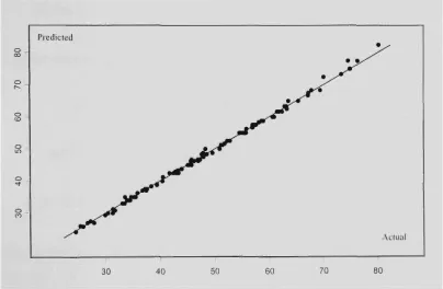
To see the usefulness of the predictions the ASET-B model was run for 100 ran-dom points over the design range and predictions made based on the fitted com-puter model. Figure 2.4 shows that the predictions match the actual responses from ASET-B quite closely.
Figure 2.4: AccuracA- of Prediction for Egress Time
2.6 Interpretation of Results
2.6.1 Analysis of Main Effects and Interactions
CHAPTER 2. ANALYSIS OF A SIMPLE COMPUTER MODEL 33
Sacks et al. (1992) defined, for a computer model Avith input range u € [0.1]*^. the mean, main effects and interaction effects as
Po = / ••• / .?/(u)]^c/u/,
[0,1]'^ ''""' /ii(a,) = ••• y{u)Ylduh- tiQ
l.i,,j{u,,Uj) = •• y{u) Yl '^"'> ~ /''("') ~ ^ j ( " j ) ^
-^^0-[0,1]^ ^ ^ ^ J
For a model defined on z G [—1,1]'^ the definitions become
Mo = T^ / - • • / .?/(z) n ^^^ 2d
- l . l ] " ' ^ = 1
• [ - L l ] " ''^'•^
In practice, the true effects are estimated b}- replacing y{z) hy y{z) in the alxn-e expressions.
Since the BLUP estimator of y is giA-c^n IJA- Eciuation 1.8 then the estimator y can be re-written as:
•y(z) = ;'i + r'^(z)w
AA-liere
w^Kf^ij-lft)
and r(z) is giA-en bA- Eciuation 1.9. Hence y(z) can be CA-aluated as
y{z) = fj + a'ii?(Xi. Z) + U'27?(X2, Z) + . . . + U'„7?(x„. Z)
CHAPTER 2. ANALYSIS OF A SIMPLE COMPUTER MODEL 34
For a 4 dimensional case, as here, consider
1
y(z) dzi dz2 dz'i dz^
- i . i l
1
¥
1
2^
-1.11
.? + J ^ u ; , i ? ( x f c , z ) fc=i
dz\ dzo d::i dzji
^ 1 1 dzj dz2 dz-i dz4
-1.1]^
+ X ^ ll-'k / / / / ^ ( X f c , z) f/2i dz2 dZ:i dz4
^^'^ [-1.1H
^ + ^ E '^'W / / / ^(^'^^ ') '^'^ ^~2 '/^i 'h^
k=l
-hiV
'^+Y^fl'''^- n / exp(-9,\x,,,-z,r)dz,
k=i h = \
Similarlv.
,3 / / / y(^) d--^ ^--i d-^ -1,11^
1
I
1
9^
-1,113
• H ^ » > / ? ( X 4 . . Z )
A = l
f/.:2 d.2:i <I^4
3 dz, dz. dz 3 " - 4 - 1 . 1
A = l
+ 5 ^ (('A. / / / ^(XA-. Z) r/^2 c/-3 dZ4 l-l.lp
^ ((•/,. exp (-6*1 [.Cfci - ^l|^'
H
fc=iCHAPTER 2. ANALYSIS OF A SIMPLE COMPUTER MODEL 35
Finalh-,
22 J J ^^^"^ "^^^ "^^^ " 22
1-1.ip 1
1
ft + ^ li'kRi^k- z) dz:i dz4
-1,1]2 k=l
3 I I dzs dz4
I-i,'iP
+ ^ ^'k / / -R(xfc, z) dzs dz4
k=\
= ^ +
Y^
[ - 1 , 1 P n
X
^ Wk exp ( - ^ 1 |,Tfci - zil"' - 02 [r^.2
k=l
n / e x p ( - . ^ , ] , r , , - 2 , , | ^ " ) c / - / i , _ o 7 - i
-, |P2^ - 2 ,
Note that all these quantities onl}- depend on one-dimensional integrals
/ exp(-^;,|.r hk — ^k\ ) <l^k
where x^]^ is h*'^ component of the A-*^ point of the initial experiment and z^ is the
j^th component of an arbitrarA' point. This is so since the integrand is separable
in
Zh-In general
d „ i
p,(z,,) = .3 +
k=l lj = l-^~^ n
y ^ »'fc exp (-^,- I.Tfcj - Zjl"')
2d-1
,fc=i
X n / ' e x p ( - ^ , | „ r , , - z , r ) c / : hyti--'-'^
A'o (2.7)
/' ( . j \ - ( - ^ , / ,
^^ +
2^-^ y ^ (/'A-exp - 5 ^ ^/il •X/t/i - ^ / i ^ ' ^
,fe=i h=i.j
J l / exp(-^^|.Tfch-2/i|^'0c?2ft 1.1,{Z,) P j ( 2 j ) / ^ o
CHAPTER 2. ANALYSIS OF A SIMPLE COMPUTER MODEL 36
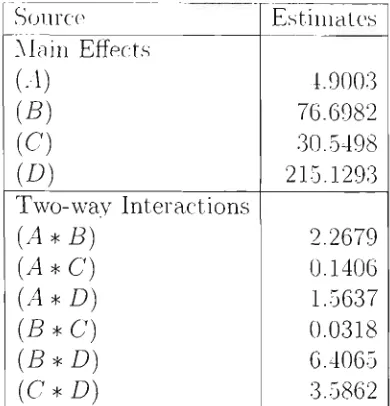
2.6.2 Apphcation t o ASET-B Computer Experiment
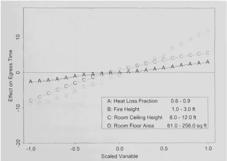
Using the results of the previous .section, estimates of the aA-erage oA-er the ex-perimental region, given by Equation 2.6, and the main effect of input factor x,
(averaged over the other factors), given b}- Equation 2.7. were calculated. Es-timates were obtained by replacing y(z) bv jj{z). The estimated value of po is 48.75. The main effect function is given in Figure 2.5, showing that the Egress Time increases as each of the input factors increases, with the most important factors over the ranges studied being Room Floor Area (D) and Fire Height (B). Heat Loss Fraction (A) and Room Ceiling Height (C) are less important in this model.
0)
E
w
<D
i _
CD
LU c o "o
CD
LU
= 5 = ^
,, r.-C O^
p , - - u
r C- ^ . « a-—A—A—/^
Jl-A-A-_A^A---A'
o A'
C
, A - A - A '
,C
.X'-A:
B:
C
D:
Heat Loss Fraction
Fire Height
Room Ceiling Height
Room Floor Area
0.6
1.0
8.0- 81.0--0.9
-3,0 ft
12.0ft
256.0 sq ft
-1.0 -0.5 0.0
Scaled Variable
0.5 1.0
Figure 2.5: Main Effects plot for the ASET-B Computer Model.
CHAPTER 2. ANALYSIS OF A SIMPLE COMPUTER MODEL 37
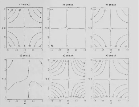
Avere calculated, Avith estimates obtained bv replacing y{z) by y{z). Contours of the interaction functions are given in Figure 2.6. The deviations from additivity are quite small (since the interactions are small relative to main effects). The joint effects of each pair of factors are given in Figure 2.7.
x1 and x2
o\5 p -g 5
•1,0 -0,5 0 0 0,5
x2 and x3
-05 0,0
x1 and x3
-0 5
J
1 ^
3
r
-10 -0,5 0 0 0,5 1,0
x2 and x4
•/s / -V.s J -d5
a M \ ''J' ^ o>5
\
• 0
x1 and x4
^5 \ 0^5
^ ^ 5
•- 0
1 -0/5 / _,4
-0 5 0 0 0 5 to
x3 and x4
-^^^ -V5 J' -q5
S^sV l\5 \ Ols
\ \ \ 5
1 45 / .y{ ^
Figure 2.6: Interaction plot for the ASET-B Computer Model.