The Population Genetics of Clonal and Partially Clonal Diploids

(1)



The Population Genetics of Clonal and Partially Clonal Diploids

Franc¸ois Balloux,*

,†,1

_{Laurent Lehmann}

‡

_{and Thierry de Meeu}

_ˆs

§

*I.C.A.P.B., University of Edinburgh, Edinburgh EH9 3JT, Scotland, United Kingdom,†_{Department of Genetics, University of Cambridge,}

Cambridge CB2 3EH, United Kingdom, ‡_{Institute of Ecology (Zoology and Animal Ecology), University of Lausanne, 1015 Lausanne,}

Switzerland and§_{Centre d’Etude du Polymorphisme des Microorganismes, Equipe ESS, UMR 9926 CNRS-IRD, BP64501,}

34394 Montpellier Cedex 5, France Manuscript received November 6, 2002 Accepted for publication April 11, 2003

ABSTRACT

The consequences of variable rates of clonal reproduction on the population genetics of neutral markers are explored in diploid organisms within a subdivided population (island model). We use both analytical and stochastic simulation approaches. High rates of clonal reproduction will positively affect heterozygosity. As a consequence, nearly twice as many alleles per locus can be maintained and population differentiation estimated asFSTvalue is strongly decreased in purely clonal populations as compared to purely sexual

ones. With increasing clonal reproduction, effective population size first slowly increases and then points toward extreme values when the reproductive system tends toward strict clonality. This reflects the fact that polymorphism is protected within individuals due to fixed heterozygosity. Contrarily, genotypic diversity smoothly decreases with increasing rates of clonal reproduction. Asexual populations thus maintain higher genetic diversity at each single locus but a lower number of different genotypes. Mixed clonal/sexual reproduction is nearly indistinguishable from strict sexual reproduction as long as the proportion of clonal reproduction is not strongly predominant for all quantities investigated, except for genotypic diversities (both at individual loci and over multiple loci).

T

HE essential feature of sexual reproduction is that In another respect, theoretical considerations predict genetic material from different ancestors is brought that the effective population size of clonal organisms together in a single individual. If sexual reproduction is should be lower than that of panmictic ones (e.g.,Orive

dominant in eukaryotic organisms (e.g.,Charlesworth 1993;Milgroom 1996). However, the few theoretical 1989;Westet al.1999), many organisms of major medical population genetics studies that we are aware of provide or economical importance are known to reproduce ambiguous conclusions on that topic (Orive1993;Berg

mainly or strictly clonally (e.g.,Milgroom1996;Taylor andLascoux 2000) and numerous field observations

et al.1999;Tibayrenc1999). The presence or absence support this ambiguity (e.g.,Butlinet al.1998;

Gabri-of a sexual process will crucially determine the genetics _elsen and Brochmann1998;Cywinska and Hebert

at both the individual and the population level and leads _{2002). Thus, “whether organisms with clonal} reproduc-to several straightforward predictions. At the individual _{tion necessarily have lower genetic diversity is unclear”} level, clonality will produce a strong correlation between ₍_Orive_{1993, p. 337). These ambiguities illustrate what} alleles within individuals at different loci, as they share _{little is known on the population genetics consequences} a common history within a clonal lineage. Sex on the _{of clonal reproduction. In the absence of theoretical} other hand will break these associations, allowing for _{models providing clear expectations, estimating the rate} many more potential genetic combinations. Further, in _{of clonal reproduction in natural populations appears} diploids, absence of sex will promote divergence be- _{problematic (}_e.g._,_Anderson_and_Kohn_{1998) and even} tween alleles within loci, as the two copies will accumu- _{the detection of purely clonal populations is often} con-late different mutations over time. This effect has been _{troversial (}_e.g._, _Tibayrenc _1997;_Vigalys _{et al.} _1997). termed the “Meselson effect” and has recently been _{Clonality is not just an academic matter (}_Tibayrenc experimentally documented in bdelloid rotifers, which _{1997). Many diploid organisms believed to reproduce} are believed to have been reproducing strictly clonally _{mainly or strictly clonally are of major medical,} veteri-over long evolutionary time (Butlin 2000; Mark _{nary, and economical importance, including}

patho-Welch and Meselson 2000, 2001). Heterozygosity is _{genic fungi such as Candida or protozoans such as}

Try-thus expected to increase indefinitely under clonal _{panosoma. A better understanding of the reproductive} propagation (Birky1996;JudsonandNormak1996). _{system of such organisms might be crucial for planning}

successful long-term drug administration or vaccination programs (Tibayrencet al.1991;Milgroom1996;

Tay-1_{Corresponding author:}_{Department of Genetics, University of}

Cam-loret al.1999).

bridge, Downing St., Cambridge CB2 3EH, United Kingdom.

E-mail: [email protected] Here we present both analytical and stochastic

(2)

tion results for the population genetics of clonally and FA(t⫹1)⫽ FJ(t⫹1/2)

partially clonally reproducing populations. We focus on _␪

A(t⫹1)⫽ (qs␪J(t⫹1/2)⫹ (1⫺qs)␣J(t⫹1/2))

a simple population subdivision model (island model)

␣A(t⫹1)⫽ (qd␪J(t⫹1/2)⫹(1 ⫺qd)␣J(t⫹1/2)), (1)

and restrict our work to neutral mutations. We derive the identities by descent, F-statistics, and mean

coales-withqsbeing the probabilities that two individuals taken

cence times of alleles and genotypes for variable rates

at random within the same subpopulation after migra-of clonal reproduction. We also investigate the allelic

tion were born in the same deme. The exact expression and genotypic diversities maintained under different

forqsis relatively cumbersome (seeWang1997).

How-rates of clonal reproduction.

ever, for relatively large values of N, qsreduces to the

much more compact form that we use throughout the article,

MODEL ASSUMPTIONS AND GENETIC IDENTITIES

qs⬵(1⫺m)2⫹

(m)2

n ⫺1, (2)

We consider a subdivided monoecious population of diploid individuals, which reproduce clonally with

prob-wheremrepresents the migration rate andnthe number abilityc, with sexual reproduction occurring at the

com-of subpopulations. Now we can defineqdas the

probabil-plementary probability (1 ⫺ c). Sexual reproduction

ity that two individuals sampled after migration in differ-in the model follows random union of gametes,

self-ent subpopulations originated from the same deme: fertilization occurs at a rate s, and a subpopulation is

composed ofNnumber of adults. In our model,

individ-qd⫽

1⫺ qs

n⫺ 1. (3)

uals, rather than gametes, migrate following an island model (Wright1951) at a ratem, implying that a

mi-We then express juvenile identities as functions of adult grant has an equal probability to reach any of the

sub-identities in the previous generation. Here both muta-populations. We further assume stable census sizes and

tion and the reproductive system will affect the genetic population structure and no selection. The life cycle

identities of juveniles. The mutation rate is u for all involves nonoverlapping generations and juvenile

mi-alleles and therefore the probability of two mi-alleles that gration. The precise sequence goes as follows:

are identical by descent before mutation still being iden-tical after mutation will be␥⬅(1⫺u)2_{. In the absence}

1. Adult reproduction and subsequent death

of any mutation event, clonal reproduction occurring 2. Juvenile dispersal

at ratecwill produce offspring identical to its progeni-3. Regulation of juveniles, the survivors reaching

adult-tor, so that the inbreeding coefficient of a clonally pro-hood

duced juvenile individual will be identical to its parent’s. Because of the symmetry of the island model, only _{Selfing occurs with probability} _s_{, and in that case the} the following probabilities of identity by descent are coancestry will be (1⫹FA)/2. With a probability 1⫺s,

needed to describe the apportionment of genetic varia- nonselfing sexual reproduction occurs, the offspring tion in a subdivided monoecious population. will have two parents, and its inbreeding will be the parental coancestry (␪A). This gives us the following

F: The inbreeding coefficient, defining the probability _{juvenile identities as functions of adult identities:} that two alleles drawn at random from a single

indi-vidual are identical by descent. _F

J(t⫹1/2)⫽ ␥

冢

c FA(t)⫹(1⫺c)

冢

s

冢

1 ⫹FA(t)

2

冣

⫹(1⫺s)␪A(t)

冣冣

␪: Coancestry of individuals drawn at random from

within the same subpopulation, defined as the

proba-␪J(t⫹1/2)⫽ ␥

冢

1

N

冢

1⫹FA(t)

2

冣

⫹

冢

1⫺ 1

N

冣

␪A(t)

冣

bility that two randomly sampled alleles from two different individuals within a subpopulation are

␣J(t⫹1/2)⫽ ␥(␣A(t)). (4)

identical by descent.

␣: Coancestry of individuals randomly drawn from dif- _{Substituting Equation 4 in (1), we obtain the recurrence} ferent populations. This is defined as the probability _{equations for describing the dynamics of identities} that two randomly sampled alleles from two individu- _{among adults:}

als in different subpopulations are identical by

de-scent. _F

A(t⫹1)⫽ ␥

冢

冢

(3)

The recurrence equations for␪Aand␣Aare identical to individuals relative to randomly drawn gametes from

the entire population. In more biological terms FIS is

those given byRousset(1996, Equation 2). OnlyFAis

affected by the variable amount of clonal reproduction interpreted in terms of deviation from random mating, caused by the breeding system of the organism under and by the fact that we assume zygotic rather than

ga-metic migration. study, and FST represents the heterozygote deficiency

due to population subdivision. FinallyFITis the measure

For analytical effectiveness, recurrence equations for

identities by descent can be presented in matrix form, of inbreeding taking into account both deviations from random mating within subpopulations and the effects of

Q(t⫹1)⫽ ␥GQt⫹ ␥D, (6)

population subdivision. The relation linking the three coefficients can be expressed as

whereQtis a column vector of the probabilities of identi-ties at generationt⫹1. The transition matrixGdefines

(1 ⫺FIT)⫽(1 ⫺FST)(1⫺FIS) (9)

the probabilistic changes of the vector variables, andD

is the constant column vector. Solving (6) at equilibrium (CrowandKimura1970, p. 106).

we obtain the identities from Within-population deviations from random mating (FIS):Replacing the solutions of Equation 7 in (8), we

Q⫽ ␥(I⫺ ␥G)⫺1_D ₍₇₎

getFISafter migration for subdivided populations with

a mixed system of clonal and sexual reproduction withIbeing the identity matrix.

(selfing set to 1/N) and zygotic migration

FIS⫽ ␥

(qs⫺c(␥(qs⫺qd)⫺1)⫺1)

2N(1⫺ ␥c)(␥(qs⫺qd)⫺1)⫺ ␥(qs⫺c(␥(qs⫺qd)⫺1)⫺1) .

INDIVIDUAL-BASED SIMULATIONS

(10) To obtain the variances of the quantities of interest, as

well as multilocus behavior, we additionally performed

Neglecting mutation (␥ ⫽1), but allowing for a mixed stochastic individual-based simulation, as implemented

system of clonal reproduction with arbitrary selfing rate, in the software EASYPOP (version 1.7.4;Balloux2001).

we obtain For all simulations, we used 20 loci with a mutation

rate of 10⫺5_{. Mutations had an equivalent probability to}

FIS⫽

Nn(1⫺c)s⫺ 1

Nn(1⫺ c)(2⫺s)⫹1

. ₍₁₁₎

generate any of the 99 possible allelic states. This rela-tively high number of allelic states keeps the probability

The equation shows thatFISis independent of the

migra-of obtaining indistinguishable alleles through different

tion rate but sensitive to the total number of individuals mutational events (homoplasy) low. At the start of the

in the population; this occurs because we assumed zy-simulation, genetic diversity was set to the maximum

gotic rather than gametic migration. Under random possible value at the first generation and the simulation

mating (s⫽1/N) we further obtain was then run for 10,000 generations, the point at which

all statistics measured in EASYPOP (FIS,FST,HS,HT, and

FIS⫽

(1⫺c)n⫺ 1

(1⫺ c)(2N⫺ 1)n⫹ 1. (12) the number of alleles) had reached equilibrium. All

simulations were replicated 20 times.

When reproduction is strictly sexual (c⫽0), Equation 12 reduces to the form

F-STATISTICS

Deviations from random mating are generally ex- FIS⫽

n⫺ 1

(2N⫺1)n⫹1. (13) pressed by means of F-statistics (Wright 1951). They

are the most commonly used tools for describing gene _{For a strictly clonal population (}_c_⫽_1),_F

IS⫽ ⫺1. This

flow and breeding structure in both theoretical and _{reflects the fact that in the absence of sexual} reproduc-empirical studies (reviewed in Balloux and Lugon- _{tion, all individuals are expected to be heterozygous at}

Moulin2002). F-statistics are defined as _equilibrium_F _⫽_{0, while}_{␪ ⫽}1_⁄

2.

In Figure 1, we plotFISas obtained from Equation 10

FIS ⫽

F⫺ ␪

1⫺ ␪, FST⫽ ␪ ⫺ ␣1⫺ ␣, FIT⫽

F ⫺ ␣

1⫺ ␣ (8) against the rate of clonal reproduction. We also give values obtained from individual-based simulations. Ana-lytical and stochastic simulation results are in excellent

(Cockerham 1969, 1973), where subscripts I, S, and

T represent individuals, subpopulations, and the total agreement. From Figure 1, it can be seen that for very high values of clonal reproduction, huge heterozygote population, respectively.FIScan be thought of as a

mea-sure of the identity of alleles within individuals relative excesses are obtained. However, as long as there is a small proportion of sexual reproduction,FISstays close

to the identity between alleles randomly drawn from

two different individuals from within the same subpopu- to what is expected under panmixia; a significant excess of heterozygotes occurs only for extreme rates of asexu-lation.FSTis the identity of alleles drawn randomly from

within a subpopulation relative to alleles drawn from ality. As long as there is mutation in the system, FIS

(4)

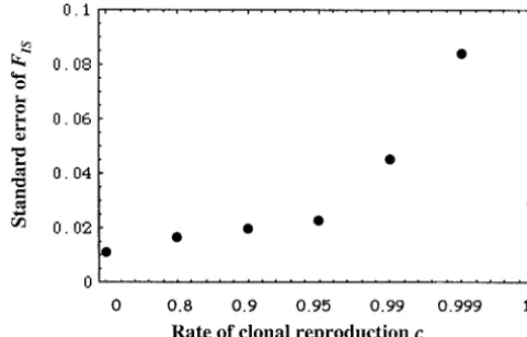
Figure1.—FISas a function of the rate of clonal reproduc- Figure2.—Standard errors ofF_ISas a function of the rate

tion. Parameter values are as follows: number of populations, _{of clonal reproduction. The standard errors are computed on} n⫽50; number of individuals per population,N⫽50; migra- _{20 physically unlinked loci. The simulation parameter values} tion rate,m⫽0.1; mutation rate,u⫽10⫺5_{; selfing rate is set}

are as follows: number of populations, n ⫽ 50; number of to random mating, s⫽1/N. The line represents analytical _{individuals per population,}_N_⫽_{50; migration rate,}_m_⫽_0.1; results and the solid circles simulation results. _{mutation rate,}_u_⫽₁₀⫺5_{; selfing rate is set to random mating,}

s⫽1/N.

of the number of individuals in the complete population

(nN) times the mutation rate is high, theFISvalue for The amount of clonal reproduction has a strong effect

complete clonality can be very much offset from ⫺1. _{on population differentiation. Whereas even for very} The reason for this can be seen from Equation 8. Under _{limited proportions of sex, there is no noticeable effect,} clonal reproduction all individuals will be heterozygous _{when reproduction tends toward strict clonality,} _F_ST _is and this will not be changed by mutation, so F ⫽ 0, _{strongly reduced. Note that in the absence of any} muta-while␪ decreases with increasing mutation rate. _tion,_F_ST_{would be defined but equal to 0, as all the genetic} The FIS estimates from the stochastic simulations in variance is within individuals and none between

individ-Figure 1 are averaged over loci and replicates and do uals and subpopulations. In all simulated cases the be-not reveal anything about the strong influence of the tween-loci variance of FST strongly increases with the

rate of clonal reproduction on the variance over loci. proportion of clonal reproduction (results not shown). This huge variation among loci, in particular for low

rates of sexual reproduction, is illustrated by standard

EFFECTIVE POPULATION SIZE errors in FIS (Figure 2). The lowest variations are

ob-tained with pure clonality and with⬍95% of clonality. _{Effective population size:} _{The effective population}

Population differentiation (FST):Again by replacing _{size (}_Wright_{1931) is the parameter summarizing the}

the solutions of Equation 7 in (8), we obtain FST for _{amount of genetic drift to which a population is}

sub-subdivided populations with a mixed system of clonal, _{jected. It is quantified as the number of idealized} ran-selfing, and sexual reproduction after migration: _{domly mating individuals that experience the same}

amount of random fluctuations at a neutral locus as the

FST⫽ ␥(1⫺

c␥)(qs⫺qd)

N(1⫺ ␥(qs⫺qd))(2⫹c(s⫺2)␥ ⫺s␥)⫹ ␥(qd(␥(c⫹1)⫺1)⫺qs(␥(c⫹1)⫺2))

.

population under scrutiny. The dynamics of idealized (14)

randomly mating individuals are described by the Wright-Fisher model, whose well-known properties lead to dif-Neglecting mutation (␥ ⫽1) leads to

ferent definitions of the effective population size de-pending on whether the quantities of interest are the

FST ⫽

(1⫺c)(qs⫺qd)

N(1⫺c)(2⫺s)(1⫺(qs⫺qd))⫹c(qd⫺qs) ⫹qs

.

variance of change in allelic frequencies, inbreeding (15) _{coefficients, or the rate of decline in heterozygosity}

(Ewens1982;WhitlockandBarton1997). Here we

Finally, if only sexual reproduction is allowed (c ⫽ 0

introduce a new definition of effective size called the ands⫽1/N), we get

coalescence effective size,

FST⫽

(qs⫺qd)

(2N⫺ 1)(1⫺ (qs⫺qd))⫹ qs

. ₍₁₆₎

Ne⫽

1

2t, (17)

In Figure 3, we plotFSTas obtained from Equation 14

(5)

into Equation 19, a closer look reveals that the vector

Qdefines the probability-generating functions of coales-cence time at each level i. These functions reduce to the calculations of expected coalescence times as

ti ⫽

⳵Qi

⳵␥

兩

␥⫽1, (21)

wheretiis the expected coalescence time at leveliand Qiis theith row of the equilibrium vector given by

Equa-tion 20 and their variances as

␴2₍_t i)⫽

冤

⳵2_Q i

⳵␥2 ⫹

⳵Qi

⳵␥ ⫺

冢

⳵Qi

⳵␥

冣

2

冥

␥⫽1

. (22)

Figure3.—FSTas a function of the rate of clonal reproduc- _{At this point we have all necessary tools to obtain the}

tion. Parameter values are as follows: number of populations,

mean coalescence times of alleles in a subdivided popu-n ⫽ 50; number of individuals per population, N ⫽ 100;

lation with arbitrary rates of clonal reproduction. Writ-migration rate,m⫽10⫺2_{; mutation rate,}_u_⫽₁₀⫺5_{; selfing rate}

ing the recurrence equations (5) under the form given is set to random mating,s⫽1/N. The line represents analytical

results and the solid circles simulation results. in Equation 18 and using Equation 21 yields the follow-ing mean coalescence times,

tF⫽

2(1⫹(1⫺c)nN(1⫺s)) 1⫺c

ancestor. For the Wright-Fisher modelt ⫽2N, so that the effective size reduces to the actual number of diploid individuals. This definition of effective size allows us to _t

␪⫽1⫹(1⫺c)nN(2⫺s)

1⫺c disentangle the allelic effective size (all classical

defini-tions) from the genotypic effective size (see below), and

t␣⫽n⫺1

2m ⫹

4⫹(1⫺c)n(3⫹4n(2⫺s)) 4(1⫺c) ⫹

n2_m

8(n⫺1), we can further obtain their variance.

There is a strict relationship between identity-by-descent ₍₂₃₎

probabilities and coalescence times (Slatkin 1991;

Rousset1996). The probability of identity of any pair wheret␣ is a low migration limit obtained by a

first-of alleles is the probability that neither allele has under- degree Taylor expansion. The mean coalescence time gone mutation since their most recent common ances- of two randomly sampled alleles is the expectation of tor (Hudson1990). Recalling Equation 7, theti; in the finite-island model this yields

Q⫽ ␥(I⫺ ␥G)⫺1_D_. ₍₁₈₎

t⫽ 1 n

冢

1

NtF⫹

冢

1⫺

1

Substituting Equation 24 into (17), we obtain the coales-of the matrix G as D ⫽ 兺jajrj, wherej is the number

cence effective population size. Note that this effective of columns ofG, aj the coefficient determined by the

size captures the loss of allelic diversity in the population preceding system of equations, andrj ⬅ (r1j, . . . ,rkj)T

and we refer to it as 2Ne, the allelic effective population

thejth right eigenvector ofG. Using the fact that the

size, which is equal tot in our model. In Figure 4, we

jth eigenvalue of the matrix (I⫺ ␥G)⫺1_{is 1/(1}⫺ ␥␭ j),

plot the effective population size as a function of clonal and its associated right eigenvector is rj, where ␭j is

reproduction and selfing rate (the union of gametes the jth eigenvalue of G, we can express Equation 18

within individuals). Increasing the rate of clonal repro-followingRousset(2002) as

duction has no noticeable effect on most of the parame-ter space. However, when the reproductive system tends

Q⫽

兺

j

␥ajrj

1⫺ ␥␭j

⫽

_兺

∞

t⫽1

␥t

兺

j

␭t⫺1

j ajrj. (19)

toward complete asexual reproduction, the effective pop-ulation size suddenly tends toward infinite values. This The second equality is obtained by using the property

slightly counter-intuitive result simply reflects that the of geometric series. Then

genetic diversity within individuals cannot be lost in clonal organisms. Doubling ofNecompared to random

ci(t)⫽

兺

j

␭t⫺1

j ajrij (20)

mating is observed approximately when the rate of sex-ual reproduction is in the order of 10⫺4_{with the}

simula-is the coalescence probability of alleles at timetat any

tion parameters used in Figure 4. Contrarily, increased hierarchical leveli(whereistands forF,␪, and␣). From

rates of selfing decrease effective population size. This this, we can obtain the expected coalescence times by

(6)

⫹(N⫺1)(N⫺2)

N2 ⌬(t)

冣

⫹(1⫺c)2

冢

1

4N2⫹

3 4N3F(t)⫹

2((2N)2_⫺₁₎

(2N)3 ␪(t)⫹

4(2N⫺1)(2N⫺2) (2N)3 ␳(t)

⫹(2N⫺1)(2N⫺2)(2N⫺3)

(2N)3 ⌬(t)

冣

. (25)

Note that whenc⫽0,F⫽ ␪, and the recurrence equa-tions reduce toCockerham’s (1971) model. Substitut-ing these equations into a transition matrix G and a column vector of constants D following Equation 18 allows us to obtain the mean coalescence times:

tF⫽

2(c⫹ N(1⫺ c)) 1⫺ c

Figure4.—Effective population size as a function of selfing

(front axis) and clonal reproduction (right axis). Parameter

values are as follows: number of populations,n⫽50; number t␪⫽c ⫹2N(1 ⫺c)

1⫺c

of individuals per population,N⫽100; migration rate,m⫽0.1.

t␳⫽N(8N ⫹2c

2₍_N ⫺₁₎⫹ _c₍₉⫺ ₁₀_N₎⫺ ₃₎

(1⫺c)(3N ⫺c(N ⫺1)⫺1) betweenNeunder absence of selfing to Ne/2 for strict

selfing.

Genotypic and allelic effective population size: We t⌬⫽

冦

c3_a

0⫹c2a1⫹ca2⫹ a3

c3_b

0⫹c2b1⫹cb2⫹ b3

, c⬆1

N, c⫽1. (26)

have shown that increased rates of clonal reproduction will increase the allelic effective population size, and

t⌬is the mean coalescence time for genotypes and we

thus clonal populations are expected to maintain more

refer to it as the genotypic effective size. This quantity alleles at neutral loci than are sexually reproducing

is undefined forc⫽1 as the matrixGis not diagonaliz-ones. We can go a step further and address the issue

able in this case. However, we know that when c ⫽ 1, of how clonal reproduction will affect the number of

the genotypic identity is independent ofF,␪, and␳and different genotypes maintained. The coalescence

ap-thus follows a dynamic similar to haploid genetics, with proach allows us to capture qualitatively these trends

mean coalescence timeN. Whenc⬆1, the mean geno-by calculating the genotypic effective population size. To

typic coalescence timet⌬takes the form of a relatively

obtain this quantity, we need, in addition toFand␪,␳,

complex polynomial (the coefficients are given in

ap-the probabilities that three alleles randomly sampled

pendix b). Note that in the absence of clonal

reproduc-in two different reproduc-individuals are identical. These three

tion, there is a very compact approximation for the variables are necessary to calculate the probability ⌬

genotypic coalescence timet⌬⬇3N (seeappendix b).

that two genotypes are identical. However, these

higher-Mean coalescence time for alleles in a nonsubdivided order coefficients are complicated and we therefore

population can be obtained ast⫽(1/N)tF⫹ (1⫺ 1/

limit ourselves to a non-subdivided monoecious

popula-N)t␪and thus reads

tion without mutation. We follow the approach of

Cock-erham(1971, pp. 243–244) to calculate the dynamics

of these four variables. Collecting the identities given in t⫽c(1⫹N)⫹ 2N

2₍₁⫺_c₎

N(1⫺ c) . (27)

appendix aleads to the following system of recurrence

equations: _{Note that we could have obtained the allelic effective} size directly from Equation 24 assuming no migration, F(t⫹1)⫽c F(t)⫹(1⫺c)

冢

1

␪(t) genotypes. It can be seen that contrarily to what is ob-served at the allelic level, genotypic effective size

de-␳(t⫹1)⫽c

冢

1

NF(t)⫹ N⫺1

N ␳(t)

冣

creases with increasing clonality. The decrease is rela-tively smooth over the complete parameter range of c

and reachesN for strict clonality. The intuitive reason

⫹(1⫺c)

冢

1

N2

冢

1 4⫹

3 4F(t)

冣

⫹

⫹

3(N⫺1)

N2

冢

1 2␪(t)⫹

1 4␳(t)⫹

1

(7)

Figure5.—Allelic effective population size (solid line) and genotypic effective population size (dashed line) in a non-subdivided population. The values given are for a population

Figure6.—Effective number of alleles (solid circles) and

of 20 individuals.

genotypes (open circles) as functions of the rate of clonal reproduction. The effective number of genotypes is computed for 20 physically unlinked loci. Parameter values are as follows: GENETIC DIVERSITIES _{number of populations,}_n_⫽ _{50; number of individuals per} population,N⫽100; migration rate,m⫽10⫺3_{; mutation rate,}

We can now take a closer quantitative look at how

u⫽10⫺5_{; selfing rate is set to random mating,}_s_⫽_1/N.

genetic diversity is distributed between alleles and geno-types with the stochastic simulations. Allelic diversity

can be expressed as the effective number of alleles,ne, _{all other quantities investigated are significantly affected}

corresponding to the number of equally frequent alleles _{only when sexual reproduction becomes rare.}

needed to observe a given genetic diversity, which is 1/ _{Our results thus suggest that strict clonality may easily} (兺pi2), wherepiis the frequency of theith allele. Simi- _{be detected in diploid populations due to heterozygote}

larly, we can express the effective number of genotypes _{excess. Furthermore, very low levels of sex (cryptic sex)} asGe ⫽ 1/(兺gi2), where gi is the frequency of the ith _{may also be revealed by on average low}_F

IS values with

genotype. In Figure 6 we plot both the effective number _{very important variance among loci, though DNA} alter-of alleles and genotypes within a subpopulation. The _{ations may also lead to a similar pattern in a strictly} number of alleles maintained is strongly positively af- _{clonal population. For instance,}_{Candida albicans}_{is known} fected when the reproductive system tends to be com- _{to undergo mitotic recombinations including} chromo-pletely asexual. This effect is generated by fixed hetero- _{somal translocation (}_Lott_{et al.}_{1999). Much effort has} zygosity (i.e., under strict clonal reproduction in diploids _{been put into testing for evidence of strict clonal} re-the two alleles at each locus are behaving as two haploid _{production with traditional population genetics (}_e.g_., loci). In contrast to allelic diversity, clonal reproduction _Tibayrenc_{et al.}_{1991) or through testing for the} Mesel-decreases the effective number of genotypes steadily _{son effect (high divergence at the two alleles of a single} (Figure 6). To summarize, populations of clonal or sub- _{locus within individuals; reviewed in}_Butlin_2000). Ex-clonal organisms can maintain more allelic diversity at _{treme genetic divergence at single loci within} individu-each single locus but fewer distinct multilocus geno- _{als has been documented in bdelloid rotifers, which}

types. _{are believed to be ancient asexuals (}_{Mark Welch}_and

Meselson2000, 2001). The Meselson effect could,

how-ever, not be detected in other potentially old asexual DISCUSSION

lineages (Scho¨ net al. 1998;Normark1999). Whether this is due to rare sex or perhaps to extremely frequent We used both an analytical approach and stochastic

individual-based simulations to describe the dynamics gene conversion events (the copy of the DNA sequence of one chromosome on the other) is an unresolved issue of genetic variance in subdivided populations,

charac-terized by various levels of clonal reproduction. Higher to date.

Empirical data on genetic variation and its apportion-rates of asexual reproduction will increase

heterozygos-ity and decrease population differentiation. Diversheterozygos-ity at ment by means ofF-statistics in clonal lineages, as com-pared to sexually reproducing populations of the same single loci will be higher in clonal organisms than in

sexuals, whereas the opposite is true for genotypic diver- species, are rare. Furthermore, studies using dominant genetic markers (e.g., rapidly amplified polymorphic sity. At the exception of genotypic diversity (both at single

(8)

types. Indeed, as can be seen from Figure 6, the absolute tively robust to reasonable differences in relative fitness genetic diversity (the sum of allelic and genotypic vari- between clonally and sexually produced offspring. ability) does not provide any clear prediction on the Finally, our model could lead to the development of rate of clonal reproduction. Another potential problem new approaches to infer the rate of clonal reproduction. stems from the difficulty in ruling out the presence of Our results show that all estimators based on identities rare sexual reproduction. However, a recent study by by descent (including linkage disequilibrium approaches)

Delmotte et al. (2002) comparing eight sexual with are expected to be rather insensitive to the rate of clonal

five asexual populations of the aphidRhopalosiphum padi reproduction as long as it does not become strongly could provide a test for our model. Their empirical predominant. It is therefore doubtful that such estima-results are overall in good agreement with our analytical tors will allow precise inferences on the actual rate of expectations. As we expect,Delmotteet al.(2002) re- clonal reproduction unless it is very close or equal to port increased excess in expected heterozygotes (FIS) for 1. As genotypic diversity decreases smoothly with the

asexuals and lower differentiation (FST) between asexual rate of clonal reproduction, one promising alternative

populations than between sexual populations. They also approach would be to build estimators of clonal repro-report lower genotypic variation and lower allelic varia- duction as functions of the relative genotypic and allelic tion in asexuals than in sexuals. This relatively good identities.

agreement between our model and their data suggests _{We thank Nathalie Charbonnel, Sylvain Gandon, Jero}_{ˆme Goudet,} that these asexual populations have not experienced _{Andy Overall, Franck Prugnolle, Franc¸ois Renaud, Max Reuter, Denis} sexual reproduction in recent times. The discrepancy Roze, Michel Tibayrenc, and two anonymous referees for very inspir-ing conversations and comments; Franc¸ois Rousset for havinspir-ing given

in allelic diversity could be due to different factors (e.g.,

access to unpublished material; and Sylvain de l’He´rault for his strong

sampling, extinction-recolonization dynamics).

How-support. F.B. was supported by the Biotechnology and Biological

Sci-ever, even if we assumed all else being equal between

ences Research Council and by grant 823A-067616 from the Swiss

the sexual and asexual aphid populations, selection _{National Science Foundation.} could still reduce genetic diversities more effectively in

the asexual populations. Mutations under strong direc-tional selection make linked loci behave as if they were

LITERATURE CITED evolving under smaller effective population sizes (

Rob-ertson1961). Due to the complete absence of recombi- Anderson, J. B., andL. M. Kohn, 1998 Genotyping, gene

genealo-gies and genomics bring fungal population genetics above

nation in strictly clonal organisms, any strongly

deleteri-ground. Trends Ecol. Evol.13:444–449.

ous dominant mutation will drive the lineage, where it _{Balloux, F}_{., 2001} _{EASYPOP (Version 1.7): a computer program} appeared, to extinction. New beneficial mutations will for population genetics simulations. J. Hered.92:301–302.

Balloux, F., andN. Lugon-Moulin, 2002 The estimation of

popula-also reduce the effective population sizes of clones, as

tion differentiation with microsatellite markers. Mol. Ecol.11:

lineages with a new beneficial mutation will displace _155–165.

other lineages. Berg, L. M., andM. Lascoux, 2000 Neutral genetic differentiation in an island model with cyclical parthenogenesis. J. Evol. Biol.

Indeed our model does not include natural selection,

13:488–494.

so that our results apply strictly to neutral genetic vari- _{Birky, Jr., C. W}_{., 1996} _{Heterozygosity, heteromorphy, and} phyloge-ability or more generally to relatively weakly selected netic trees in asexual eukaryotes. Genetics144:427–437.

Butlin, R. K., 2000 Virgin rotifers. Trends Ecol. Evol.15:389–390.

polymorphisms subject to genetic drift. Genetic drift is

Butlin, R. K., I. Scho¨ nandK. Martens, 1998 Asexual reproduction

the main force driving allele frequencies as long as the _{in nonmarine ostracods. Heredity}_81:_473–480.

selection differential s between alleles is not much Charlesworth, B., 1989 The evolution of sex and recombination. Trends Ecol. Evol.9:264–267.

above the inverse of effective population size (1/Ne).

Cockerham, C. C., 1969 Variance of gene frequencies. Evolution

For higher selection differentials, the effect of genetic _23:_72–84.

drift becomes negligible. However, our predictions Cockerham, C. C., 1971 Higher order probability functions of iden-tity of alleles by descent. Genetics69:235–246.

should hold even for relatively important selection

dif-Cockerham, C. C., 1973 Analysis of gene frequencies. Genetics74:

ferentials in clonal and nearly clonal organisms, as the

679–700.

efficacy of selection acting simultaneously at linked sites _{Crow, J. F}_{., and}_{M. Kimura}_{, 1970} _{An Introduction to Population} Genet-is considerably reduced (HillandRobertson1966). ics Theory. Harper & Row, New York.

Cywinska, A., andP. N. D. Hebert, 2002 Origin of clonal diversity

We assumed identical fitness (in both mean and

vari-in the hypervariable asexual ostracode. J. Evol. Biol.15:134–145.

ance) for clonally and sexually produced offspring. The _{Delmotte, F., N. Leterme, J. P. Gauthier, C. Rispe}_and_{J. C. Simon}_, rate of clonal reproduction is not a heritable trait in 2002 Genetic architecture of sexual and asexual populations of the aphid Rhopalosiphum padi based on allozyme and

microsatel-our model, as it is a fixed property of the population

lite markers. Mol. Ecol.11:711–723.

(clonally produced individuals do not have a higher _{Ewens, W. J}_{., 1982} _{On the concept of the effective population size.} chance to reproduce clonally themselves). Therefore, Theor. Popul. Biol.21:373–378.

Gabrielsen, T. M., andC. Brochmann, 1998 Sex after all: high

different fecundities for sexually or clonally produced

levels of diversity detected in the arctic clonal plantSaxifraga

offspring would result only in increasing the variance

cernuausing RAPD markers. Mol. Ecol.7:1701–1708.

in reproductive success and thus would decrease the _{Hill, W. G}_{., and}_{A. Robertson}_{, 1966} _{The effect of linkage on limits}

to artificial selection. Genet. Res.8:269–294.

(9)

qualita-Hudson, R. R., 1990 Gene genealogies and the coalescent process. _{sampled with probability}_c2_{; the four genes stem either} Oxf. Surv. Evol. Biol.7:1–44.

from the same parent or from two different ones. The

Judson, O. P., andB. B. Normak, 1996 Ancient asexual scandals.

Trends Ecol. Evol.11:41–46. identity between genotypes and three alleles reads

Lott, T. J., B. P. Holloway, D. A. Logan, R. FundygaandJ. Arnold, 1999 Towards understanding the evolution of the human

com-⌬t⫹1 ⫽

1

N⫹

冢

1⫺

1

N

冣

⌬t mensal yeast Candida albicans. Microbiology145:1137–1143.

Mark Welch, M. D., andM. S. Meselson, 2000 Evidence for the evolution of bdelloid rotifers without sexual reproduction or

genetic exchange. Science288:1211–1215. _␳ t⫹1⫽

1

NFt ⫹

冢

1⫺

1

N

冣

␳t (A1)

Mark Welch, M. D., andM. S. Meselson, 2001 Rates of nucleotide substitution in sexual and anciently asexual rotifers. Proc. Natl.

Acad. Sci. USA98:6720–6724. _{(two from one offspring, the third from the other).}

Milgroom, M. G., 1996 Recombination and the multilocus structure

When one offspring is produced clonally and one

of fungal populations. Annu. Rev. Phytopathol.34:457–477.

Normark, B. B., 1999 Evolution in a putatively ancient asexual aphid through random mating, the identity among three

al-lineage: recombination and karyotype change. Evolution 53: _{leles will differ if two or only one allele stem from the}

1458–1469.

clonal offspring, the former case occurs with probability

Orive, M. E., 1993 Effective population size in organisms with

com-plex life-histories. Theor. Popul. Biol.44:316–340. c(1 ⫺ c) and the identity is as in Equation A1. The

Robertson, A., 1961 Inbreeding in artificial selection programmes. _{second case also occurs with probability}_c₍₁ _⫺ _c_{), and} Genet. Res.2:189–194.

the three genes then all stem from the same parent with

Rousset, F., 1996 Equilibrium values of measures of population

probability P3 _{and share identity} ␳3_{. The three genes} subdivision for stepwise mutation processes. Genetics142:1357–

1362. _{might as well stem from two different parents with}

prob-Rousset, F., 2002 Inbreeding and relatedness coefficients: What do

abilityP21 _{and then have identity}␳21_{; finally, they can} they measure? Heredity88:371–380.

stem from three different parents with probabilityP111

Slatkin, M., 1991 Inbreeding coefficients and coalescence times.

Genet. Res.58:167–175. _{and their identity is} ␳111_{. The three types of identities}

Scho¨ n, I., R. K. Butlin, H. I. GriffithsandK. Martens, 1998 Slow

can be expressed as

molecular evolution in an ancient asexual ostracod. Proc. R. Soc. Lond. Ser. B265:235–264.

Taylor, J. W., D. M. Geiser, A. BurtandV. Koupopanou, 1999 The _␳3 t⫹1 ⫽

1 4⫹

3 4Ft, ␳

21 t⫹1⫽

1 2␪t ⫹

1 2␳t, ␳

111 t⫹1 ⫽ ␳t. evolutionary biology and population genetics underlying fungal

strain typing. Clin. Microbiol. Rev.12:126–146.

(A2.1)

Tibayrenc, M., 1997 Are Candida albicans natural populations sub-divided? Trends Microbiol.5:253–254.

For the identity between genotypes, we have with

proba-Tibayrenc, M., 1999 Toward an integrated genetic epidemiology

bility 2c(1 ⫺c):

of parasitic protozoa and other pathogens. Annu. Rev. Genet.

33:449–477.

Tibayrenc, M., F. Kjellberg, J. Arnaud, B. Oury, F. Bre´nie`reet

⌬3 t⫹1⫽

1 2⫹

1 2Ft, ⌬

21 t⫹1⫽

1 2␪t⫹

1 4␳t⫹

1 4⌬t, ⌬

111 t⫹1⫽ ⌬t. al., 1991 Are eukaryotic microorganisms clonal or sexuals? A

population genetics vantage. Proc. Natl. Acad. Sci. USA88:5129–

(A2.2)

5133.

Vigalys, R., Y. Gra¨serandW. Presber, 1997 Response from Vigalys

When we sample two offspring issued from random

et al. Trends Microbiol.5:254–256.

Wang, J., 1997 Effective size andF-statistics of subdivided popula- _{mating with probability (1} ⫺ _c₎2_{, the identities for} ␳ tions I. Monoecious species with partial selfing. Genetics 146:

are given by Equation A2.1. The genotypic identity is

1453–1463.

obtained by summing⌬4_, _⌬22_, _⌬31_,_⌬211_{, and} _⌬1111_{, each}

Weir, B. S., andC. C. Cockerham, 1969 Pedigree mating with two

unlinked loci. Genetics61:923–940. _{identity weighted by its corresponding probability} _P4_,

West, S. A., C. M. LivelyandA. F. Read, 1999 A pluralist approach

P22_,_P31_,_P211_{, and}_P1111_{. The five identities are written} to sex and recombination. J. Evol. Biol.12:1003–1012.

Whitlock, M. C., andN. H. Barton, 1997 The effective size of a

subdivided population. Genetics146:2427–2441. _⌬4 t⫹1⫽

1 4⫹

3

4Ft, ⌬

22 t⫹1⫽

1 12⫹

4 12␪t⫹

4 12␳t⫹

3 12⌬t,

Wright, S., 1931 Evolution in Mendelian populations. Genetics16:

97–159.

Wright, S., 1951 The genetical structure of populations. Ann.

Eu-⌬31 t⫹1 ⫽

1 2␪t⫹

1 2␳t, ⌬

211 t⫹1⫽

1 6␪t ⫹

2 6␳t⫹

3 6⌬t,

gen.15:323–354.

Communicating editor: M. K.Uyenoyama

⌬1111

t⫹1 ⫽ ⌬t. (A3)

The different probabilities of gamete origins are given APPENDIX A: GENOTYPIC PROBABILITIES OF _in_Weir_and_Cockerham_{(1969) and read as}

IDENTITIES BY DESCENT

We follow the same rationale asCockerham(1971, pp. 242–243), but add the dynamics of ␪. When one

P3_⫽ 1 N2, P

21_⫽3(N⫺1)

N2 , P

111_⫽(N⫺1)(N⫺2)

N2 ,

P4_⫽ 1 N3, P

22_⫽3(N⫺1)

N3 , P

31_⫽4(N⫺1) N3 ,

P211_⫽6(N⫺1)(N⫺2)

N3 , P

1111_⫽(N⫺3)(N⫺2)(N⫺1)

N3 .

offspring is produced clonally, his two alleles are not independent. When we sample alleles and look back to their common parent, the two genes of a clone always

(10)

APPENDIX B: COEFFICIENT OF EQUATION 23 _b₃ _⫽₃₆_N3⫺ ₄₅_N2 ⫹₂₀_N⫺_3. _(B1.2)

Ifc⫽0, then the mean coalescence time for two

geno-a0⫽ 2(N⫺ 1)2(6N2⫺ 1)

types in the Wright-Fisher setting reduces to

a1⫽ ⫺2(N⫺1)(N(5N(2N ⫹3)⫺19)⫹ 2)

t⌬⫽2N(N(50N

2_⫺ ₆₆_N _⫹₃₁₎_⫺₅₎

(3N⫺1)(N(12N⫺ 11)⫹3) . (B2)

a2⫽ ⫺2(1⫹ N(3N⫺ 4)(N(14N ⫺17)⫹ 6))

a3⫽ 2N(N(50N2⫺ 66N⫹ 31)⫺5) (B1.1)

Performing a Taylor expansion of first degree under

b0⫽(N⫺1)2(2N ⫹3) _{large population size and substituting some close}

inte-gers yields the approximation for Equation B2:

b1⫽ ⫺(19N2⫹ 28N ⫺9)