DOI: 10.1534/genetics.106.061275
Association Mapping of Complex Trait Loci With Context-Dependent
Effects and Unknown Context Variable
Mikko J. Sillanpa¨a¨*
,1and Madhuchhanda Bhattacharjee
†*Rolf Nevanlinna Institute, University of Helsinki, FIN-00014 Helsinki, Finland and†Department of Mathematics and Statistics, Lancaster University, Lancaster, LA1 4YF, United Kingdom
Manuscript received May 24, 2006 Accepted for publication August 28, 2006
ABSTRACT
A novel method for Bayesian analysis of genetic heterogeneity and multilocus association in random population samples is presented. The method is valid for quantitative and binary traits as well as for multiallelic markers. In the method, individuals are stochastically assigned into two etiological groups that can have both their own, and possibly different, subsets of trait-associated (disease-predisposing) loci or alleles. The method is favorable especially in situations when etiological models are stratified by the factors that are unknown or went unmeasured, that is, if genetic heterogeneity is due to, for example, unknown genes3environment or genes3gene interactions. Additionally, a heterogeneity structure for the phenotype does not need to follow the structure of the general population; it can have a distinct selection history. The performance of the method is illustrated with simulated example of genes 3
environment interaction (quantitative trait with loosely linked markers) and compared to the results of single-group analysis in the presence of missing data. Additionally, example analyses with previously analyzed cystic fibrosis and type 2 diabetes data sets (binary traits with closely linked markers) are presented. The implementation (written in WinBUGS) is freely available for research purposes from http://www.rni. helsinki.fi/mjs/.
W
ITH the wide availability of markers, association mapping has been increasingly recognized as a primary tool to identify parts of chromosomes that may show a functional relationship to the phenotype (Rischand Merikangas1996; Flintand Mott2001;Lohmuelleret al.2003). Population-based association
studies suffer from confounding due to population stratification (inability to divide variance into within-and among-population components) within-and genetic het-erogeneity (trait loci or their alleles are not unique for the trait). If not accounted for properly, hidden pop-ulation structure (stratification) may give rise to false positives (Lander and Schork 1994; Cardon and
Palmer2003) and genetic heterogeneity can
dramati-cally disturb or mask the mapping signals (Terwilliger
and Weiss 1998; Thorton-Wells et al.2004). This is
why both confounding and heterogeneity are probable contributors to the problem of nonreplication in ge-netic studies of complex traits (Sillanpa¨ a¨and Auranen
2004).
Techniques such as stratified analysis (Clayton2001),
matching (Hindset al.2004), genomic controls (Devlin
and Roeder 1999; Marchini et al. 2004), structured
association (Pritchard et al. 2000a; Sillanpa¨ a¨ et al.
2001; Hoggart et al. 2003), smoothing (Conti and
Witte2003; Sillanpa¨ a¨and Bhattacharjee2005), use
of secondary samples (Epsteinet al.2005; Kazeemand
Farrell 2005), or approaches based on knowledge of
relatives (Ewens and Spielman 1995; Thomson1995;
Knappand Becker2003) have been used to overcome
the problem of population stratification. (For extensive comparison, see Setakiset al.2006.) Similarly, there are
approaches based on relationship information (linkage analysis and identity-by-descent methods), haplotype frequency profiles (Longmate 2001), or smoothing/
partition/clustering of haplotypes or alleles (Thomas
et al.2001; Morriset al.2002, 2003; Seamanet al.2002;
Molitor et al. 2003a,b; Durrant et al. 2004; Yuet al.
2004a,b) that are robust to allelic heterogeneity. Several model-based and model-free methods con-sider locus heterogeneity in the context of linkage analysis or family data (Smith 1963; Leal 1997;
Grigullet al.2001; Provinceet al.2001; Schaidet al.
2001; Shannonet al.2001; Whittemoreand Halpern
2001; Hodgeet al.2002; Bullet al.2003; Ekstromand
Dalgaard2003; Hauseret al.2004; Hotiet al.2004);
however, few consider locus heterogeneity in association analysis or case–control data. To prevent confounding due to locus heterogeneity in association analysis, one may apply a subset analysis (Leal and Ott 2000;
Rebbeck et al.2004), which, however, requires known
subsets or subsets stratified on the basis of external 1Corresponding author:Department of Mathematics and Statistics, Rolf
Nevanlinna Institute, University of Helsinki, P.O. Box 68, FIN-00014 Helsinki, Finland. E-mail: [email protected]
covariates (e.g., expression arrays or proteomics) and lacks some power. Another approach proposed by Schork et al. (2001) for the case of unknown subsets
is a clustering of individuals using a set of neutral markers (or additional covariates) and incorporating this information into the subsequent association study. Provinceet al.(2001) have suggested use of additional
covariates/markers and a recursive partitioning ap-proach for a similar purpose. See Thorton-Wells
et al.(2004) for discussion of clustering analysis, latent class analysis, and factor analysis in the context of producing homogeneous subsets of the data. To address locus/allelic heterogeneity, Sillanpa¨ a¨ et al. (2001)
suggested a joint analysis, where estimation of hidden population structure from neutral markers and de-tection of genotype–phenotype associations were per-formed simultaneously in a single modeling framework. The general problem in using population structure estimation inferred from neutral markers, known co-variates (age at onset), or ethnic background to address genetic heterogeneity is that one needs to assume that the structure of genetic heterogeneity for the particular trait follows that of the general population or that given by covariates or ethnic background (Cooperet al.2003;
Fosterand Sharp 2004). (For the opposite view, see
Burchardet al.2003.) This is especially problematic in
the presence of missing data (Thorton-Wells et al.
2004). Several other assumptions are also required such as that the neutral markers have to show allele frequency difference between and Hardy–Weinberg and linkage equilibrium within the original populations (Pritchard
et al.2000b; Sillanpa¨ a¨et al.2001).
One can improve the chances of finding trait loci in association analysis by using multiple gene models (Devlin et al. 2003; Kilpikari and Sillanpa¨ a¨ 2003)
and model selection (Baldinget al.2002; Bromanand
Speed 2002; Sillanpa¨ a¨ and Corander 2002). To
address genetic heterogeneity, we consider a multilocus association model with the joint estimation of popula-tion assignment, but unlike Sillanpa¨ a¨et al.(2001) we
do not use any additional set of neutral markers or covariates, only the phenotypic model. Such treatment is motivated in situations when a structure of genetic heterogeneity for the particular trait does not follow that of the general population or that given by covariates or ethnic background (Cooperet al.2003; Fosterand
Sharp2004; Thorton-Wellset al. 2004). That is, the
factor that would stratify the subsets is unknown or went unmeasured and it cannot be estimated on the basis of external information—only phenotype carries some information. In unclear cases, one can compare the results in two situations: (1) by estimating the unknown stratifying factor simultaneously in the analysis and (2) by treating the estimated or self-reported ethnic background as a known stratifying factor in the analysis. Our Bayesian approach is based on locus-specific in-dicator variables (Uimariand Hoeschele1997; Conti
et al. 2003; Yi et al. 2003a; Yi 2004; Sillanpa¨ a¨ and
Bhattacharjee 2005), which are used to control
inclusion or exclusion of contribution from a particular locus in the multiple-regression model so that exclusion has much highera prioriprobability. The method could be seen as an extension of the earlier work (Sillanpa¨ a¨
et al.2001; Kilpikariand Sillanpa¨ a¨ 2003; Sillanpa¨ a¨
and Bhattacharjee2005); see thediscussionfor
dif-ferences. The proposed model is implemented using the WinBUGS software (Gilks et al.1994; Spiegelhalter
et al. 1999) and the performance of the method is illustrated in several settings fora quantitative trait with a sparse set of markers and compared with single-group analysis by using simulated data. To illustrate perfor-mance for a binary trait and closely linked markers, we analyzed real data sets of cystic fibrosis (Kerem et al.
1989) and of type 2 diabetes (Horikawa et al. 2000;
Zo¨ llnerand Pritchard2005).
MODEL
Motivations: The model presented here is designed to be robust against genetic heterogeneity due to multiple causes: (1) genes3environment interaction, when the environmental exposure is unknown or went unmeasured; (2) genes3gene interaction, when there is no measurement from the stratifying gene; (3) rapid population expansion from a small founding popula-tion (say 50 individuals), where two founder individuals (with their own etiologies) are carrying the interesting form of the trait; (4) admixture of two populations (with their own etiologies) in the remote past so that linkage disequilibrium due to an admixture event has already vanished; and (5) structure of the population and the etiological structure of the trait have evolved separately—they have distinct selection histories. In each of these situations, one cannot utilize neutral markers or additional covariates to estimate etiological structure. Nor can one ensure that any of the above con-ditions are met in practice. However, in the case of no heterogeneity, this model maintains the power compa-rable to that of the single-group analysis (model of Sillanpa¨ a¨ and Bhattacharjee 2005). For practical
perspective on prior evidence of genetic heterogeneity, see thediscussion.
Notation: Let us consider a set of M candidate
markers and a vector (N1, . . .,NM), whereNl($2) is
the number of alleles at locusl. These candidates may represent a preselected set of haplotype-tagging SNP markers (Menget al.2003; Linand Altman2004) or a
set of chromosomal regions or haplotype blocks (I nter-national HapMap Consortium 2003, 2005), where
(continuous) or qualitative (binary) type. Because only a discrete set of candidate loci is considered, the associated locus is likely to be just a close candidate that is in linkage disequilibrium with the true trait locus. We use a term QTL generally as a synonym for such a candidate locus linked to the quantitative or qualitative trait. We assume that phenotypesy¼ ðy1;y2;. . .;yNindÞ
and marker observationsmobs¼ ðmobs
1 ;m
obs 2 ;. . . ;m
obs
NindÞ have been collected in a set ofMmarker loci fromNind
unrelated individuals. This sample may consist of in-dividuals from the general population or of cases and controls. In the absence of missing data, marker ob-servationsmobsgive complete genotype informationm¼
(mi). Here,irefers to individual andmi¼(mi1,mi2,. . .,
miM), wheremil ¼(mil0,mil1) consists of the two alleles
(assumed to be known without error) at each marker locusl. Note that the allelesmil0 andmil1are both in the
range [1,Nl].
Missing-data model:We assume that there might be some missing observations among the marker geno-types and that missing marker genogeno-types occur at random and independently within and across markers (in the sense that the probability that the genotype is missing is not dependent on the true genotype pattern at the locus or at any of its neighboring markers). By factorizing the joint distribution of complete and observed marker datap(mobs,m)¼p(mobs j m)p(m), we
obtain an indicator functionp(mobsjm) and the prior for
complete observationsp(m). Following the usual Bayes-ian missing-data model (Sillanpa¨ a¨ and B hattachar-jee2005; missing-data model 2), the prior distribution
for complete genotype datap(m) under Hardy–Wein-berg equilibrium is a multinomial distribution, where the occurrence probability of each allele (allele fre-quency) within the locus is assumed to be equal. (Note that data augmentation under this model is based on the likelihood of the data.) Given this prior for complete genotypes m, we consider only a subset of min which p(mobs j m) ¼ 1. This is equal to assuming that
miss-ing value imputations are made conditionally on the observations.
Genetic model: Let us assume two etiology groups
(with possibly their own trait loci and/or associated alleles) and that each individualihas its own assignment variable with value 1 (Ei¼1) or 2 (Ei¼2) indicating assignment to one of the groups. Define an indicator variableIljfor groupj(at markerl), where the value 1 (Ilj ¼1) corresponds to the case where the marker l at groupjis included in the model and value 0 (Ilj¼0) implies exclusion. To model genetic effects, we assume that alleles act additively both within locus (no domi-nance) and between loci (no epistasis). Each groupjat each marker position l has its own vector of genetic effect coefficientsblj¼(blaj ), whereblaj is the coefficient for alleleaat markerlat groupj, wherea¼1,. . .,Nland
l ¼ 1, . . . , M and j ¼ 1, 2. Given the assignment of
individualsE¼(Ei) and the group-specific quantities—
vector of indicatorsI¼(Il1,Il2), overall meansa¼(a1,
a2), and effects b¼(bl1,bl2)—our genetic model with additive allelic effects for observation yi (individuali) can be written as
yi¼
X2
j¼1
1fEi¼jgaj1
X2
j¼1 XM
l¼1
1fEi¼jg3Ilj
3 bj
l m0 il
ð Þ1b
j l m1
il
ð Þ
1ei;
ð1Þ
where the variable 1fEi¼jg is 1 is the case that an
as-signment variable Ei (of individual i) equals group j and is zero otherwise; the residualsei, regardless of the individual’s etiology group, are assumed to be normally distributedN(0, 1/t), with common precision parame-ter t¼1/se2(i.e., inverse of residual variance). Binary phenotypes can also be considered by using a logit link function and omitting the residuals of the model (1) (see Uimariand Sillanpa¨ a¨2001 and the Discussion in
Sillanpa¨ a¨ and Bhattacharjee 2005). We allow the
first coefficient (blj1) at each locusland each groupjto
be unconstrained in the model. For discussion of alter-native formulations of genetic (genotype and haplo-type) effects, see Sillanpa¨ a¨and Bhattacharjee(2005).
Hierarchical model: Let us have a vector of locus-specific genetic variance componentss2¼(s
1 2,. . .,s
M
2)
overMloci and assume a random variance model for the genetic effectsb j s2at each locus (for motivation, see
the discussion). Let us also prespecify the prior
expectation of the proportion of trait-associated markers among all candidates, denoted ass. To hierar-chically model assignment variables E and adopting ignorance in specifying a uniform prior distribution (with probabilities 1
2 and 12) for the proportions of
individuals in each of two groups, we assume an un-derlying hyperparameter k2 describing a proportion
(relative frequency) of individuals that are members in group 2. The simple uniform distribution can be adopted if there is some prior information that sizes of the two groups are equal.
The posterior distributionp(I,a,b,E,k2,t,s2,m j y,
mobs, s) is proportional to a joint distribution of
pa-rameters {I,a,b,E,k2,t,s2,m} and the observed data
{y, mobs}. This relation is known as Bayes’ rule and is
here conditional on fixed quantitys; see below. We make the following conditional independence assumptions: (i) given s2 and s, the locus indicators I and genetic
effectsb are independent; (ii) givenk2, the complete
marker genotypesm, the assignment variablesE, and the regression parameters {a,t} are mutually independent; and (iii) given s2, s, and k
2, the locus indicators, the
joint distribution of parameters and data (Figure 1). More explicitly,
pðI;a;b;E;k2;t;s2;mjy;mobs;sÞ }pðy; mobs;I;a;b;E;k2;t;s2;mjsÞ
¼pðyjm;I;a;b; E;tÞpðIjsÞpðaÞpðbjs2Þpðs2Þ 3pðEjk2Þpðk2ÞpðtÞpðmobsjmÞpðmÞ:
Here the likelihoodp(yj m,I,a,b,E,t) in the case of a quantitative trait is a normal density function and in the case of binary trait is an inverse logistic function (see Uimariand Sillanpa¨ a¨ 2001; Sillanpa¨ a¨ and B hatta-charjee2005). The actual likelihood value is obtained
by substituting residualsei(¼observedestimated trait value) of genetic model (1) into the likelihood (in the case of a binary trait, the estimated trait values are substituted instead of residuals). The following priors are specified for the parameters. The marker-indepen-dence prior for indicator variablesIis
pðIjsÞ ¼Y 2
j¼1
YM
l¼1
pðIljjsÞ:
Herep(Iljj s) is a Bernoulli distribution with parameter srepresenting a small prior probability (expectation) for a locus to be associated into the trait. We gives¼ ð1=MÞ, which corresponds to a prior belief of one QTL among all candidates. For closely linked markers, like haplo-type-tagging SNPs, one could use a marker-dependence prior as presented in Sillanpa¨ a¨ and Bhattacharjee
(2005), where the value of an indicator is dependent on
the other indicators in the region. Prior distribution p(blaj jsl2) for genetic coefficients blaj (allele a) were assumed to be normal N(0, sl2) with locus-specific variance component sl2, which is common for both groups (j ¼ 1, 2). This leads to the joint prior pðbjs2Þ ¼Q2
j¼1
QM l¼1
QNl a¼1pðb
j
lajs2lÞ. The prior for ge-netic variance p(sl2) at locus l was given an inverse Gamma (1, 1), and consequently pðs2Þ ¼QM
l¼1pðs2lÞ. We assume that a prior for the assignment variables, p(Eijk2), is a Bernoulli distribution with parameterk2¼
p(Ei¼2) representing a probability of an individual to be assigned in group 2; a priorp(k2) was assumed to be Beta (1, 1). (Alternatively, one could have prespecified the fixed value1
2 for k2, representing prior belief of both
values of individual assignmentsEibeing equally prob-able, implyingp(k2)¼1.) This leads to the joint prior
pðEjk2Þ ¼QiNind¼1 pðEijk2Þ. The prior for precision
pa-rameterp(t) was Gamma (1, 1) and the prior for both overall mean parametersp(a1)¼p(a2) isN(0, 10), and
p(a)¼p(a1)p(a2). Note that choice of the priors for the
genetic variances, the precision parameter, and the overall means reflect the measurement scale of the trait.
SIMULATED DATA ANALYSIS
In data generation, we wanted to mimic a situation, where there are two etiological groups that arise be-cause of presence or absence of exposure to some factor (modifier) that is completely unknown or went unmea-sured. In such a situation, two groups may have identi-cal genotype distributions (and homogeneous ethnic
Figure1.—Directed acyclic graph (DAG) graphically summarizing hierarchical structure of the model. Note that the
background) and one cannot utilize neutral markers or self-reported ethnic background to estimate heteroge-neity underlying the phenotype. These kinds of data may arise when there is gene–environment interaction. We first describe how the homogeneous population of 1000 sampled individuals in the current generation was generated. Then we explain how we created (sampled) two subgroups from this homogeneous population so that there are between-group differences in trait etiol-ogy but no differences in genotype frequencies.
Generation of homogeneous population: We first
adopted a simulated marker data set used in Kilpikari
and Sillanpa¨ a¨ (2003). The data set consisted of 1000
individuals with a complete set of genotypes at 36 mul-tiallelic markers, with recombination fractions in be-tween 0.01 and 0.5. There were varying numbers (two to seven) of segregating alleles at each locus with average heterozygosity of 0.65. These 1000 individuals, which were generated using a backward population simulator (Gasbarraet al.2005), had a common founding
popu-lation (466 founders) 10 generations ago. The following assumptions were used: Hardy–Weinberg and linkage equilibrium for founders and nonrandom mating and slowly increasing population size in each (discrete) gen-eration. For more details of the original data set, see Kilpikariand Sillanpa¨ a¨(2003) and for the simulator
see Gasbarraet al.(2005).
Simulating etiological subgroups: We created two etiology groups so that each individual in the homoge-neous data set (1000 individuals in total) had 25% chance to be randomly assigned into each one of two groups. This sampling process resulted in 244 individ-uals in group 1 and 220 individindivid-uals in group 2. Such a ‘‘drop’’ in the number of study individuals (from 1000 to 464) was partly motivated by the reduced computation time. The quantitative phenotypes in both groups were generated analogously using an additive generating model: phenotype¼overall mean1a sum of additive genetic values of the trait loci1residual sampled from a standard normal distribution,N(0, 1). The two groups were simulated to have their own values for overall mean, trait loci (exactly at markers), and their genetic effects (see Table 1). Note that only one of the three simulated trait loci was active in both groups and even
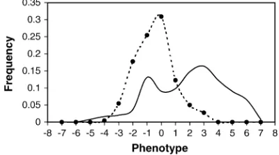
there the active alleles were different (allele heteroge-neity). The recombination fractions surrounding the simulated QTL were the following: 0.5 and 0.5 for QTL at marker 4; 0.02 and 0.2 for QTL at marker 16; and 0.1 and 0.1 for QTL at marker 30. Individual observations of two groups were then combined (464 individuals alto-gether) and a group status of each individual was ‘‘forgotten’’ in the data analysis stage. In this combined data set, the heritability attributable to each QTL at markers 4, 16, and 30 was 0.37, 0.12, and 0.05, respec-tively. This corresponds to the overall heritability of 0.55. Even if heritability in this data set may appear to be unrealistically high, the analysis presented here argu-ably corresponds to the analysis of a larger sample and smaller heritability. The simulated phenotypic distribu-tions of the two groups are shown in Figure 2. Note that these two distributions overlap reasonably well and that the same range of values is covered in both distributions. We refer to this combined data set later in the article as a complete data set.
Analyses: We sequentially increased the amount of random missingness in the genotype data. We consid-ered the complete data set and four other data sets, where 5, 10, 15, or 20% of the marker genotypes of the original complete set were coded as missing. The missingness was introduced in a nested manner so that all genotypes that were missing in the 5% data set were also missing in the 10, 15, and 20% data sets and so on. All five marker data sets (with identical phenotypes) were analyzed with the proposed method. For compar-ison, a single group analysis was also performed (which is equivalent to constraining all individuals to belong to one group only) for the data set with 5% missing values. Note that the single-group analysis closely corresponds to the methods of Kilpikariand Sillanpa¨ a¨(2003) and
Sillanpa¨ a¨ and Bhattacharjee (2005) (with
marker-independence prior), whose performances are roughly comparable to the frequentist multiple regression approaches (see the above articles for details).
The estimation of the model parameters was performed in WinBUGS 1.3 (Gilkset al.1994; Spiegelhalteret al. Figure2.—The phenotypic distributions of the two groups
drawn as frequency polygons (solid line, group 1; dotted line, group 2). The phenotypic ‘‘classes’’ (the central points indi-cated with the circles) are shown on the x-axis and corre-sponding frequencies on they-axis.
TABLE 1
The simulated values of overall mean, trait-associated markers, and additive values of their influential
alleles in the two etiology groups
Group Overall mean Marker Allele Additive value
1 2.3 4 4 3.2
16 1 2.0
2 2.3 16 3 1.2
1999) using a Pentium 4, 2.8 GHz. We used random initial values in the analyses. In all analyses, we ran two Markov chain Monte Carlo (MCMC) chains of length 25,000. The first 5000 ‘‘burn-in’’ iterations were dis-carded from each chain, which resulted in 40,000 pooled MCMC samples in total. (In analysis of the data set with 10% missing values we utilized only samples from a single chain due to reasons explained in
results.) We stored all the MCMC samples (‘‘no
thinning’’), because of a sufficient storage capacity and a low autocorrelation in the samples. Two MCMC chains were run in parallel, which took40 hr for the complete data and up to 60 hr for the 20% missing data. However, the same number of iterations for a single-group analysis took only8 hr (with 5% missing data). The conver-gence assessment was performed by visually monitoring chains for several different parameters.
SIMULATION RESULTS
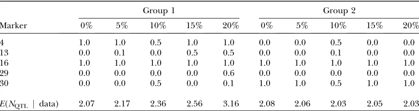
In Table 2, one can see the estimated posterior probabilities for different markers to be associated on the phenotype (i.e., QTL probabilities) at a group level and the posterior expectation (over markers) for the number of QTL in given groups. Table 2 illustrates the effect of cumulative missingness on these probabilities. In the complete data and the data set with 5% missing values, only the correct QTL positions for the two groups (markers 4, 16, and 30) are supported with QTL probability 1 and there is very little support for other positions. For comparison, the single-group analysis in the data set with 5% missing values (not shown in Table 2) resulted in nonzero QTL probabili-ties for markers 4, 16, 20, and 30 with values 1.0, 0.4, 0.1, and 0.5, respectively. With increasing missingness in Table 2, also spurious QTL positions (markers 13 and 29) gathered more support (with QTL probability
#0.6). The analysis of the data set with 10% missing values showed us that we cannot clearly identify the two
different genetic mechanisms in this case (if we utilize samples from both chains).
Labeling problem:A well-known problem in this kind of population assignment method is the weak identifi-ability of the labels of the two groups (see Pritchard
et al. 2000b; Stephens 2000). This means that
some-times the group configurations obtained in one analysis end up as their mirror image in another analysis just because of the symmetry in the likelihood of the pa-rameters (Figure 3). Following the standard practice of sophisticated population assignment methods in ge-netics, like those of Pritchard et al.(2000b), there is
nothing in the model, except the initial values of the MCMC sampler, to attach individuals of group one to the group with index one. The suggested solution for this problem is to impose some order constraints on one of the parameters such as constraining the groups to have increasing means or increasing proportions of individuals in the groups (Richardson and Green
1997; Stephens2000). However, R. M. Neal’s comment
in Kass et al. (1998) was strongly against using such
constraints, because they can do serious harm to the convergence. Here such constraints presumably do not provide good identifiability for the groups and compli-cate interpretation, because the information with re-spect to the groups at some loci seems to be too weak on the basis of our experiences with the secondary analysis (see conditional analyses below). In unconstrained models such as the one here, it can actually be pref-erable that the MCMC sampler is mixing poorly with respect to symmetry of the two groups (i.e., label switch-ing does not occur), because it simplifies interpretation of the results (see Pritchardet al. 2000b). Note that
Celeuxet al.(2000) have suggested a tempering scheme
for assignment models to improve the mixing properties of the sampler. As is typical in population assignment methods (see Pritchardet al.2000b), the label
switch-ing did not occur within any sswitch-ingle MCMC chain in our analyses. Such a behavior was found here only between
TABLE 2
Group-specific QTL probabilities
Group 1 Group 2
Marker 0% 5% 10% 15% 20% 0% 5% 10% 15% 20%
4 1.0 1.0 0.5 1.0 1.0 0.0 0.0 0.5 0.0 0.0
13 0.0 0.1 0.0 0.5 0.5 0.0 0.0 0.1 0.0 0.0
16 1.0 1.0 1.0 1.0 1.0 1.0 1.0 1.0 1.0 1.0
29 0.0 0.0 0.0 0.0 0.6 0.0 0.0 0.0 0.0 0.0
30 0.0 0.0 0.5 0.0 0.1 1.0 1.0 0.5 1.0 1.0
E(NQTL j data) 2.07 2.17 2.36 2.56 3.16 2.08 2.06 2.03 2.05 2.03
two separate MCMC chains with the data set with 10% missing values.
Conditional analyses:With real data, one may not be able to decide if the estimated genetic architecture is unclear (not unique) because of the label switching or because of the complexity of the underlying genetic architecture. Even though it was known in our simula-tion study that the label switching was responsible, we still performed the additional analyses with the data set having 10% missing values to illustrate one possible approach. Three additional analyses were performed so that a locus-indicator pair (corresponding to two groups) at a single locus of the three markers (4, 16, and 30) was kept fixed throughout the MCMC estimation process. These three conditional analyses are ‘‘short cuts’’ for exhaustive enumeration of analyses where all possible combinations of the gene actions over these three loci are fixed one at a time. However, we can still gain some further information about the genetic architecture this way. Two parallel chains were run with 10,000 iterations in each (the first 2500 iterations from both were discarded, as burn in). This resulted in 15,000 effective MCMC samples in total.
In the first conditional analysis, where two group-specific locus indicators of marker 4 were
simulta-neously fixed to values ofI4,1¼1 andI4,2¼0, the
anal-ysis was able to reconstruct the true underlying genetic architecture extremely well, having well-structured QTL probabilities of the two groups at markers 16 (1.0, 1.0) and 30 (0.1, 1.0) and a negligible support for marker 13 (0.1, 0.0), respectively. In the second analysis, where two indicators of marker 16 were fixed to values ofI16,1¼1
and I16,2 ¼ 0, several nonzero QTL probabilities
appeared at new (incorrect) marker positions in partic-ular for group 2, indicating that the locus indicatorI16,2
should not be zero. This was further supported also by the QTL probabilities in group 1 for markers 4 and 30, which were 0.5 and 0.5, respectively. In the third analysis, where the two indicators of marker 30 were fixed to values ofI30,1¼1 andI30,2¼0, the problem of
label switching occurred again even after the constraint so that two MCMC samples were mirror images of each other (excluding the fixed locus 30). This behavior might be an indication of the weak genetic effect of marker 30 (cf. the simulated effect sizes of Table 1). However, one of the two MCMC chains converged to the same structure supported by the first conditional anal-ysis (of marker 4), which also happened to be the true underlying structure.
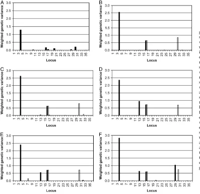
Summarizing QTL effects: Because a random
vari-ance model was used for QTL effects, it is natural to look first at the posterior estimates of genetic variances and then at the sizes of the individual effects. As expected, the estimated genetic variances (their posterior means) at positions with low QTL probabilities are very close to their prior mean 1 (the results not shown). This is because in our model the data do not influence the genetic variance estimate in the MCMC rounds where the corresponding locus indicator value is zero. Due to (i) assuminga prioriindependence of the indicators and genetic effects (cf.Kuoand Mallick1998), (ii)
assum-ing only a sassum-ingle genetic variance parameter for each marker, and (iii) assuming a nonzero prior mean for the genetic variance, we summarize our results in two groups in the form of weighted genetic variances (Ilj3
sl2) in Figure 4. The weighted genetic variance is actually
the model-averaged estimate of the genetic variance (averaged over all models with the effect set to zero in models where the marker for a given group was not selected) (Sillanpa¨ a¨ and Bhattacharjee 2005). See
the discussion for the motivation for points i and
ii above. (Because of point iii above, we expected to obtain better mixing properties for the sampler and avoid confounding between locus indicators and genetic effects, leading to better estimates of QTL probabilities.) The estimates of Figure 4 are based on the additional analysis with two parallel MCMC chains (both of length 1500 and no burn in), where the last states of param-eter values (of earlier 25,000 MCMC rounds) were used as starting values. (In practice this can be seen also as discarding 25,000 MCMC samples as burn in from each chain.) For a comparison, the weighted genetic
Figure3.—Illustration of how markers selected to be active
variances from the single-group analysis (in the data set with 5% missing values) are also shown (Figure 4A).
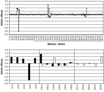
Dissecting allelic heterogeneity: The posterior esti-mates of locus-specific allelic effects at two groups for complete data are shown in Figure 5. In the top, one can see that only three simulated QTL seem to have non-negligible estimated allelic effects, which are shown in more detail below (Figure 5, bottom). Since we did not impose any constraints for the coefficients, one should interpret the graphs with respect to that. (One can impose constraints afterward by setting the first co-efficient to zero and looking at differences (contrasts) of estimated coefficients at each locus.) If the constraints are imposed afterward, then only four true alleles seem to have nonnegligible effects (allele 4 at marker 4, alleles 1 and 3 at marker 16, and allele 5 at marker 30), which closely correspond to the simulated values of Table 1. In Figure 5, bottom, we observe that marker 16 is the only one showing evidence of allelic heterogeneity and the evidence is with respect to the correct alleles (1 and 3).
Concordance in assignments: To illustrate how well the individual assignments can be identified from five different data sets, Table 3 presents the numbers of
correctly and incorrectly classified individuals in each group. The estimated group for each individual is based on the posterior mean estimate of the group assign-ment. The posterior mean estimated proportion of individuals belonging to the smaller of the two groups is also shown (true value is 0.47). Note that the pro-portion of incorrectly classified individuals is slowly increasing with the amount of missing data, but the ‘‘prop of inds’’, which equalsp(k2 j y,mobs,s), does not
seem to do so. We would have expected to see this behavior in the case that the prior value for the proportion of individuals belonging to the one of the two groups was 0.5, corresponding to a uniform prior on the group assignment variable (Ei).
Estimated overall means:Table 4 shows how well the group-specific overall mean parameters (true values are 2.3 and2.3) were estimated from five different data sets using the proposed approach and the single-group analysis (with the constraint that all individuals belong to group 1). Although only the posterior means are shown, they can still illustrate how estimates have been shrunk toward zero by increasing the amount of missing values or assuming only a single group. Note that the
Figure4.—The weighted
single-group analysis was performed only for the data set with 5% missing observations.
REAL DATA ANALYSIS
Cystic fibrosis data, model, and analysis: As in Sillanpa¨ a¨ and Bhattacharjee(2005), we selected a
well-known cystic fibrosis (CF) data set (Kerem et al.
1989), with binary phenotype and 23 biallelic markers
collected from 93 individuals. The markers in this data set span the 1.7-Mb region surrounding the cystic fibrosis transmembrane regulator (CFTR) gene on chromosomal segment 7q31. The data set contains the haplotype information (without individual identities) and the physical distances (Keremet al.1989; Morris
et al.2000), and there is some degree of missing alleles. As earlier (Sillanpa¨ a¨ and Bhattacharjee 2005), we
use a marker-dependence prior (withs¼ 1
23) to utilize
physical distances and the model where each individual contributed two independent observations (phenotype and one allele in each locus) to the analysis. The prior for the overall smoothing parameter is Gamma(1, 0.01)
Figure5.—QTL allelic effects.
Locus-specific point estimates (posterior mean) of allelic effects in two groups for complete data. The effects are shown for all the markers (top) and for the markers having nonnegligible ef-fects on the phenotype (bottom). The marker and allele numbers are shown on the x-axis and allelic effects on the y-axis. In the top, the allelic effects are presented as a curve (frequency poly-gon) in two groups (solid line, group 1; shaded line, group 2). Vertical lines in the bottom indicate change of marker.
n
, group 1;h, group 2.TABLE 3
Cross-tabulations of posterior mean classifications with respect to their original groups
(Original group, estimated group)
Data (%) (1, 1) (1, 2) (2, 1) (2, 2) Prop of inds
0 202 42 51 169 0.45
5 198 46 50 171 0.46
10 195 49 49 171 0.47
15 193 51 54 166 0.47
20 188 56 56 164 0.47
Different percentages (0, 5, 10, 15, and 20%) indicate the different data sets with corresponding percentage of missing values. ‘‘Prop of inds’’ indicates the posterior mean estimated proportion of individuals that are members in the smaller of the two groups (which happened to be group 2 here) esti-mated from sampled values for hyperparameterk2. For all data sets, the estimates are presented on the basis of the group labels giving the best fit. Note that only a single MCMC chain was utilized in the 10% data set.
TABLE 4
The posterior mean estimates of overall mean in two-group and single-group analyses
Group
Data (%) 1 2 Single-group analysis
0 1.66 1.23
5 1.95 1.16 0.43
10 1.40 1.07
15 1.53 0.86
20 1.39 0.82
with prior mean at 100. A difference from our earlier analysis (Sillanpa¨ a¨ and Bhattacharjee 2005) is that
here the haplotype information is utilized—each haplo-type is classified into one of the two etiology groups. By using such an independent-observation idea (Sasieni
1997), sample size is doubled, only a single allelic coefficient is fitted in each selected locus for each observation, and estimated effects are approximately double in size. Note that here we are effectively carrying out a heterogeneity analysis for the alleles with respect to their parental origins. Note also that, unlike Sillanpa¨ a¨
and Bhattacharjee(2005), we use a random variance
model for genetic effects and the prior for missing values where each allele is considered to be a priori equally probable at each marker locus. Because of the binary phenotype, we do not have prior for precision parameter. Otherwise, we use the same priors as in the simulated data analyses.
The parameter estimation was done in WinBUGS 1.3 (Gilkset al.1994; Spiegelhalteret al.1999), using a
Pentium 4, 3.40 GHz. Two parallel MCMC chains each of length 7800 were run with random initial values that took29 hr. Because of 300 burn-in iterations per chain and no thinning, this resulted in 15,000 pooled MCMC samples in total. No evidence of label switching or con-vergence problems was detected by our visual inspec-tion of MCMC chains for several different parameters.
Results of CF data: In Figure 6, we present values of weighted genetic variances estimated for two etiology groups. Only locus 2 shows a highly elevated value in group 1 whereas we can see two elevated peaks at positions 10 and 17 in group 2. The estimated propor-tions of haplotypes classified into two groups, respec-tively, were 0.2 and 0.8, and individual assignment probabilities were found to be surprisingly high, making unambiguous membership identification possible for most of the haplotypes. The two positions (10 and 17) as well as their weighted genetic variance peaks in group 2 are very similar to what was found in the single-group
analysis of Sillanpa¨ a¨ and Bhattacharjee (2005).
(Note that only QTL probabilities were shown in Sillanpa¨ a¨ and Bhattacharjee 2005). However, one
can see how the peak of position 2 in group 1 has grown much higher in the two-group analysis, changing the overall conclusion for that position. Note that Lazzeroni
(1998) also found a notably high peak at position 2. Further exploration of the haplotype data was per-formed for a subset of haplotypes that showed very high assignment probability (.0.75) to one of the two groups. This led us to 169 classified haplotypes of a total of 186. This exercise revealed that although locus 2 was identified as an influential position in group 1, allele frequencies at this marker were not visibly different for two groups when compared to frequencies calculated from the whole data set. Surprisingly, it was locus 17 that showed a remarkable allele frequency difference between the two etiology groups (suggesting that position 17 could actually be a stratifying factor). Moreover, a large proportion of haplotypes in group 1 were observed to have allele 2 at locus 17 co-occurring with allele 1 at locus 2 (suggesting the existence of epistatic interaction between loci 17 and 2). At locus 10, we observed a minor increase of frequency of allele 2 in group 1 and of allele 1 in group 2 but the difference was much milder than that at locus 17.
Finally, we wanted to check whether the estimated stratification of haplotypes (in the two groups) is connected to any of the known stratifiers—mutation subsets presented in Table 3 of Keremet al.(1989). The
membering CF haplotypes are identified according to whether they carry the DF508 or other mutations and
are additionally within each of two mutation groups— those with pancreatic insufficiency (PI) or pancreatic sufficiency (PS). The inspections were done by moni-toring the posterior estimated number of patient hap-lotypes that were classified to group 1 and that also had the non-DF508mutation, posterior estimated
num-ber of haplotypes classified to group 1, and so on. (This monitoring was based on a separate MCMC run.) On the basis of the posterior estimates we observed that the frequency of CF haplotypes containing the non-DF508
mutation showed clear enrichment in group 1 (the smaller group with locus 2 as the main QTL) while the frequency of haplotypes carrying the DF508 mutation
showed no difference. From this we may conclude/ suggest that if there is epistatic interaction between loci 17 and 2, it is likely to occur in haplotypes with the
non-DF508mutation on the CF chromosome.
Type 2 diabetes mellitus and model: These data
were first published in a positional cloning study of Horikawaet al.(2000) and a subset of data has been
reanalyzed by Zo¨ llnerand Pritchard(2005). We use
the same subset of data as Zo¨ llner and Pritchard
(2005), which have a binary phenotype (108 cases and 112 controls) and 85 SNP markers (with physical dis-tances) spanning the 876-kb area in the NIDDM1 region
Figure 6.—Locus-specific point estimates (posterior
on chromosome 2. However, there is one important difference between our approaches: before the actual association analysis, Zo¨ llner and Pritchard (2005)
completed missing alleles with their most likely values and estimated haplotypes using the PHASE program whereas we use raw genotype data with missing values directly in our analysis. We use the model where every individual contributes a single observation (phenotype and two alleles at each locus) to the analysis. We use a random variance model for genetic effects and the prior for missing values where each allele is considered to bea prioriequally probable at each marker locus.
The parameters were estimated using two different values of shrinkage parameter:s¼ 1
85(shrinkage) and
s¼1
2(no shrinkage) in WinBUGS 1.3 (Gilkset al.1994;
Spiegelhalter et al. 1999), using a Pentium 4, 3.40
GHz. Two parallel MCMC chains each of length 5500 and 3750 (no shrinkage) were run with random initial values, which took25 sec per iteration (with two par-allel chains). By having burn in of 500 and 2500 (no shrinkage) iterations per chain and no thinning, the estimations were based on 10,000 and 2500 (no shrink-age) pooled MCMC samples in total. Again, no prob-lems in label switching or convergence were detected.
Results of diabetes data:The analysis with shrinkage parameters¼ 1
85and marker-independence prior (no
distances) ended up with a clear signal at 269 kb in group 1. The estimated proportion of individuals therein is 0.73. To see if any additional positions can be found by relaxing the stringency on the shrinkage pa-rameter, another analysis was executed with the shrink-age paramameters¼1
2. (Note that half of the genes are
assumed to be associateda prioriunder this setting.) As presented in Figure 7, two additional positions at 160 and 161 kb were identified to be active in both groups. One can see that there are weak signals also at 269 and 400 kb in group 2. The estimated proportion of individuals in group 1 is 0.62. The estimated position of disease mutation in Zo¨ llnerand Pritchard(2005)
is at 131 kb and the three SNPs that make up the hap-lotype at CAPN-10 (Horikawaet al.2000) are located
at 121, 124, and 134 kb. Overall, our estimates are
somewhat to the right of their estimates. Zo¨ llnerand
Pritchard (2005) emphasized that the presence of
other genes cannot be excluded because their signal was only modestly significant.
Finally, the complementary analysis was executed with the model using the marker-dependence prior (with distances). This analysis seemed to confirm the loca-tions that were already found in the marker-indepen-dence prior analysis (details and results not shown).
DISCUSSION
Presence of genetic heterogeneity: Generally the
most efficient ways to reduce genetic heterogeneity of the trait in the sample are applicable only in the de-sign stage of the study. Examples of those practices are: (1) careful phenotype definition (Leboyeret al.1998;
Sillanpa¨ a¨2002) based on expression profiling (Kraft
and Horvath 2003) or proteomics data (Semmes
2004), (2) careful choice of study population (Wright
et al. 1999; Peltonen 2000; Shifman and Darvasi
2001), and (3) careful sample collection such as utilization of the known history of the population isolate in ascertainment (Heathet al.2001). In this article, we
emphasize that we have considered the case where such preventative actions cannot be applied or they have not been sufficient in homogenizing the sample. Moreover, one can consider using this method as a test of presence of genetic heterogeneity or as a primary analysis when there is already some prior evidence or a hint about genetic heterogeneity obtained by statistical or biolog-ical means: (1) association testing cannot find a signal, (2) findings from earlier studies cannot be replicated or are contradictory, (3) the population consists of indi-viduals from several ethnic backgrounds, or (4) there is multimodality of the phenotype distribution. Note that one can also use this approach to argue if (self-reported or estimated) ethnic background can be used as a known factor giving specification for the etiological groups.
The presented method: We have presented a new
method for studying multilocus association between multiple marker loci and a quantitative or binary trait in
Figure 7.—The point estimates (posterior
mean) of weighted genetic variances in two groups for the diabetes data with the model having marker-independence prior and with-out shrinkage (s¼1
the presence of genetic heterogeneity. The method can handle multiallelic marker loci with some degree of missing genotypes. On the basis of tested examples, the amount of missing data should not be too large (roughly not more than 15%). We expect this to be even more critical in binary traits, where phenotype carries less information. This method can be implemented with WinBUGS (Gilks et al. 1994; Spiegelhalter et al.
1999), which automatically calculates data-specific tun-ing parameters needed in a Metropolis–Hasttun-ings ran-dom walk (Chiband Greenberg1995). Additionally, by
assuminga priori independence of the indicators and genetic effects (cf. Kuo and Mallick 1998), we can
avoid the existence of other difficult tuning parameters like those needed in stochastic search variable selection (Georgeand McCulloch 1993; Yiet al.2003a). The
method allows for use of external covariates such as age, sex, environmental risk factors, gene-expression mea-surements (see Hoti and Sillanpa¨ a¨ 2006), and
dom-inance in the genetic model. However, we do not claim that this approach is robust for bias of population stratification although logistic regression should be a relatively safe approach in the case of binary phenotype (see Setakis et al. 2006). If marker data have been
collected from some specific chromosomal interval, one can control for the problem of population stratification (and other confounders) by using the marker-depen-dence prior of locus indicators to incorporate physical or genetic map distances, similarly as in Sillanpa¨ a¨and
Bhattacharjee(2005). In other cases, we propose the
use of self-identified ethnicity or structured association to handle the problem of population stratification (Pritchard et al. 2000a,b; Sillanpa¨ a¨ et al. 2001;
Coranderet al.2003, 2004; Hoggartet al.2003). Note
that a self-reported population identity given by a per-son (or identity estimated by STRUCTURE or BAPS soft-ware) is a putative classification covariate that could be handled as an extra ‘‘marker locus’’ in the presented method.
Stratifying factor and label switching: As an output, our method provides estimates for group-specific ge-netic models (QTL) and individual assignments to the groups. In the estimated groups and their QTL, one cannot distinguish if the group-specific locus was identified because of genetic heterogeneity or because of interaction between the locus and some unmeasured (or unused) environmental covariate (see Thorton
-Wellset al.2004). One can, however, check this
after-ward with respect to existing (but unused) covariates that are available, but generally this is an intractable problem. One should keep this in mind when conclu-sions are drawn from the analysis. Like some other sophisticated population assignment methods in genet-ics, our method is likely to suffer from the problem of label switching between different MCMC chains (Pritchardet al.2000b; Stephens2000). We did not
encounter label switching within any single MCMC
chain in our test examples. This (no label switching) simplifies interpretation of the results (groups have labels) but it is also an indication of poor mixing of the MCMC sampler, which one should be aware of and monitor carefully. When label switching occurs across chains (but not within a chain), one should calculate posterior estimates on the basis of samples from a single long MCMC chain instead of pooling samples together from several shorter MCMC runs (even if monitoring the convergence and detection of this problem is based on running several MCMC chains). Moreover, one can also apply the conditional analysis for unclear cases to dissect the underlying structure further, as was illus-trated inresults. As a conclusion, we emphasize that
even if label switching within a single MCMC chain happens, one can still obtain valuable information about the existence of genetic heterogeneity from this analysis when compared to the results of single-group analysis. That is, if the same set of loci is supported by both groups and this set differs from single-group analysis, one can conclude that it is likely that there is genetic heterogeneity and label switching.
Computation:As was illustrated in the examples, our approach requires a substantial amount of computation time. Therefore, the current WinBUGS implementa-tion may not directly scale to extremely large sizes of data (with thousands of individuals) or large marker sets (with several hundreds of markers). Thus, for large-scale data sets: (1) the size of the problem can be reduced by focusing on a subgroup of genes (e.g., on the basis of known pathways, specific genomic regions, or preliminary screening or dimension-reduction techni-ques), and/or (2) one can pursue faster implementa-tion of the method by using C-language, and (3) one can concentrate on the estimating mode (maximuma posteriori, MAP) of the posterior distribution only. However, an extra level of difficulty in methods 2 and 3 above (avoided here by WinBUGS) is to find a good updating scheme for the MCMC sampler. Finally, it is also possible in a Bayesian framework to first divide individuals in the data into the smaller data sets and analyze them separately. Because the posterior distribu-tion (results) from one analysis can always be taken as a prior distribution to the next analysis, it is possible to combine separate analyses together afterward and to produce still a meaningful summary. However, we do not recommend such a ‘‘split and combine’’ approach here, because of the weak identifiability of the groups and potential labeling problems.
Differences between methods:Because the proposed method can be seen as an extension of the earlier work (Sillanpa¨ a¨et al.2001; Kilpikariand Sillanpa¨ a¨2003;
Sillanpa¨ a¨ and Bhattacharjee2005) we briefly
com-ment on the differences between these methods:
1. Population assignment: Sillanpa¨ a¨et al.(2001) also
set of neutral markers were included as an extra in-formation source (which is useful for correcting pop-ulation stratification but not neccessarily for genetic heterogeneity). Kilpikari and Sillanpa¨ a¨ (2003)
and Sillanpa¨ a¨ and Bhattacharjee(2005)
consid-ered only a case of single-population analysis. 2. Locus indicators and a random variance model:
Sillanpa¨ a¨et al.(2001) and Kilpikariand Sillanpa¨ a¨
(2003) employed the reversible-jump MCMC for candidate (QTL) selection and a fixed-variance model (fixed-effect model) for QTL effects, whereas Sillanpa¨ a¨and Bhattacharjee(2005) as well as the
approach here utilized locus-indicator variables for genetic model selection and a random-variance model (variance-component model) for QTL effects. How-ever, the reversible-jump MCMCs in these approaches were implemented in a way that resembles locus-indicator models (see Kilpikariand Sillanpa¨ a¨2003).
3. Two groups share a common variance: The special property of the model presented here is that the group-specific effects (at each locus) are assumed to be exchangeable; that is, they share a distribution with the common variance component. In the case that the QTL (marker) is active in both groups, all observations contribute to the estimation of the cor-responding genetic variance. This means that in the homogeneous case, where the same sets of QTL are simultaneously present in two groups, the approach can maintain the power comparable to that of the single-group analysis. Sillanpa¨ a¨et al.(2001)
consid-ered an individual parameter set for each group, which is not optimal in the homogeneous case.
Number of groups:In the analysis, we have assumed that the number of etiology groups is two and that the residual variance (precision) parameter is common for both groups. If the number of true underlying groups is one this is not a problem (see above paragraph). However, the method can also be generalized for a larger (more than two) number of groups if there is somea prioriinformation about the groups and identifi-ability is not a problem. Nevertheless, the number of distinct modes of the phenotype distribution should not be directly used as a number of groups (cf.Figure 2). For a large number of groups, it may still be best to assume only two groups but use group-specific residual varian-ces. This kind of model would follow the spirit of an admixture model, where one tries to fit a common disease model only for the homogeneous part of the data and puts the rest of the data into a ‘‘junk group,’’ which can include phenocopies and all kinds of indi-viduals from multiple genetic backgrounds.
Epistasis:We share the view (Sillanpa¨ a¨2002; Moore
2003; Sillanpa¨ a¨ and Auranen2004; Thorton-Wells
et al.2004) that the dissection of complex traits requires novel methods that are capable of handling both the genetic heterogeneity and complex genetic
architec-ture. The current approach does use multilocus estima-tion and can account for genetic heterogeneity but does not explicitly model epistatic interactions. Although it may be easy to include known pairs of epistatic markers in the model (e.g., based on database information on known pathways; see Thomas 2005), detection of
epistasis is generally a difficult task that requires a suitable combination of the following: specific designs, large data sets, appropriate statistical modeling, and high computing power. In spite of these difficulties, an extension of the presented approach that includes epistasis and utilizes the modern ideas of stochastic partitioning where genotypes from multiple loci are stochastically pooled into a smaller number of classes (see Moore 2003; Sillanpa¨ a¨ and Auranen 2004)
would be worth of considering in the future. For current Bayesian interaction approaches, see Conti et al.
(2003), Yiand Xu(2002), Yiet al.(2003b, 2005), Narita
and Sasaki(2004), and Zhangand Xu(2005).
The model specification code (written in WinBUGS) is freely available for research purposes at http:// www.rni.helsinki.fi/mjs/.
We are grateful to Nancy Cox, Jonathan Pritchard, and Sebastian Zo¨llner for their help with the diabetes data; to Andrew Morris, Kung-Yee Liang, and Yen-Feng Chiu for their help with the CF data; and to Andrew Thomas, Duncan C. Thomas, and two anonymous referees for their constructive comments on the manuscript. This work was supported by research grant no. 202324 from the Academy of Finland.
LITERATURE CITED
Balding, D., A. D. Carothers, Y. L. Marchini, L. R. Cardon, A. Vetta
et al., 2002 Discussion on the meeting on statistical modelling and analysis of genetic data. J. R. Stat. Soc. B64:737–775. Broman, K. W, and T. P. Speed, 2002 A model selection approach
for identification of quantitative trait loci in experimental crosses. J. R. Stat. Soc. B64:641–656.
Bull, S. B., L. Mirea, L. Briollaisand A. G. Logan, 2003 Het-erogeneity in IBD allele sharing among covariate-defined sub-groups: issues and findings for affected relatives. Hum. Hered.
56:94–106.
Burchard, E. G., Z. Elad, N. Coyle, S. L. Gomez, H. Tanget al., 2003 The importance of race and ethnic background in bio-medical research and clinical practice. N. Engl. J. Med. 348:
1170–1175.
Cardon, L. R., and L. J. Palmer, 2003 Population stratification and spurious allelic association. Lancet361:598–604.
Celeux, G., M. Hurnand C. P. Robert, 2000 Computational and inferential difficulties with mixture posterior distributions. J. Am. Stat. Assoc.95:957–970.
Chib, S., and E. Greenberg, 1995 Understanding the Metropolis-Hastings algorithm. Am. Stat.49:327–335.
Clayton, D., 2001 Population association, pp. 519–540 inHandbook
of Statistical Genetics, edited by D. J. Balding, M. Bishopand C. Cannings. Wiley, Chichester, UK.
Conti, D. V., and J. S. Witte, 2003 Hierarchical modeling of linkage disequilibrium: genetic structure and spatial relations. Am. J. Hum. Genet.72:351–363.
Conti, D. V., V. Cortessis, J. Molitorand D. C. Thomas, 2003 Bayesian modeling of complex metabolic pathways. Hum. Hered.56:83–93.
Cooper, R. S., J. S. Kaufman and R. Ward, 2003 Race and ge-nomics. N. Engl. J. Med.348:1166–1170.
Corander, J., P. Waldmannand M. J. Sillanpa¨ a¨, 2003 Bayesian analysis of genetic differentiation between populations. Genetics
Corander, J., P. Waldmann, P. Marttinenand M. J. Sillanpa¨ a¨, 2004 BAPS 2: enhanced possibilities for the analysis of the ge-netic population structure. Bioinformatics20:2363–2369. Devlin, B., and K. Roeder, 1999 Genomic control for association
studies. Biometrics55:997–1004.
Devlin, B., K. Roederand L. Wasserman, 2003 Analysis of multi-locus models of association. Genet. Epidemiol.25:36–47. Durrant, C., K. T. Zondervan, L. R. Cardon, S. Hunt, P. Deloukas
et al., 2004 Linkage disequilibrium mapping via cladistic analy-sis of single-nucleotide polymorphism haplotypes. Am. J. Hum. Genet.75:35–43.
Ekstrom, C. T., and P. Dalgaard, 2003 Linkage analysis of quanti-tative trait loci in the presence of heterogeneity. Hum. Hered.55:
16–26.
Epstein, M. P., C. D. Veal, R. C. Trembath, J. N. W. N. Barker, C. Li
et al., 2005 Genetic association analysis using data from triads and unrelated subjects. Am. J. Hum. Genet.76:592–608. Ewens, W. J., and R. S. Spielman, 1995 The
transmission/disequi-librium test: history, subdivision, and admixture. Am. J. Hum. Genet.57:445–464.
Flint, J., and R. Mott, 2001 Finding the molecular basis of quan-titative traits: successes and pitfalls. Nat. Rev. Genet.2:437–445. Foster, M. W., and R. R. Sharp, 2004 Beyond race: towards a whole-genome perspective on human populations and genetic varia-tion. Nat. Rev. Genet.5:790–796.
Gasbarra, D., M. J. Sillanpa¨ a¨and E. Arjas, 2005 Backward simu-lation of ancestors of sampled individuals. Theor. Popul. Biol.67:
75–83.
George, E. I., and R. E. McCulloch, 1993 Variable selection via Gibbs sampling. J. Am. Stat. Assoc.88:881–889.
Gilks, W. R., A. Thomasand D. J. Spiegelhalter, 1994 A language and program for complex Bayesian modeling. Statistician 43:
169–178.
Grigull, J., R. Alexandrovaand A. D. Paterson, 2001 Clustering of pedigrees using marker allele frequencies: impact on linkage analysis.Genet. Epidemiol.21(Suppl. 1): S61–S66.
Hauser, E. R., R. M. Watanabe, W. L. Duren, M. P. Bass, C. D. Langefeldet al., 2004 Ordered subset analysis in genetic link-age mapping of complex traits. Genet. Epidemiol.27:53–63. Heath, S., R. Robledo, W. Beggs, G. Feola, C. Parodoet al., 2001
A novel approach to search for identity by descent in small sam-ples of patients and controls from the same Mendelian breeding unit: a pilot study on Myopia. Hum. Hered.52:183–190. Hinds, D. A., R. P. Stokowski, N. Patil, K. Konvicka, D. Kershenobich
et al., 2004 Matching strategies for genetic association studies in structured populations. Am. J. Hum. Genet.74:317–325. Hodge, S. E., V. J. Vielandand D. A. Greenberg, 2002 HLODs
re-main powerful tools for detection of linkage in the presence of genetic heterogeneity. Am. J. Hum. Genet.70:556–558. Hoggart, C. J., E. J. Parra, M. D. Shriver, C. Bonilla, R. A. Kittles
et al., 2003 Control of confounding in genetic associations in stratified populations. Am. J. Hum. Genet.72:1492–1504. Horikawa, Y., N. Oda, N. Cox, X. Li, M. Orho-Melanderet al.,
2000 Genetic variation in the gene encoding calpain-10 is asso-ciated with type 2 diabetes mellitus. Nat. Genet.26:163–175. Hoti, F., and M. J. Sillanpa¨ a¨, 2006 Bayesian mapping of genotype
3expression interactions in quantitative and qualitative traits. Heredity97:4–18.
Hoti, F., A. Tuulio-Hendriksson, J. Haukka, T. Partonen, L. Holmstro¨ met al., 2004 Family-based clusters of cognitive test performance in familial schizophrenia. BMC Psychiatry4:20. International HapMap Consortium, 2003 The international
HapMap project. Nature426:789–796.
InternationalHapMapConsortium, 2005 A haplotype map of the human genome. Nature437:1299–1320.
Kass, R. E., B. P. Carlin, A. Gelmanand R. M. Neal, 1998 Markov chain Monte Carlo in practice: a roundtable discussion. Am. Stat.
52:93–100.
Kazeem, G. R., and M. Farrall, 2005 Integrating case-control and TDT studies. Ann. Hum. Genet.69:329–335.
Kerem, B.-S., J. M. Rommens, J. A. Buchanan, D. Markiewicz, T. K. Coxet al., 1989 Identification of the cystic fibrosis gene: genetic analysis. Science245:1073–1080.
Kilpikari, R., and M. J. Sillanpa¨ a¨, 2003 Bayesian analysis of multi-locus association in quantitative and qualitative traits. Genet. Ep-idemiol.25:122–135.
Knapp, M., and T. Becker, 2003 Family-based association analysis with tightly linked markers. Hum. Hered.56:2–9.
Kraft, P., and S. Horvath, 2003 The genetics of gene expression and gene mapping. Trends Biotechnol.21:377–378.
Kuo, L., and B. Mallick, 1998 Variable selection for regression models. Sankhya Ser. B60:65–81.
Lander, E. S., and N. J. Schork, 1994 Genetic dissection of com-plex traits. Science265:2037–2048.
Lazzeroni, L. C., 1998 Linkage disequilibrium and gene mapping: an empirical least-squares approach. Am. J. Hum. Genet. 62:
159–170.
Leal, S. M., 1997 Tests for detecting linkage and linkage heteroge-neity, pp. 97–112 inGenetic Mapping of Disease Genes, edited by I. H. Pawlowitzki, J. H. Edwardsand E. A. Thompson.. Academic Press, San Diego.
Leal, S. M., and J. Ott, 2000 Effects of stratification in the analysis of affected-sib-pair data: benefits and costs. Am. J. Hum. Genet.
66:567–575.
Leboyer, M., F. Bellivier, M. Nosten-Bertrand, R. Jouvent, P. Davidet al., 1998 Psychiatric genetics: search for phenotypes. Trends Neurosci.21:102–105.
Lin, Z., and R. B. Altman, 2004 Finding haplotype tagging SNPs by use of principal component analysis. Am. J. Hum. Genet.75:
850–861.
Lohmueller, K. E., C. L. Pearce, M. Pike, E. S. Landerand J. N. Hirchorn, 2003 Meta-analysis of genetic association studies supports a contribution of common variants to susceptibility to common diseases. Nat. Genet.33:177–182.
Longmate, J. A., 2001 Complexity and power in case-control asso-ciation studies. Am. J. Hum. Genet.68:1229–1237.
Marchini, J., L. R. Cardon, M. S. Phillips and P. Donnelly, 2004 The effects of human population structure on large ge-netic association studies. Nat. Genet.36:512–517.
Meng, Z., D. V. Zaykin, C.-F. Xu, M. Wagnerand M. G. Ehm, 2003 Selection of genetic markers for association analyses, using link-age disequilibrium and haplotypes. Am. J. Hum. Genet.73:115–130. Molitor, J., P. Marjoramand D. Thomas, 2003a Fine-scale map-ping of disease genes with multiple mutations via spatial cluster-ing techniques. Am. J. Hum. Genet.73:1368–1384.
Molitor, J., P. Marjoramand D. Thomas, 2003b Application of Bayesian spatial statistical methods to analysis of haplotypes ef-fects and gene mapping. Genet. Epidemiol.25:95–105. Moore, J. H., 2003 The ubiquitous nature of epistasis in
determin-ing susceptibility to common human diseases. Hum. Hered.56:
73–82.
Morris, A., J. C. Whittakerand D. J. Balding, 2000 Bayesian fine-scale mapping of disease loci, by hidden Markov models. Am. J. Hum. Genet.67:155–169.
Morris, A. P., J. C. Whittakerand D. J. Balding, 2002 Fine-scale mapping of disease loci via shattered coalescent modeling of ge-nealogies. Am. J. Hum. Genet.70:686–707.
Morris, A. P., J. C. Whittaker, C.-F. Xu, L. K. Hostingand D. J. Balding, 2003 Multipoint linkage-disequilibrium mapping narrows location interval and identifies mutation heterogeneity. Proc. Natl. Acad. Sci. USA100:13442–13446.
Narita, A., and Y. Sasaki, 2004 Detection of multiple QTL with ep-istatic effects under a mixed inheritance model in an outbred population. Genet. Sel. Evol.36:415–433.
Peltonen, L., 2000 Positional cloning of disease genes: advantages of genetic isolates. Hum. Hered.50:66–75.
Pritchard, J. K., M. Stephens, N. A. Rosenbergand P. Donnelly, 2000a Association mapping in structured populations. Am. J. Hum. Genet.67:170–181.
Pritchard, J. K., M. Stephensand P. Donnelly, 2000b Inference of population structure using multilocus genotype data. Genetics
155:945–959.