New Bounds on Image Denoising Using Non Local PCA Algorithm for Noise Estimation

(1)

ISSN(Online) : 2319-8753 ISSN (Print) : 2347-6710

I

nternational

J

ournal of

I

nnovative

R

esearch in

S

cience,

E

ngineering and

T

echnology

(An ISO 3297: 2007 Certified Organization)

Vol. 5, Issue 4, April 2016

New Bounds on Image Denoising Using Non

Local PCA Algorithm for Noise Estimation

N.Veni1, G.Jayandhi2

Assistant Professor, SRM University, Chennai, India1

Assistant Professor, Velammal Engineering College, Chennai, India 2

ABSTRACT: Image denoising algorithmsoften assume an additive white Gaussian noise (AWGN) process that is independent of the actual RGB values. Such approaches are not fully automatic and cannot effectively remove colour noise produced by today’s CCD digital camera. In this paper, we propose a unified framework for two tasks: automatic estimation and removal of colour noise from a single image using piecewise smooth image models. We introduce the noise level function (NLF), which is a continuous function describing the noise level as a function of image brightness. Our algorithm takes noisy images taken from different viewpoints as input and groups similar patches in the input images using depth estimation. We model intensity-dependent noise in lowlight conditions and use the principal component analysis and tensor analysis to remove such noise. The dimensionalities for both PCA and tensor analysis are automatically computed in a way that is adaptive to the complexity of image structures in the patches. Our method is based on a probabilistic formulation that marginalizes depth maps as hidden variables and therefore does not require perfect depth estimation. a Gaussian conditional random field (GCRF) is constructed to obtain the underlying clean image from the noisy input. Extensive experiments are conducted to test the proposed algorithm, which is shown to outperform state-of-the-art denoising algorithms.

KEYWORDS: Image denoising, piecewise smooth image model, segmentation-basedcomputer vision algorithms, noise estimation, Gaussian conditional random field, PCA, SVM.

I. INTRODUCTION

Capturing a pinhole image (large depth-of-field) is important to many computer vision applications, such as 3D reconstruction, motion analysis, and video surveillance. For a dynamic scene, capturing pinhole images however is difficult: we have often to make a trade-off between depth-of-field and motion blur. For example, if we use a large aperture and short exposure to avoid motion blur, the resulting images will have small depth-of-field; otherwise, if we use a small aperture and long exposure, the depth-of-field will be large, but at the expense of motion blur.

Most of the existing image denoising work assumes additive white Gaussian noise (AWGN) and removes the noise independent of RGB channels. However, the type and level of the noise generated by digital cameras are unknown if the series and brand of the camera, as well as the camera settings (ISO, shutter speed, aperture, and flash on/off), are unknown. For instance, the exchangeable image file format (EXIF) metadata attached with each picture can be lost in image format conversion and image file transferring. Meanwhile, the statistics of the colour noise is not independent of the RGB channels because of the demosaic process embedded in cameras. Therefore, the current denoising approaches are not truly automatic and cannot effectively remove colour noise. This fact prevents the noise removal techniques from being practically applied to digital image denoising and enhancing applications.

(2)

I

nternational

J

ournal of

I

nnovative

R

esearch in

S

cience,

E

ngineering and

T

echnology

Since separating signal and noise from a single input is under-constrained, it is in theory impossible to completely recover the original image from the noise contaminated observation. The goal of image denoising is to preserve image features as much as possible while eliminating noise. There are a number of goals we want to meet in designing image denoising algorithms.

we propose a new approach to acquiring pinhole images using many pinhole cameras. The cameras can be distributed spatially to monitor a common scene, or compactly assembled as a camera array. Each camera uses a small aperture and short exposure to ensure minimal optical defocus and motion blur. Under such camera settings, the incoming light is very weak and the images are extremely noisy. We cast pinhole imaging as a denoising problem and seek to restore all the pinhole images by jointly removing noise in different viewpoints. Using multi-view images for noise reduction has a unique advantage: pixel correspondence from one image to all other images is determined by its single depth map. This advantage contrasts with video denoising, where motion between frames in general has many more degrees of freedom. Although this observation is a common sense in 3D vision, we are the first to use it for finding similar image patches in multi-view denoising. Specifically, our denoising method is built upon the recent development in image denoising literature, where similar image patches are grouped together and “collaboratively” filtered to reduce noise. When considering whether a pair of patches in one image is similar or not, we simultaneously consider the similarity between corresponding patches in all other views using depth estimation. This depth-guided patch matching improves patch grouping accuracy and substantially boosts denoising performance, as demonstrated later in this paper. The main contributions of our work include:

Depth-guided denoising: Using depth estimation as a constraint, our method is able to group similar image patches in the presence of large noise and exploit data redundancy across views for noise removal.

Removing signal-dependent noise: In low-light conditions, photon noise is manifest whose variance depends on its mean. We propose to use the principal component analysis and tensor analysis to remove such noise.

Adaptive noise reduction: For both PCA and tensor analysis, we propose an effective scheme to automatically choose dimensionalities in a way that is adaptive to the complexity of image structures in the patches. Tolerance to depth imperfection: Our method is based on a probabilistic formulation that marginalizes depth maps as hidden variables and therefore does not require perfect depth estimation. 0From an application perspective, our approach does not require any change in camera optics or image detectors. All it uses is a set of pinhole cameras, such as those equipped on cell phones. Such flexibilities make our method applicable to places that can only take miniaturized cameras with simple optics, such as low-power video surveillance networks, portable camera arrays, and multi-camera laparoscopy. In all cases, the baselines between different cameras can be appreciable, making it possible to reconstruct the 3D scene structure from the denoised images, which can then be used in other applications, such as refocusing, new view synthesis, and 3D object detection and recognition.

II. IMAGE DENOISING

In the past three decades, a variety of denoising methods have been developed in the image processing and computer vision communities. Although seemingly very different, they all share the same property: to keep the meaningful edges and remove less meaningful ones. We categorize the existing image denoising work by their different natural image prior models and the corresponding representation of natural image statistics.

(3)

I

nternational

J

ournal of

I

nnovative

R

esearch in

S

cience,

E

ngineering and

T

echnology

In addition, wavelet-domain hidden Markov models have been applied to image denoising with promising results [9, 14]. Although the wavelet-based method is popular and dominant in denoising, it is hard to remove the ringing artifacts of wavelet reconstruction. In other words, wavelet-based methods tend to introduce additional edges or structures in the denoised image.

Bilateral Filtering: An alternative way ofadapting Gaussian filtering to preserve edges is bilateral filtering [52], where both space and range distances are taken into account. The essential relationship between bilateral filtering and anisotropic diffusion is derived in [2]. Fast bilateral filtering algorithm is also proposed in [11, 34]. Bilateral filtering has been widely adopted as a simple algorithm for denoising, e.g., video denoising in [3]. However, it cannot handle speckle noise and it also has the tendency of over smoothing and edge sharpening.

Nonlocal Methods: If both the scene andcamera are static, we can simply take multiple pictures and use the mean to remove the noise. This method is impractical for a single image, but a temporal mean can be computed from a spatial mean–as long as there are enough similar patterns in the single image. We can find the similar patterns to a query patch and take the mean or other statistics to estimate the true pixel value, e.g., in [1, 6]. A more rigorous formulation of this approach is through sparse coding of the noisy input [12].

Nonlocal methods are an exciting innovation and work well for texture-like images containing many repeated patterns. However, compared to other denoising algorithms that have O(n2) complexity where n is the image width, these algorithms have O(n4) time complexity, which is prohibitive for real-world applications.

Conditional Random Fields: Recently,conditional random fields (CRFs) [27] have been a promising model for statistical inference. Without an explicit prior model on the signal, CRFs are flexible at modelling short and long range constraints and statistics. Since the noisy input and the clean image are well aligned at image features, CRFs, in particular Gaussian conditional random fields (GCRFs) can be well applied to image denoising.

III. NOISE ESTIMATION

(4)

I

nternational

J

ournal of

I

nnovative

R

esearch in

S

cience,

E

ngineering and

T

echnology

IV. NOISE ESTIMATION FROM A SINGLE IMAGE

Although the standard deviation of each segment of the image is the upper bound of noise as shown in Equation (3), it is not guaranteed that the means of the segments cover the full range of image intensities and may not give a bound on the noise for all image intensities. Besides, the estimate of standard deviation itself is also a random variable which has variance as well. Therefore, a rigorous statistical framework is needed for the inference. In this section, we introduce the noise level functions (NLFs) and a simulation approach to learn the priors. A Bayesian approach is proposed to infer the upper bound of the noise level function from a single input.

The noise standard deviation as function of brightness, is called the noise level function (NLF). For a particular brand of camera and a fixed parameter setting, the NLF can be estimated by fixing the camera on a tripod, taking multiple shots towards a static scene, and then computing the mean as the estimate of the brightness, and standard deviation as the noise level for each pixel of every RGB channel. The standard deviation as function of the mean intensity is the desired NLF. We shall use such an experimentally measured NLF as the reference method to test our algorithm, although it is expensive and time consuming.

As an alternative, we propose a simulation-based approach to obtain NLFs. We build a model for the noise level functions of CCD cameras. We introduce the terms of our camera noise model, showing the dependence of the noise level function on the camera response function (a.k.a. CRF, the image brightness as function of scene irradiance). Given a camera response function, we can synthesize realistic camera noise. Thus, from a parameterized set of CRFs, we derive the set of possible noise level functions. This restricted class of NLFs allows us to accurately estimate the NLF for image intensities not observed in the image.

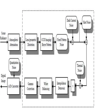
The CCD digital camera converts the irradiance, the photons coming into the imaging sensor, to electrons and finally to bits. See Figure 3 for the imaging pipeline of CCD camera. There are five primary noise sources as stated in [25], namely fixed pattern noise, dark current noise, shot noise, amplifier noise and quantization noise. These noise terms are simplified in [54]. Following the imaging equation in [54], we propose the following noise model of a CCD camera

I = f(L + ns + nc) + nq, (4)

(5)

I

nternational

J

ournal of

I

nnovative

R

esearch in

S

cience,

E

ngineering and

T

echnology

where I is the observed image brightness, f(·) is camera response function (CRF), ns accounts for all the noise components that are dependent on irradiance L, nc accounts for the independent noise before gamma correction, and nq is additional quantization and amplification noise. Since nq is the minimum noise attached to the camera and most cameras can achieve very low noise, nq will be ignored in our model. We assume noise statistics E(ns) = 0, Var(ns) =

Lσ2s and E(nc) = 0, Var(nc) = σ2c. Note the linear dependence of the variance of ns on the irradiance L.

V. DEPTH-GUIDED MULTI-VIEW IMAGE DENOISING

In this section, we present a novel method for denoising multi-view images given depth map estimation. Leveraging multi-view data, our method addresses two key challenges in single image denoising. First, multi-view images provide more measurements for noise cancelation, thereby enabling denoising patches that are non-repetitive within a single image. Second, we use depth-induced constraints among different views during patch matching, thereby improving the patch grouping accuracy in the presence of large noise.

Given multiple images, we choose one of them as a reference image, I1 for example.2 Consider one image patch bp (say 8x8) centred at pixel p in the reference image. We call this patch a reference patch. To denoise this reference patch, we search for patches that are similar to bp in all the input images, including the reference image itself. One way to achieve this goal is to compare the reference patch to all other patches, using a distance metric such as L2 norm. Such an approach however is susceptible to large image noise. The inaccuracy in patch grouping lowers the performance of image denoising. In practice, perfect patch matching is unobtainable as the noiseless image is unknown. However, we can improve the accuracy of patch matching using multi-view images as follows. When deciding whether a patch A1 is similar to a patch B1 in the reference image I1, we find their corresponding patches A2 and B2, respectively, in the second image I2 using the depth map. If A1 is similar to B1, A2 should also be similar to B2. Additionally, if we have more views, we have more measurements to verify whether A1 and B1 in the reference view are indeed similar. Specifically, we compute the similarity measure between patches bp and bq at locations p and q in the reference view as follows. We sum up the distances between patch pairs in all views that correspond to bp and bq:

Where Wm(p) is the warped location of pixel p from the reference image I1 to image Im using its depth, and bWm(p) is the patch centred at Wm(p) in image Im. Under this notation, W1(.) is the identity warp for the reference image I1 itself. Using (bp; bq) in Eq. as a metric, we can select K most similar patch locations for each patch in the reference image. After warping these K locations to all other M -1 views, we collect a group of KM similar patches for noise reduction.

Joint Multi View Patch Denoising:

Given the KM patches q=1 with similar underlying image structures, we now seek to remove their noise. Let the size of each patch be S x S = D; We treat each patch bq as a D-dimensional vector.3 We explore two methods for denoising: PCA and tensor analysis.

Since all the patches in the set have similar underlying image structures, we assume that their noiseless patches lie in a low dimensional subspace, centred at u0 and spanned by bases d=1. Let bq be the noiseless patch for patch bq:

(6)

I

nternational

J

ournal of

I

nnovative

R

esearch in

S

cience,

E

ngineering and

T

echnology

between noisy patches and denoised patches:

Finding Dimensionality C In practice, we need to determine the subspace dimension C. One choice is to use a fixed value, e.g., C = 1. However, different groups of patches require different numbers of principal components for best reconstruction, as shown in Figure. In general, too many components tend to introduce noise in the results and too few components tend to over-smooth the results. We propose a new way of choosing the dimension of the subspace for each patch stack that is adaptive to the underlying image structure. Our basic idea is that if we choose the right dimension for the subspace, the average squared residuals between noisy patches and denoised patches should be very close to the noise variance. Recall that we have KM patches, each having D pixels, and the average residual errors (scaled by variance) is

The singular values of the matrix B0. We therefore look for C such that Eq. (8) is closest to 1. Since Eq. (8) monotonically increases as C decreases from D to 1, a binary search can be used to quickly find an optimal C.

Patch Denoising using Tensor Analysis

Inspired by its successful application in modelling textures [21], we have also explored using tensor analysis for patch denoising. Specifically, rather than stacking patches from different images in a single matrix, we put patches from the same image in a stack, and view the patches from multiple images as a multi-dimensional array. Let this array be B and [B] i ; k ; m be the intensity of pixel i in the patch k in the view m. Since all the patches are similar, we assume that the underlying noiseless patch array B^ lie in a multi-linear subspace centred at u0 and spanned by bases.By applying the patch grouping and patch denoising to each patch in input images, we can denoise all of them; We now use the denoised patches to form denoised images. Each pixel is often covered by several denoised patches. To determine the value of a particular pixel in a denoised image, we take a weighted average of denoised patches at this pixel. The weight reflects our belief in the likelihood that the denoised patch resembles the true underlying noiseless image. Since the denoised patch is computed from the PCA or tensor analysis, a lower dimension of the subspace suggests less image structure variation in the patch collection and the noise has a better chance to be cancelled out.

VI. RESULTS

(7)

I

nternational

J

ournal of

I

nnovative

R

esearch in

S

cience,

E

ngineering and

T

echnology

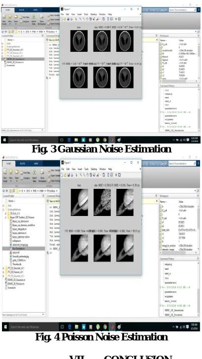
Fig. 3 Gaussian Noise Estimation

Fig. 4 Poisson Noise Estimation VII. CONCLUSION

In this work a novel image denoising algorithm is presented based on the nonlocal noise estimation, exploiting the spatial redundancy present in natural images. A low dimension signal subspace is used to group the similar patches in a data matrix. The multiple regression theory is than employed to calculate the model noise. The noisy image is restored using patch based restoration and the final image is obtained by hypothesis averaging. The simulated experiments suggest comparatively better or equivalent performance of the proposed algorithm comparing to some state of the art image denoising methods.

REFERENCES

[1] E. P. Bennett and L. McMillan. Video enhancement using per pixel virtual exposures. In SIGGRAPH, 2005. [2] A. Buades, B. Coll, and J. M. Morel. A review of image denoising algorithms, with a new one. Simulation, 4, 2005. [3] J. Chen and C.-K. Tang. Spatio-temporal markov random field for video denoising. In CVPR, 2007.

[4] V. Cheung, B. J. Frey, and N. Jojic. Video epitomes. IJCV, 76(2), 2008.

[5] K. Dabov, A. Foi, and K. Egiazarian. Video denoising by sparse 3d transform-domain collaborative filtering. In Proc. 15th European Signal Processing Conference, 2007.

[6] K. Dabov, R. Foi, V. Katkovnik, K. Egiazarian, and S. Member. Image denoising by sparse 3d transform-domain collaborative filtering. TIP, 16:2007, 2007.

[7] M. Elad and M. Aharon. Image denoising via learned dictionaries and sparse representation. In CVPR, 2006.

(8)

I

nternational

J

ournal of

I

nnovative

R

esearch in

S

cience,

E

ngineering and

T

echnology

[9] G. Healey and R. Kondepudy. Radiometric ccd camera calibration and noise estimation. TPAMI, 16(3):267–276, 1994.

[10] Y. S. Heo, K. M. Lee, and S. U. Lee. Simultaneous depth reconstruction and restoration of noisy stereo images using non-local pixel distribution. In CVPR, pages 1–8, 2007.

[11] V. Kolmogorov and R. Zabih. Multi-camera scene reconstruction via graph cuts. In ECCV, 2002. [12] K. N. Kutulakos and S. M. Seitz. A theory of shape by space carving. IJCV, 38(3):199–218, 2000.

[13] L. D. Lathauwer, B. D. Moor, and J. Vandewalle. On the best rank-1 and rank-(r1;r2; : : : ;rn) approximation of higher- order tensors. SIAM J. Matrix Analysis and Applications, 21(4):1324– 1342, 2000.

[14] S. Lyu and E. P. Simoncelli. Statistical modeling of images with fields of gaussian scale mixtures. In NIPS, 2006. [15] R. Ng. Fourier slice photography. ACM Trans. Graph., 24(3), 2005.

[16] M. Okutomi and T. Kanade. A multiple-baseline stereo. TPAMI, 15(4):353–363, 1993.

[17] S. Roth and M. J. Black. Fields of experts: A framework for learning image priors. In CVPR, pages 860–867, 2005.

[18] D. Scharstein and R. Szeliski. A taxonomy and evaluation of dense two-frame stereo correspondence algorithms. IJCV, 47(1- 3), 2002. [19] M. F. Tappen, C. Liu, E. H. Adelson, andW. T. Freeman. Learning gaussian conditional random fields for low-level vision. In CVPR, pages 1–8, 2007.

[20] V. Vaish, M. Levoy, R. Szeliski, C. L. Zitnick, and S. B. Kang. Reconstructing occluded surfaces using synthetic apertures: Stereo, focus and robust measures. In CVPR, pages 2331– 2338, 2006.