Model Discrimination Using Bounded Error Estimation Approach

(1)

Abstract

CHATTOPADHYAY, SOMRITA. Model Discrimination Using Bounded Error Estimation Approach. (Under the direction of Stephen Campbell.)

(2)

(3)

Model Discrimination Using Bounded Error Estimation Approach

by

Somrita Chattopadhyay

A thesis submitted to the Graduate Faculty of North Carolina State University

in partial fulfillment of the requirements for the Degree of

Master of Science

Mathematics

Raleigh, North Carolina

2015

APPROVED BY:

Mansoor Haider Negash Medhin

(4)

Dedication

To my parents.

(5)

Biography

(6)

Acknowledgements

I would like to thank my advisor Dr. Campbell for his excellent guidance and endless patience during the course of my Masters research. His valuable suggestions have not only helped me to achieve success in my research work, but have also contributed immensely towards my professional and personal growth.

I also acknowledge Dr. Haider and Dr. Medhin; their valuable inputs and constant support towards my degree completion kept me calm as well as motivated throughout my graduate studies.

(7)

List of Tables

(10)

List of Figures

Figure 3.1 Mapping from state space Rn _{to data space} _Rm _{using the function}

y(t) =g(x(t), p)[19] . . . 21

Figure 3.2 Feasibility of boxes using SIVIA . . . 25

Figure 3.3 Parameter Estimation Algorithm[19] . . . 27

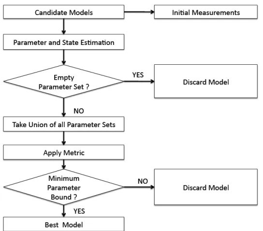
Figure 3.4 Block Diagram for Model Discrimination method . . . 28

Figure 4.1 State Estimation of the Reference Model for 6 different initial con-ditions. X-axes represent time, Y-axes represent bounded state out-puts. The red and black colored lines represent the lower and upper bounds of the state intervals. . . 33

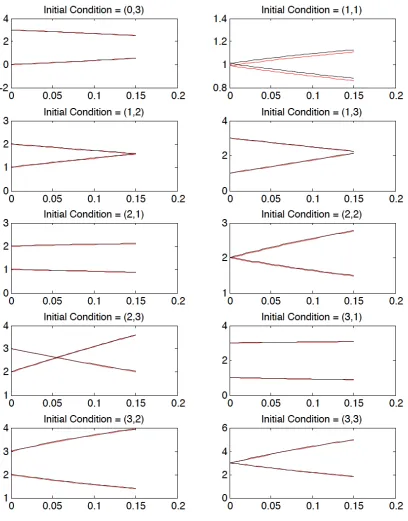
Figure 4.2 State Estimation of the Reference Model for 10 different initial con-ditions. X-axes represent time, Y-axes represent bounded state out-puts. The red and black colored lines represent the lower and upper bounds of the state intervals. . . 40

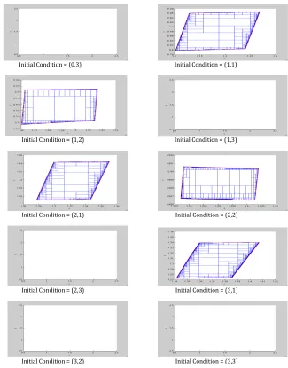
Figure 4.3 Parameter Estimation of the Michaelis-Menten Model for 10 different initial conditions. X-axes represent the parameter space of c and Y-axes represent parameter space of f. . . 42

Figure 4.4 Parameter Bound for Model 1 . . . 45

(11)

Chapter 1 Introduction

1.1 Overview

Systems biology is an emerging research field that deals with quantitative representa-tion of dynamic biological systems. Systems biologists mainly focus on understanding biological processes at system level by studying the interactions between individual com-ponents of the system and representing them in a mathematical framework. In recent years, it has become a groundbreaking scientific approach towards developing accurately predictive biological models, which have the potential to bring advancement in the fields of medicine, agriculture, ecosystems and food science[8]. Like engineers, systems biolo-gists first develop an overall understanding of a particular system and then apply that knowledge to control it. Thus, systems biology is not only a scientific field, but also an engineering discipline[28].

(12)

predictive power [13]. Analyzing, representing, manipulating and integrating such data requires application of ideas from diverse areas of electrical and computer engineering like artificial intelligence, signal processing, control theory and many more. Thus systems bi-ology is highly reliant on computational and analytical tools developed by electrical and computer engineers.

From medicine and environmental science to alternative fuel technology and agri-culture, systems biologists are bringing revolutionary changes [28]. The most eminent impact will be in the health-care sector by means of new drug discovery [6] and innovative treatment of complex diseases like cancer, dementia, aging[8] and neurological problems [38]. It is also leading to the development of bio-fuels and artificial algae design to pro-cess carbon-dioxide to reduce power-plant emission [28]. Systems Biology also provides a platform for the foundations of Synthetic Biology, another emerging research field, which deals with design and construction of new biological systems that are not available naturally.

The work described in this thesis focuses on finding the most appropriate model among many dynamic models used to represent the same biological process. A set based approach has been developed for this purpose. The algorithm has been applied on two dif-ferent test cases and the results obtained show that even in presence of non-deterministic uncertainty, our method can outperform the traditional approaches designed for model discrimination.

1.2 Motivation

(13)

ex-perimentally or observed. So, the need arises for representing biological processes in a framework of mathematical equations. For any given system, there can be a number of equation sets with unique characteristics that distinguishes one model from the other. This gives rise to situations where several models can explain the available set of data equally well. As these mathematical models are mainly used to predict and control the future behavior of the given biological process, a sufficiently accurate model with less complexity is required to understand the actual underlying phenomenon. The question now becomes how to find the best suited model out of different equally likely hypotheses. This gives rise to different model discrimination theories.

In this paper, we have aimed at developing a set based model discrimination ap-proach. Usually, most of the classical methods treat uncertainty associated with data sets as statistically defined noise or require a detailed priori knowledge about the system parameters. However, this type of assumption is not appropriate for biological systems. Uncertainty in these nonlinear systems can arise from a variety of factors, such as -measurement error, non-stringent experimental setup, etc. Moreover in most cases, suf-ficient experimental data is not available at the beginning of modeling. Thus, heuristic approaches, based on experience or intuition, are also not applicable. Our method char-acterizes errors in the data by simple sets such as interval boxes, ellipsoids, zonotopes, etc [16]. Uncertainty associated with biological systems are more aptly represented by a continuous range of values. The method is very appealing, because our proposed algo-rithm analyzes entire sets, instead of just checking some finite amount of distinct points. This gives us a better understanding of the true dynamics of the system.

(14)

measurements with high uncertainty are available. The work presented in this document is based on an improved parameter estimation algorithm [20] developed over the works of Raissi [30] and Jaulin [11]. Thus our approach for model discriminication handles the problem of increased computational time and availability of only sparse, discrete data in a better and concrete manner by employing techniques like parallelization and preprocessing.

1.3 Thesis Contribution

1.3.1 Intellectual Merit

The intellectual merit of this research work is described below :

A technique has been developed to distinguish competing model hypotheses, all rep-resenting the same biological activity. This is achieved without imposing any unrealistic assumption or probabilistic characterization on the data sets. The uncertainties associ-ated with the data are supposed to be bounded without any other assumption on their distribution.

1.3.2 Broader Impacts

(15)

strategy, one needs to choose the best representative model of the particular situation. Finding the best representative model is not a trivial task. The contribution of this research lies in solving such problems in a more concrete and realistic manner, without taking into consideration any probabilistic assumption. Thus, the work presented in this thesis will prove to be an important tool for system biologists in the future. This work will not only be beneficial for modeling of biological systems, but can also be applicable for other control systems.

1.4 Thesis Organization

The entire thesis is divided into five chapters.

Chapter 1 gives us an overview of the field ’Systems Biology’ and its application in today’s world. It also describes in brief the contribution of this research.

Chapter 2 explains the foundation, terminologies and concepts used for this research work. It also discusses some of the other work conducted in the area of model discrim-ination and points out how the work presented here is different from the traditional approaches.

Chapter 3 gives a detailed description about our approach towards developing a model discrimination algorithm for biological systems.

Chapter 4 mainly illustrates the results of our proposed method. Outcome of our algorithm is demonstrated by its application on two different case studies.

(16)

Chapter 2 Background

This chapter discusses the recent state of art in the field of model discrimination for biological systems and advantages of our method over others.

2.1 Overview

(17)

models can explain the available set of data equally well. As these mathematical models are mainly used to predict and control the future behavior of the given biological process, a sufficiently accurate model with less complexity is required to understand the actual underlying phenomenon. In the early phase of mathematical modeling, while establishing the interactions and reactions in the pathway, mathematical descriptions of the competing hypotheses can be used to verify whether or not these hypotheses are viable by com-paring with the experimental data that has been obtained. The question now becomes how to find the best model out of different equally likely hypotheses. This becomes a very compelling application for model discrimination, particularly since the experimental data that has been obtained contains some sort of uncertainty.

Accurate models are required for understanding, predicting and finally controlling biological systems. Adding new features to these models are, thus, often necessary. But this gives rise to increased complexity in terms of increased number of parameters. As these parameters play an important role in influencing the model’s dynamics, efficient parameter estimation algorithms are crucial to discriminate between different candidate models.

(18)

independent and identically distributed, usually Gaussian with zero mean and variance

σ2 _{or require detailed a-priori knowledge about the noise characteristics. Thus,} proba-bilistic and heuristic approaches, based on experience or intuition, are not appropriate for biological systems. Moreover, the classical approaches are deficient as they evaluate a finite number of points in the parameter space. But, uncertainty in biological systems is more aptly represented by a finite range of continuous values where true dynamics of the system lie [30].

In this chapter, we discuss the common methods of model discrimination and some of the drawbacks associated with them. We also explain why our discrimination approach is aptly suited for biological systems.

2.2 State of Art

A majority of the classical approaches in parameter estimation and model discrimination usually focus on finding the difference between the experimental data and the predicted model output. This is usually achieved by employing weighted least square methods or maximum likelihood functions. These methods usually employ Fisher Information Matrix and associated A-, D- or E- optimality [9],[3],[39]. These approaches usually give rise to solving non-convex optimization problems, which are very difficult to solve. Thus, locally optimal solutions with some desired global properties are searched for and this, at times, may lead to unsatisfying parameter estimates due to non-convergence to a global optimum in finite time [21],[23],[17].

(19)

be distinguished. However, this method depends on the development of a controller in laboratory, which may turn out to be a difficult task.

Dominik et al. in [34] explains a KL- optimality criterion for model discrimination. It calculates the number of optimal measurement location and time points instead of continuous design. It also gives the optimal initial condition and optimal perturbation to the system. This method employs a fitting technique and uncertainty associated with experimental data is assumed to have a fixed probability distribution.

Literature shows that model selection is also approached using various types of Kalman filters. These methods basically tackle the above stated problem from a control theory point of view by using state observers. One of the recent works is presented in [15] where the authors have developed a constrained hybrid extended Kalman filtering algorithm that can handle sparse and noisy data, applied to large parameter spaces. However, the Kalman filter is not generally an optimal estimator in a non-linear setting. Also, if the initial conditions are not close-by,the filter may end in an estimate whose mean is different from the true mean. In such cases, these methods produce unreliable results.

[22] describes discrimination method of multiple model candidates based on Akaike’s Information Criterion. Problem of model lumping while applying RSOS methods is overcome using the AWDC criterion which reduces the number of experimental designs in the early stage of model identification and thus, reduces the overall cost of the system. AIC minimizes KL-distance between model and truth. The best model is the one with lowest AIC. This is a relative likelihood approach.

Several methods have also applied semi-definite programming to solve the problem of model discrimination in a convex optimization framework [25],[27].

(20)

trend of the state or state variables behavior. However, models chosen are deterministic and thus, maximizing the upper bound can not guarantee discrimination.

[25] proposes three different approaches to maximize the output between different can-didate models. Those are (a) best initial condition is determined which discriminates the models the most. (b) Best input distribution is chosen to maximize the difference be-tween model outputs. (c) Best initial condition is modified with structural modifications to achieve maximum difference in model outputs. Here the SOS technique has been used and a Bayesian approach is followed. Time series data having maximum information (how measurements are spaced in time, how many are needed, etc.) is collected. In these methods, same input or initial conditions are taken and outputs of different patterns are generated. Then the same conditions are applied to the actual physical system and the model whose pattern differs hugely from the actual system is discarded. But, only de-terministic models that do not consider noise measurements directly are used here. The authors have tried to make the outputs of the two models as distant as possible so that even a noisy measurement has a good chance of discriminating between them.

(21)

dimensional problems or where large data samples are available.

In this type of mathematical modeling, one of the most important and complicated tasks is to characterize the uncertainty associated with the corresponding biological pro-cesses. In most of the works described above, variation associated with data measure-ments are modeled as statistically defined noise i.e. the errors produced due to noise are assumed to be independent and identically distributed, usually Gaussian with zero mean and varianceσ2. However, non-linear and poorly understood system dynamics make this characterization inappropriate for biological processes. In these cases, it is preferable to bound the error associated with the models by simple range of values than any statis-tical assumption. Moreover, the classical approaches are deficient as they evaluate at a finite number of points in the parameter space. Thus, uncertainty in biological systems is more aptly represented by a a continuous range of values where the true dynamics of the system lie [30].

Recent works in this field have focused on characterizing noise present in biological systems in a bounded error context. Set-based approaches for parameter estimation and model discrimination have started receiving immense attention since the last decade. The only assumption, considered in these methods, is that we have prior knowledge about the upper and lower bounds of the parameter sets and measurement errors, but no hypoth-esis regarding the error distribution in these sets is known. Sophisticated approaches, nowadays, employ interval analysis and semi-definite programming to address the same problem.

(22)

is to determine an outer approximation of the parameters which are consistent with the available data (called SCP - set of consistent parameters). To efficiently outer bound the set of consistent parameters, infeasibility certificates are obtained by SDP. Model falsification is done by showing SCP to be empty. This method aims at overcoming the problems of noisy data and system’s non-convexity with the help of bounded measure-ment error.

Our method also characterizes errors in the data by simple sets such as interval boxes, ellipsoids, zonotopes, etc [16]. In our work, we bound the uncertainty associated with the system by a continuous range of values. The method is very appealing, because our proposed algorithm analyzes entire sets, instead of just checking a finite number of distinct points. This gives us a better understanding of the true dynamics of the system. The main concept used by both the Interval Analysis and SDP methods is that the parameter space is bounded and not defined by any distribution. However, we have chosen Interval Estimation method over SDP because of the following reasons

-• Firstly, other set-based approaches, including SDP, mainly aimed at model

invali-dation rather than model discrimination. These approaches discarded the models having empty SCP. However, no solution has been provided for cases where more than one model has feasible parameter sets. Our method addresses this issue by designing a metric which can discriminate between models having non-empty SCPs. To our knowledge, this problem has not been investigated previously.

• Secondly, interval estimation method is based on the use of validated methods for

(23)

the problem has a unique solution and thus, a guaranteed enclosure of the solution can be derived. However, the SDP approaches employ some relaxation criteria to solve the non-convex problems. This relaxed version makes sure that there are no false negatives in the solution i.e. no feasible parameterization is lost. However, the result may contain false positives [31]. This may end up producing some inaccurate solutions. This means that there could be cases in which the actual solving problem would allow us to invalidate a model, while solving the relaxed version does not. However, if the relaxed version is infeasible, this guarantees that the actual non-convex problem is infeasible as well, and hence that the model is inconsistent with the experimental data. Interval method may also produce false positives. However, as stated previously, our aim is not to invalidate a model; we discriminate between the models. Thus, presence of false positives do not affect our solution vigorously. Moreover, we recursively divide the interval boxes until the user defined tolerance is reached. As the boxes get smaller and smaller, the occurrence of false positives also decrease. This makes our approach more robust.

(24)

2.3 Our Approach

In this paper, we have utilized the interval analysis method[24] to solve the model dis-crimination problem in a set based framework. Interval boxes are used to bound error associated with the data. We have represented the models in terms of ordinary differ-ential equations. Our novel approach is based on the works in [11], [30] and [20]. If two or more model variants describe the available experimental data, a new experiment must be designed to discriminate between the hypothetical models. We basically want to see how well the old model describes the new data set. The key idea is to find an in-put profile that maximizes the difference of the outin-puts of the competing models. Once we have designed the new data set, the states and parameters of the models are first estimated using Extended mean Value (EMV) theorem and Set Inversion Via Interval Analysis (SIVIA) approach and, then the uncertainty associated with those parameters are checked. Model discrimination can then be achieved by comparing the parameter bounds of the competing models. The model with most consistent parameter set is chosen as the best model.

2.4 Discussion

(25)

(26)

Chapter 3 Methodology

This chapter introduces all the important concepts used in the paper and gives a detailed description of our approach to find the best model among a set of candidate models.

3.1 Overview

(27)

3.2 Biological Modeling

Many biological systems can be modeled by using a set of ordinary differential equations. The general form of a model can be represented as

-˙

x(t) =f(x(t), p) (3.1)

y(t) =g(x(t), p), x(t0)∈X0 (3.2) where x∈ Rn _{denote the n-dimensional state vector,} _y_∈ _Rm _{denote the m-dimensional}

measured output vector and p∈ Rp _{are the p model parameters. The initial conditions}

x(t0) are supposed to belong to an initial “box” [X0], the notion of ”box” being described in the following.

An interval vector (or box) [X] is a vector with interval components and may equiv-alently be seen as a Cartesian product of scalar intervals: [X] = [x1]×[x2]×...×[xn],

where [xi] represents the interval set xi ≤xi ≤xi. The set of ndimensional real interval

vectors is denoted by IRn_.

Time is assumed to belong to [0, tmax]. The functions f and g are real and finite on

M, where M is the open set of Rn _{such that} _x₍_t₎ _∈_M _{for every} _t_∈ _[0_{, t}

max]. Moreover

the functionf is assumed to be at leastk-times continuously differentiable in the domain

M. The structures of functionsf and g depend on the modeling frameworks required to describe specific biological systems.

The output error is assumed to be given by:

v(ti) =y(ti)−ym(ti), i= 1,2, ..., N. (3.3)

(28)

solution of a differential equation. v(t) and v(t) are known lower and upper bounds for the acceptable output errors. Such bounds may, for instance, correspond to a bounded measurement noise. The integer N is the total number of sample times.

Interval arithmetic is used to compute guaranteed bounds for the solution of (3.1) and (3.2) at the sampling times {t1, t2, ..., tN}.

3.3 Problem Statement

In this work, our goal is to discriminate between two different mechanisms that produce similar biological phenotypes. We develop an approach that investigates transitions to the steady states and uncertainty to discriminate between competing mechanistic hypotheses. We do this by exploring the consistency of estimated uncertain parameters over uncertain experiments that explore model dynamics.

(29)

3.4 Interval Analysis

Interval arithmetic is a method of bounding measurements and rounding off errors in mathematical computations. Interval analysis was initially developed to assess the nu-merical errors resulting from the use of finite-precision arithmetic. It now makes it possi-ble to obtain guaranteed solutions to standard engineering propossi-blems such as computing solution of non-linear system of equations or all global minimizers of a cost function, or computing sets guaranteed to contain all solutions of sets of nonlinear inequalities.

This approach can characterize the uncertainty associated with biological systems better than other approaches which are based on statistical assumptions. Thus, due to limited accuracy of available experimental data, interval analysis [24] is becoming an essential tool for biological modeling.

In the following section, we present some basics tools of interval arithmetic and two popular algorithms to compute the outer approximation of sets of arbitrary shape.

3.4.1 Basic Tools

A real interval [x] = [x, x] is a closed and connected subset of R where x represents the lower bound of [x] and xrepresents the upper bound of [x]. The width of an interval [x] is given by w(x) =x−x, and its midpoint by m(x) = (x+x)/2.

Two intervals [x] and [y] are considered equal if and only if x=y and x=y. We can also extend real arithmetic operations to intervals [24].

Arithmetic operations on two intervals [x] and [y] can be defined by :

(30)

An interval corresponding to [u]◦[v] for the first three operators can be easily obtained by :

[x] + [y] = [x+y, x+y], [x]−[y] = [x−y, x−y],

[x]∗[y] = [min(xy, xy, xy, xy), max(xy, xy, xy, xy)].

However, for division, when 06∈[y] ,

[x]/[y] = [min(x/y, x/y, x/y, x/y), max(x/y, x/y, x/y, x/y)].

and extended intervals have to be introduced, when 0∈[y].

Thus, the interval counterpart of a real-valued function is an interval-valued function defined as :

f(|x|) = [{f(x) |x∈[x]}],

where [S] is the interval hull of S, i.e., the smallest interval containing it.

Interval counterparts to continuous elementary functions can also be obtained easily. For monotonic functions, only computations on bounds are required :

exp([x]) = [exp(x),exp(x)],

log([x]) = [log(x),log(x)], if x >0

(31)

as :

[x]2 =



  

  

[0,max(x2_{, x}2_)]_, _{if 0}_∈_[_x_] [min(x2_{, x}2₎_,_max(_x2_{, x}2_)]_, _else

For more complicated functions, it is no longer possible to evaluate the interval coun-terparts easily and, thus the inclusion functions were introduced. An inclusion function [f](.) for a function f(.) defined over a domainD ⊂R is such that the image of an inter-val by this function is an interinter-val, guaranteed to contain the image of the same interinter-val by the original function:

∀[x]⊂ D, f([x])⊂[f]([x]). (3.4) When the inclusion in (3.4) becomes an equality, the inclusion function is minimal.

This inclusion function is convergent if limw([x])→0w([f]([x])) = 0, where w is the width of the interval [x], and inclusion monotonic if [x]⊂[y] implies [f]([x])⊂[f]([y]).

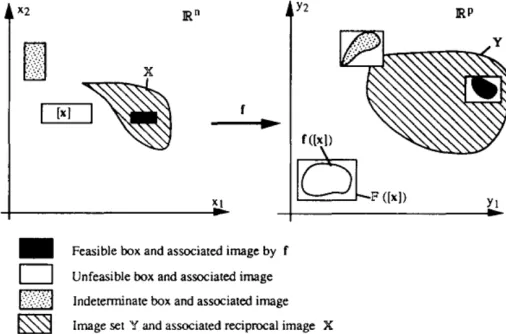
Figure 3.1: Mapping from state space Rn _{to data space} _Rm _{using the function} _y₍_t_{) =}

g(x(t), p)[19]

(32)

model linear as well as non-linear systems in a bounded error context.[20],[19]. In Fig-ure 3.2, it is shown that the model function g maps a state interval box [x] to another image, g([x]), in the output data space, Rm_{. Here, [x] represents the Cartesian product}

of n scalar intervals i.e. [x]=[x1]×[x2]×...×[xn], where [xi] represents the interval set

x_i ≤ xi ≤ xi. [g] is a unique minimum inclusion function that maps x to the smallest

box that encases the image, g([x]). As in practical scenarios, these minimum inclusion functions are not always attainable, an approximation is made such that [g]([x])⊂G([x]).

3.4.2 Inverse Image Evaluation (Set Inversion)

The SIVIA algorithm (for Set Inverter Via Interval Analysis) [11] is dedicated to the characterization of sets defined by :

S={u∈U |Φ(u)∈[y]}= Φ−1([y])∩U, (3.5) where [y] is known a priori,U is an a priori search set foruand Φ a nonlinear function not necessarily invertible. (3.5) involves computing the reciprocal image of Φ and is known as a set inversion problem which can be solved using the algorithm Set Inversion Via Interval Analysis (denoted SIVIA). The algorithm SIVIA [11] is a recursive algorithm which explores the entire search space without losing any solution and ensures a guaranteed enclosure of the solution set S. The algorithm recursively builds two unions of non-overlapping boxes (subpavings)S and S such that :

(33)

The inner enclosure S is composed of the feasible boxes. To show that a box [u] is feasible it is sufficient to prove that Φ([u]) ⊆ [y]. Reversely, if Φ([u]) ∩ [y] = ∅, the box [u] is unfeasible. Otherwise, no conclusion can be reached and the box [u] is indeterminate. The latter is then bisected and checked again until its size reaches a user-specified precision threshold > 0. This ensures that the SIVIA algorithm terminates after a finite number of iterations.

3.4.3 Direct Image Evaluation

Another popular algorithm using the interval analysis concept is Direct image evaluation. This is the characterization of

Y =f(X) (3.7)

whenX is a known set and f a known function. This task is usually quite complex. The algorithm IMAGESP, again based on interval analysis, builds a sub-paving Y such that

Y ⊂Y when Y is an outer approximation of the set Y, X is itself a sub-paving and an inclusion function [f] is available for f. A subpaving of a box [x] ∈Rn _{is a union of}

non-overlapping subboxes of [x] with non-zero width. Two boxes in the same subpaving may have a non-empty intersection if they have a boundary in common, but their interiors must have empty intersection. IMAGESP consists of three steps :

1. Firstly, all boxes in X are bisected in order to obtain a sub-paving X0 consisting only of boxes of width less than a pre-specified precision parameter .

(34)

3. Finally, all boxes in Y are merged into a new sub-paving Y.

Y is guaranteed to contain Y. The precision of the approximation is controlled by an user-defined threshold >0.

3.5 Extended Mean Value Theorem and Set

Inver-sion via Interval Analysis

The Extended Mean Value theorem (EMV) is a method to find a valid solution of eqs. (3.1) and (3.2) at an initial condition x0 = x(t0) using bounded error context. This algorithm produces a enclosure of the state estimate at each time step, ensuring that all possible solutions are retained. This is done by using Taylor expansion method [24, 26]. The Taylor expansion is evaluated using the method explained in [29] with the help of mean value theorems [1] and matrix preconditioning.

EMV uses interval analysis and generates state intervals. Whenever a state value is generated at a time where previous measurements are available, SIVIA is employed to compare those two values. If we have a functionh, output y and an initial condition x0, SIVIA is used to find a solution of x=h−1(y). The state space x is iteratively searched for guaranteed enclosure of the solution space. In the solution space, the feasible boxes are surrounded by the set of indeterminate boxes. The parameter boxes are classified as follows

-• If the state intervals are completely contained within the data measurements, the

parameter subset is feasible.

• If the state intervals span outside but still contain part of the data measurement,

(35)

• If the data measurement is completely outside the state interval the parameter

subset is unfeasible.

This basic concept of the set inversion algorithm can be illustrated using a simple example :

Let us consider, the set X = f−1([4,9]) where f(x1, x2) = x12 +x22. As explained above, there can be the following three scenarios :

• Since [2,1]2_{+ [4}_,_5]2 _{= [4}_,_{1] + [16}_,_{25] = [20}_,_{26] does not intersect the interval [4}_,_9], the box [−2,1]×[4,5] is outside X and considered unfeasible.

• Since [0,2]2 + [2,1]2 = [0,4] + [4,1] = [4,5] is completely inside the interval [4,9], the box [0,2]×[2,1] is considered feasible.

• Since [1,1]2_{+ [0}_,_2]2 _{= [1}_,_{1] + [0}_,_{4] = [1}_,_{5] is partially inside the interval [4}_,_{9], the} box [−2,1]×[4,5] is considered indeterminate.

Below, we give a pictorial representation of the SIVIA algorithm :

(36)

3.6 Parameter and State Estimation

The parameter and state estimation approach used in this work are originally developed by Raissi [30] and Jaulin [11] and later on parallelized by Skylar Marvel[19]. This esti-mation method efficiently combines the EMV and SIVIA algorithms for evaluating the parameter boxes and checks whether each box produces trajectories consistent with the available data or not.

The algorithm starts with an unclassified parameter box and Extended Mean Value algorithm is applied on it. Whenever a data measurement is available during the execu-tion of the EMV algorithm, the corresponding state output is compared to the bounded measurement using SIVIA. The unfeasible sets are immediately discarded. For all other cases the EMV algorithm will run until the final time and the parameter box is then classified. Feasible boxes are retained and other boxes are regarded as indeterminate. When a box is found to be indeterminate, the longest edge is compared to a user defined width, epsilon. If the longest box edge is larger than epsilon, the indeterminate box is bisected and each resulting box is reevaluated. The PE algorithm runs until every pa-rameter box has been classified as feasible, unfeasible, or is small enough to be classified as indeterminate. Block diagram of this algorithm is shown in Figure 3.3.

3.7 Model Discrimination

(37)

parame-Figure 3.3: Parameter Estimation Algorithm[19]

(38)

models. Single parameter values are compared using the width of the uncertainty for the parameter of interest, e.g. Ppi = pi−pi, where pi denotes the upper bound, pi the

lower bound of the selected parameter over all the feasible parameter sets for all the ini-tial conditions. This parameter bound represents the maximum amount of uncertainty associated with the selected parameter of a particular model. More the width of the pa-rameter bound, more is the noise associated with that papa-rameter. So, smaller papa-rameter bound of a model implies that the parameter of that particular model is more consistent. The model with minimum parameter bound, thus, represents the reference model most accurately and is chosen as the most suitable model i.e. the best among the competing hypotheses.

A high level block diagram of our model discrimination approach is shown in Fig 3.4.

(39)

3.8 Discussion

This chapter has focused on a detailed description of our model discrimination approach. We have also provided brief overviews of the relevant algorithms. Our framework is en-tirely based on the works done by Skylar et al. [19]. Thus, we have used a parallelized parameter estimation algorithm which proved to be faster than traditional PE algorithms. Previous model discrimination algorithms, rather than discrimination, aimed at invali-dating the models with empty feasible parameter sets. However, our approach can not only invalidate the models with empty parameter sets, but can also make discrimination among the candidate models with feasible parameter sets.

(40)

Chapter 4 Results

(41)

4.1 Case Study I

The first case studies two different Lotka-Volterra predator-prey population models. This kind of model describes the population dynamics of two species. We assume that both the species are competing for the same food and the food supply is limited. Each species grow according to its own capacity in absence of the other. This can be modeled assuming logistic growth of each species[35]. However, the problem starts when they confront each other. We assume that the growth rate for each species reduces due to this conflict. In our work, we have taken two specific models that incorporates these assumptions.

4.1.1 Model Discrimination Between Two Predator - Prey

Population Models

In both the models, the prey and the predator populations are denoted by x1 and x2. The general form of the predatorprey model is

-˙

x1 =p1x1−p2x12−p3x1x2 (4.1) ˙

x2 =p4x2−p5x22−p6x1x2 (4.2) where pi are the parameters reflecting the rates of population change of the predators

and the prey.

The parameters for our reference model are taken as: p1 = 3, p2 = 2, p3 = 2, p4 = 2, p5 = 1, p6 = 1. Data is generated by the EMV algorithm from this model and uncer-tainty is added to obtain bounded interval measurements.

(42)

data generated from the reference model.

For the candidate models, the known parameters are taken as

-• Model 1: p1 = 3, p2 = 2, p4 = 2, p5 = 1

• Model 2: p1 = 3, p2 = 1, p4 = 2, p5 = 1

4.1.2 Experimental Setup

The first step of our algorithm deals with generation of data measurements from the reference model. The measurements are simulated for 6 different initial conditions, (x1(0), x2(0)) = {(1,2),(1,3),(2,2),(2,3),(3,2),(3,3)} and for each set of initial con-dition, a 4th order Taylor expansion is used to obtained 30 data points. We run this experiment with a constant time step of 0.005 and α = 0.005. The bounded interval measurements (shown in Figure 4.1) are then obtained by adding ±0.01 uncertainty to all the generated state values.

The second step aims at finding the feasible parameter values of p3 and p6 for the candidate models corresponding to the data generated from the reference model. Here, we only use the bounded error measurements for the prey population i.e. y = x1.The initial intervals assumed for the parameters are as follows

-• Model 1: p3 = [1,3] and p6 = [0,2]

• Model 2: p3 = [1,3] and p6 = [0,2]

For both the models, the indeterminate boxes are bisected until the width is less than

= 0.00001.

(43)

(44)

The state and parameter estimation stage of our experiment is most time consuming. Thus, we ran the algorithm with either 1, 2, 4 or 8 threads. The average computation times with respect to each initial condition were 33.35, 15.48, 7.92 and 4.24 seconds for 1, 2, 4 and 8 threads, respectively. Observed decreases in computation time were factors of 2.15, 4.21 and 7.86 when increasing the number of threads from 1 to 2, 4 and 8, respectively.

4.1.3 Results and Analysis

The results for parameter estimation of candidate model 1 and 2 are displayed in the tables 4.1 and 4.2.

(45)

Table 4.1: Results of PE for Model 1

Initial Conditions Indeterminate set of p3 Feasible Set of p3 Indeterminate set of p6 Feasible Set of p6 (1,2) [1.936256, 2.063865] [1.936294, 2.063819] [0.941009, 1.060043] [0.941047, 1.060005] (1,3) [1.946128, 2.054740] [1.946174, 2.054687] [0.945365, 1.055259] [0.945419, 1.055198] (2,2) [1.953315, 2.046562] [1.953392, 2.046485] [0.9642486, 1.035720] [0.964302, 1.035667] (2,3) [1.961991, 2.038322] [1.962089, 2.038223] [0.9679641, 1.032402] [0.968048, 1.03231] (3,2) [1.957725, 2.042152] [1.957847, 2.042015] [0.9721679, 1.02787] [0.9722366, 1.027793] (3,3) [1.966384, 2.033607] [1.966552, 2.033439] [0.9754333, 1.024749] [0.9755554, 1.02462] Overall range of

(46)

Table 4.2: Results of PE for Model 2

Initial Conditions Indeterminate set of p3 Feasible Set of p3 Indeterminate set of p6 Feasible Set of p6 (1,2) [2.380584, 2.500030] [2.380607, 2.499984] [0.939163, 1.057167] [0.9391937, 1.057128] (1,3) [2.231399, 2.330024] [2.231422, 2.329971] [0.9434814, 1.051651] [0.9435348, 1.051589] (2,2) [2.864250, 2.878952] [2.864318, 2.878852] [0.9831924, 1.02911] [0.9836578, 1.029052] (2,3) [2.561820, 2.567054] [2.561897, 2.566932] [1.003822, 1.02456] [1.004516, 1.024482]

(3,2) [0, 0] [0, 0] [0, 0] [0, 0]

(3,3) [0, 0] [0, 0] [0, 0] [0, 0]

Overall range of parameter variation

(empty sets

(47)

4.2 Case Study II

Our second case study deals with two alternative reaction schemes - Henry mechanism and Michaelis-Menten mechanism. Both the schemes [31] represent the same chemical reaction in which an enzyme (E) reacts with a substrate (S) to form a complex (C) and gives the final product (P). The reactions are represented as

-• Michaelis-Menten Model: E+S−₎k*₋1

k2

C k3

−→E+P

• Henry Model: C −₎k*₋1

k2

E+S k3

−→E+P

where ki are the rate constants in both models. [32] gives detailed description about

the relevance of these models. In our work, we have discriminated these two schemes by capturing their transient phase behavior, as they are analytically indistinguishable during the steady state conditions.

4.2.1 Model Discrimination Between Henry and Michaelis-Menten

Mechanisms

The above reaction schemes can be modeled as 4-state models according to the law of mass action.

• Michaelis-Menten Model ˙

S =−k1ES+k2C ˙

C =k1ES−k2C−k3C ˙

E =−k1ES+k2C+k3C ˙

(48)

• Henry Model ˙

S =k1C−k2ES ˙

C =−k1C+k2ES ˙

E =k1C−k2ES+k3ES ˙

P =k3ES

These 4-state models can again be converted into 2-state models without any loss of generality by utilizing a conservation relationship satisfied by both the schemes. First we assume that the systems are dependent only on the concentrations of S and C. And we fix the total enzyme concentration E+C to a constant value 1 [31].

The above equations transform into the following two state forms

-• Michaelis-Menten Model ˙

S =−k1S+k2C+k1ES ˙

C =k1S−(k2+k3)C−k1ES • Henry Model

˙

S =−(k2+k3)S+k1C+ (k2+k3)ES ˙

C =k2S−k1C−k2ES

For simplicit, we take the substrate and the complex concentrations asx1 andx2 respectively. We then rewrite the above schemes into a general form as follows

-˙

x1 =−ax1+bx2+cx1x2 (4.3) ˙

(49)

We aim at invalidating the Michaelis-Menten model based on the uncertain measure-ments generated from the Henry model which we have considered to be the reference model in this case. The parameters for our reference model are taken as: a=k2+k3 = 2, b =k1 = 1, c =k2+k3 = 2, d =k2 = 1, e=k1 = 1, f =k2 = 1. Data is generated by the EMV algorithm from this model and uncertainty is added to obtain bounded interval measurements.

For the Michaelis-Menten model , we assume that the parameters -a, b, d, eare known. Our aim is to estimate the feasible parameter sets corresponding to c and f using the data generated from the Henry model. The known parameters for this model are taken as - a= 1.5, b= 1.3, d= 1.5 and e= 1.7.

4.2.2 Experimental Setup

Data is generated from the Henry model for 10 different initial conditions : (x1(0), x2(0)) ={(0,3),(1,1),(1,2),(1,3),(2,1),(2,2),(2,3),(3,1),(3,2),(3,3)}and a 4th order Taylor expansion is employed to obtain 30 data points for each initial condition. As both models are analytically indistinguishable during the steady state conditions, the initial transient dynamics are taken into consideration. The experiment is performed with a constant time steph= 0.005 andα= 0.005. The bounded interval measurements (shown in Figure 4.2) are then obtained by adding ±0.01 uncertainty to all the generated state values. Once the data is generated from the reference model, we aim at finding the feasible parameter values of c and f for the Michaelis-Menten model consistent with the generated data. Here, we only use the bounded error measurements of the substrate concentration i.e.

(50)

(51)

ran the algorithm with either 1, 2, 4 or 8 threads. The average computation times with respect to each initial condition were 43.15, 21.54, 11.27 and 5.44 seconds for 1, 2, 4 and 8 threads, respectively. Observed decreases in computation time were factors of 2.01, 3.83 and 7.97 when increasing the number of threads from 1 to 2, 4 and 8, respectively.

4.2.3 Results and Analysis

The output of parameter estimation of the Michaelis-Menten model is displayed in Fig-ure 4.3 as well in table 4.3.

(52)

Initial Condition = (0,3) Initial Condition = (1,1)

(53)

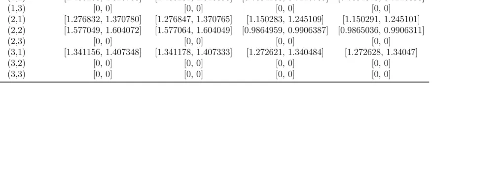
Table 4.3: Results of PE for the Michaelis-Menten Model

Initial Conditions Indeterminate set of c Feasible Set of c Indeterminate set of f Feasible Set off

(0,3) [0, 0] [0, 0] [0, 0] [0, 0]

(1,1) [1.101234, 1.269065] [1.101249, 1.269050] [0.7969512, 0.9675521] [0.7969665, 0.9675445] (1,2) [1.460266, 1.516708] [1.460281, 1.516693] [0.7094268, 0.7210769] [0.7094345, 0.7210693]

(1,3) [0, 0] [0, 0] [0, 0] [0, 0]

(2,1) [1.276832, 1.370780] [1.276847, 1.370765] [1.150283, 1.245109] [1.150291, 1.245101] (2,2) [1.577049, 1.604072] [1.577064, 1.604049] [0.9864959, 0.9906387] [0.9865036, 0.9906311]

(2,3) [0, 0] [0, 0] [0, 0] [0, 0]

(3,1) [1.341156, 1.407348] [1.341178, 1.407333] [1.272621, 1.340484] [1.272628, 1.34047]

(3,2) [0, 0] [0, 0] [0, 0] [0, 0]

(54)

4.3 Discussion

In both the examples of this chapter, we discarded the model which had empty feasible parameter sets for certain initial conditions and as a consequence, the other model is considered as the best model. However, our algorithm can also be applied for cases where the competing models have only non-empty feasible parameter sets. In such scenarios, the discrimination is done by evaluating the overall parameter bounds of each model.

As an example, we can go to back case study I and refer to tables 4.1 and 4.2. We can see the range of feasible parameter set corresponding to p6 is almost the same for both the models. However, a sufficient dissimilarity can be observed in the parameter range corresponding to p3. For model, the feasible parameter bound comes out to be 0.127525329 while for model 2, it is 0.64743042. Thus, p3 varies over a larger range in model 2 which implies amount of uncertainty associated with the parameters of model 2 is larger than that of model 1. Also, Figure 4.4 and Figure 4.5 show that the parameters of model 1 are more consistent than that of model 1. Thus, we can say that model 1 fits the data of the reference model better than model 2. In this chapter, we have shown how our algorithm can be applied to solve model discrimination problems. Using this approach we have captured the steady as well as the transient behavior of the given biological models. However, it is observed that during steady states, the models either bear very similar dynamics and thus can not be distinguished analytically, or give strange results due to cumulative error. As a result, we have preferred to analyze the models based on their transient phase dynamics. Also, the algorithm accumulates error, as time goes on. Thus, we have generated very few data points from the reference model and restricted the simulation time of the EMV algorithm to prevent the system from exploding.

(55)

(56)

Figure 4.5: Parameter Bound for Model 2

(57)

Chapter 5 Conclusion and Future Works

5.1 Conclusion

This thesis addressed the issue of model discrimination in biological systems. We pro-posed a solution method which is capable of providing promising results even with un-certain measurements and model parameters. A set-based approach has been developed where the uncertainty associated with the system is characterized by a continuous range of values and thus, gives more reliable results than methods assuming statistically defined noise or probabilistic uncertainty.

(58)

ap-plicable for invalidating models based on empty feasible parameter sets, but also for scenarios, where all the candidate models are having feasible parameter sets consistent with the generated data.

The key to our approach is in designing our algorithm in a set-based feasibility frame-work. This allows us to discard the regions which are not consistent with the experimental data and bounding the measurements in interval sets guarantees that no valid solution is lost.

Moreover, our algorithm is based on the improved parallelized parameter estimation algorithm [19] developed by Skylar et al. which efficiently uses multicore-chips of a computer to speed up the entire process. Based on the works presented in [20], this method is capable of producing reliable parameter estimates, even when uncertain and incomplete measurements are available.

Thus, we conclude that our proposed method is more effective than the other classical and contemporary model discrimination methods.

5.2 Limitations of the Proposed Method and Future

Scope

There is further scope of improvement in the work presented here.

• Computational burden resulting from the complexity of biological systems is still

(59)

model, this problem becomes more severe. Though, our algorithm is based on a parallelized parameter estimation algorithm, future developments can be made to run it on supercomputers using multi-processor GPUs. We can also reduce the computational burden by retaining larger feasible boxes, but that will result in inaccurate parameter estimates. An alternative solution may be to perform the sensitivity analysis of the model parameters and focus on estimating only those parameters upon which our system is sufficiently sensitive.

• Moreover, the EMV and SIVIA algorithms seem to be very model sensitive. Adding

error bounds on the state estimates result in negative lower state bounds for some model. This is not valid in practice as we are dealing with population models and chemical reaction models. Thus, our method works better in systems where relatively high number of data samples are available.

• One of the other drawbacks associated with set based approaches is the wrapping

effect. This can lead to very unreliable model predictions due to encasement of the predicted state output in an enclosure (e.g. interval boxes in our case) at each time step. Proper choice of enclosure shape is very crucial for this reason. Several methods have been proposed in the literature to resolve this issue. Incorporating those methods in our algorithm will lead to better results.

(60)

References

[1] Neumaier A. Interval Methods for Systems of Equations. Cambridge University Press, 1990.

[2] Joshua F. Apgar, Jared E. Toettcher, Drew Endy, Forest M. White, and Bruce Tidor. Stimulus Design for Model Selection and Validation in Cell Signaling. PLoS Computational Biology, 4(2), 2008.

[3] E. Balsa-Canto, A. A. Alonso, and J. R. Banga. Computational procedures for optimal experimental design in biological systems. IET Systems Biology, 2(4):163 – 172, 2008.

[4] L. Blackmore and B. Williams. Finite horizon control design for optimal model discrimination. Proc. IEEE Conf. Decision and Control, 2005.

[5] Stephen P. Brooks. Markov chain Monte Carlo method and its application. The Statistician, 47:69–100, 1998.

[6] Carolyn R Cho, Mark Labow, Mischa Reinhardt, Jan van Oostrum, and Manuel C Peitsch. The application of systems biology to drug discovery. Current Opinion in Chemical Biology, 10(4):294–302, 2006.

[7] Battogtokh D, Asch DK, Case ME, Arnold J, and Schottler HB. An ensemble method for identifying regulatory circuits with special reference to the qa gene cluster of Neurospora crassa. PNAS, 99:16904–16909, 2002.

(61)

[9] Casey FP, Baird D, Feng Q, Gutenkunst RN, Waterfall JJ, Myers CR, Brown KS, Cerione RA, and Sethna JP. Optimal experimental design in an epidermal growth factor receptor signalling and down-regulation model. IET Systems Biology, 1:190– 202, 2007.

[10] R Horn. Statistical methods for model discrimination. Applications to gating ki-netics and permeation of the acetylcholine receptor channel. Biophysical Journal, 51(2):255–263, 1987.

[11] Luc Jaulin and Eric Walter. Set Inversion via Interval Analysis for Nonlinear Bounded-error Estimation. Automatica, 29(4):1053–1064, 1993.

[12] Felsenstein K. Optimal Bayesian design for discrimination among rival models. Computational Statistics and Data Analysis, 14:427–436, 1992.

[13] Peter Kohl, Denis Noble, Raimond L. Winslow, and Peter J. Hunter. Computational modelling of biological systems: tools and visions. The Royal Society, 358:579–610, 2000.

[14] Brown KS and Sethna JP. Statistical mechanical approaches to models with many poorly known parameters. Physical Review E, 68(2), 2003.

[15] Gabriele Lillacci and Mustafa Khammash. Parameter Estimation and Model Selec-tion in ComputaSelec-tional Biology. PLoS Computational Biology, 6(3), 2010.

(62)

[17] Rodriguez-Fernandez M, Mendes P, and Banga JR. A hybrid approach for efficient and robust parameter estimation in biochemical pathways. iosystems, 83(2-3):248– 265, 2006.

[18] S. Marvel, M. de Luis Balaguer, and C. Williams. Interval Methods for Initial Value Problems in ODEs.

[19] Skylar W Marvel and Cranos M Williams. Set Membership Experimental Design for Biological Systems. Master’s thesis, North Carolina State University, 2011.

[20] Skylar W Marvel and Cranos M Williams. Set membership experimental design for biological systems. BMC Systems Biology, 6(21), 2012.

[21] Pedro Mendes and Douglas B. Kell. Non-linear optimization of biochemical path-ways: applications to metabolic engineering and parameter estimation. Bioinfor-matics, 14(10):869–883, 1998.

[22] Claas Michalik, Maxim Stuckert, and Wolfgang Marquardt. Optimal Experimental Design for Discriminating Numerous Model Candidates: The AWDC . Industrial and Engineering Chemistry Research, 49(2):913–919, 2009.

[23] Carmen G. Moles, Pedro Mendes, and Julio R. Banga. Parameter estimation in biochemical pathways: a comparison of global optimization methods. Genome Re-search, 13(11):2467–2474, 2003.

[24] Ramon E. Moore. Interval Analysis. Prentice-Hall, 1966.

(63)

[26] Nedialkov NS, Jackson KR, and Corliss G. Validated solutions of initial value prob-lems for ordinary differential equations. . Appl Math Comput, 105:21–68, 1999.

[27] Antonis Papachristodoulou and Hana El-Samad. Algorithms for Discriminating Be-tween Biochemical Reaction Network Models: Towards Systematic Experimental Design. In 2007 American Control Conference, 2007.

[28] Ricardo Paxson and Kristen Zannella. Systems Biology : Studying the Worlds Most Complex Dynamic Systems, 2007.

[29] Rihm R. Interval Methods for Initial Value Problems in ODEs. In Topics in vali-dated computations: Proceedings of the IMACS-GAMM international workshop on

validated computations, pages 173–208, 1994.

[30] T. Raissi, N. Ramdani, and Y. Candau. Set membership state and parameter estima-tion for systems described by nonlinear differential equaestima-tions. Automatica, 40:1771– 1777, 2004.

[31] Philipp Rumschinski, Steffen Borchers, Sandro Bosio, Robert Weismantel, and Rolf Findeisen. Set-base dynamical parameter estimation and model invalidation for biochemical reaction networks. BMC Systems Biology, 4(69), 2010.

[32] Schnell S, Chappell MJ, Evans ND, and Roussel MR. The mechanism distinguisha-bility problem in biochemical kinetics: The single-enzyme, single-substrate reaction as a case study. Compt rend-biol, 329:51–61, 2006.

(64)

[34] Dominik Skanda and Dirk Lebiedz. An optimal experimental design approach to model discrimination in dynamic biochemical systems. Bioinformatics, 26(7):939– 945, 2010.

[35] Steven H. Strogatz. Nonlinear Dynamics and Chaos. Perseus Books, 1994.

[36] Tina Toni and Michael P. H. Stumpf. Simulation-based model selection for dy-namical systems in systems and population biology. Bioinformatics, 26(1):104–110, 2010.

[37] Tina Toni, David Welch, Natalja Strelkowa, Andreas Ipsen, and Michael P. H. Stumpf. Approximate Bayesian computation scheme for parameter inference and model selection in dynamical systems. J. R. Soc. Interface, 6(31):187–202, 2009.

[38] Pablo Villoslada, Lawrence Steinman, and Sergio E. Baranzini. Systems Biology and Its Application to the Understanding of Neurological Diseases. Ann Neurol, 65(2):124–139, 2009.

Model Discrimination Using Bounded Error Estimation Approach

Abstract

Dedication

Biography

Acknowledgements

Table of Contents

List of Tables

List of Figures

Chapter 1

Introduction

1.1

Overview

1.2

Motivation

1.3

Thesis Contribution

1.3.1

Intellectual Merit

1.3.2

Broader Impacts

1.4

Thesis Organization

Chapter 2

Background

2.1

Overview

2.2

State of Art

2.3

Our Approach

2.4

Discussion

Chapter 3

Methodology

3.1

Overview

3.2

Biological Modeling

3.3

Problem Statement

3.4

Interval Analysis

3.4.1

Basic Tools

3.4.2

Inverse Image Evaluation (Set Inversion)

3.4.3

Direct Image Evaluation

3.5

Extended Mean Value Theorem and Set

Inver-sion via Interval Analysis

3.6

Parameter and State Estimation

3.7