DOI: 10.1534/genetics.107.077818
Analysis of Litter Size and Average Litter Weight in Pigs
Using a Recursive Model
Luis Varona,*
,1Daniel Sorensen
†and Robin Thompson
‡,§*Gene´tica i Millora Animal, IRTA, 25198 Lleida, Spain,†Department of Genetics and Biotechnology, Faculty of Agricultural Sciences, University of Aarhus, DK-8830 Tjele, Denmark,‡School of Mathematical Sciences,
University of London, London E1 4NS, United Kingdom and§Centre for Mathematical and Computational Biology, Department of Biomathematics and Bioinformatics,
Rothamsted Research, Harpenden AL5 2JQ, United Kingdom
Manuscript received June 18, 2007 Accepted for publication August 16, 2007
ABSTRACT
An analysis of litter size and average piglet weight at birth in Landrace and Yorkshire using a standard two-trait mixed model (SMM) and a recursive mixed model (RMM) is presented. The RMM establishes a one-way link from litter size to average piglet weight. It is shown that there is a one-to-one correspondence between the parameters of SMM and RMM and that they generate equivalent likelihoods. As param-eterized in this work, the RMM tests for the presence of a recursive relationship between additive genetic values, permanent environmental effects, and specific environmental effects of litter size, on average piglet weight. The equivalent standard mixed model tests whether or not the covariance matrices of the random effects have a diagonal structure. In Landrace, posterior predictive model checking supports a model without any form of recursion or, alternatively, a SMM with diagonal covariance matrices of the three random effects. In Yorkshire, the same criterion favors a model with recursion at the level of specific environmental effects only, or, in terms of the SMM, the association between traits is shown to be exclusively due to an environmental (negative) correlation. It is argued that the choice between a SMM or a RMM should be guided by the availability of software, by ease of interpretation, or by the need to test a particular theory or hypothesis that may best be formulated under one parameterization and not the other.
M
IXED linear models (Henderson 1984) arebroadly used to predict breeding values and to estimate variance components for traits of interest in livestock and plant breeding and play an important role in evolutionary and theoretical quantitative genetics
(Lande 1979; Cheverud1984; Walsh 2003). In
ge-netic improvement programs, the objective of selection includes typically several correlated traits. The classical approach for a multiple-trait analysis is to use models posing that the nature of the correlation between re-sponse variables (phenotypes) is due to linear associ-ations between unobservables, such as additive genetic values or nongenetic sources, like permanent or tem-porary environmental effects.
Structural equation models represent an extension of the standard linear model to account for links (feedback and/or recursiveness) involving either the phenotypes directly or latent variables; they are well established in econometrics and sociology (Goldberger1972; Jo¨ reskog
1973; Duncan1975). These models were discussed in the
early genetics literature by Wright(1921) but this work has
not received much attention in quantitative genetics. Re-cently, Xionget al. (2004) proposed the use of structural
equation models for modeling and identifying genetic networks. In a quantitative genetics context, Gianolaand
Sorensen(2004) studied the consequences of the existence
of simultaneous and recursive relationships between pheno-types on genetic parameters and presented statistical meth-ods for inference. A recent application to study the relationship between somatic cell score and milk yield in goats is in de losCamposet al.(2006). Here we are
con-cerned with an illustration of the implementation of struc-tural equation models for the analysis of litter size and average litter weight in two breeds of Danish pigs.
Litter size is an important trait in pig genetic
im-provement programs (Rothschildand Bidanel1998)
and there is now convincing evidence that it has re-sponded successfully to selection (i.e., Sorensenet al.
2000; Nogueraet al.2002). Several studies have also
re-ported negative associations between litter size and
in-dividual birth weight (Kerrand Cameron1995; Roehe
1999; Sorensen et al.2000). Further, Sorensen et al.
(2000) report an increase in the proportion of piglets born dead at higher litter size values.
Litter size is basically determined by ovulation rate
and embryo mortality (Blascoet al.1995); these
pro-cesses take place mainly at the early stages of ges-tation. Piglet weight at birth is mostly determined by growth in late gestation. One could then postulate a
1Corresponding author: Genetica I Millora Animal, IRTA, Av. Rovira
Roure 177, 25198 Lleida, Spain. E-mail: [email protected]
one-way causal path establishing an effect of litter size on piglet weight at birth. This specification defines a recursive two-trait system. On the other hand, simul-taneity occurs when trait 1 affects trait 2 and vice versa. The objective of this study is, first, to show that re-cursive models can be interpreted as alternative pa-rameterizations of standard linear models. We discuss identifiability of dispersion parameters, a topic that is intimately connected to the possibility of drawing infer-ences from the various parametric forms of a given model. Second, we address the statistical problems involved in deciding whether the association between traits is me-diated by additive genetic and/or environmental cova-riances or via recursion only. The results are illustrated using data on litter size and average litter weight in pigs.
MATERIALS AND METHODS
Data: Data from two breeds were analyzed: Landrace and Yorkshire. The traits analyzed were total number born per litter and average litter weight at birth (referred to as litter size and average piglet weight, hereinafter). The Landrace data set included 5178 litter size records and a pedigree file of 8800 individuals. The raw means for litter size and average piglet weight were 14.23 piglets and 1.36 kg., respectively, with standard deviations 3.62 piglets and 0.35 kg. The Yorkshire data set consisted of 3938 litter size records and a pedigree file of 7143 individuals. The raw means for litter size and average piglet weight were 13.01 piglets and 1.30 kg., respectively, with standard deviations 3.40 piglets and 0.22 kg. The raw correlations between traits were 0.01 in Landrace and0.43 in Yorkshire. Piglet weight at birth is strongly genetically determined by maternal effects (Grandinsonet al.2002), and, as a
conse-quence, average piglet weight (as well as litter size) was con-sidered a trait of the sow.
Models and likelihoods: A description is provided of a standard mixed model (SMM) and a recursive mixed model (RMM). The SMM postulates the following linear structures foryLij(subscriptLrepresents litter size) andyWij(subscriptW
represents average piglet weight) of thejth pair of records from femalei,
yLij¼xLij9 bL1uLi1pLi1eLij; ð1aÞ
yWij¼xWij9 bW1uWi1pWi1eWij; ð1bÞ
where xkij9 (k ¼ L, W) is the appropriate row of a known incidence matrix,bkis a vector containing effects of herd years, seasons, and parity number,ukiis an additive genetic effect of
individual i, pki is a permanent environmental effect of
individuali, andekijis a residual effect (the lengths of the vectors of additive genetic effects and data are different, but to simplify notation, it is assumed throughout that after an
ap-propriate relabeling, a common subindexican be used for
y,u, andp).
The following distributions were assigned to the location parameters:
ðbL;bWÞ Nðð0;0Þ;I105Þ; ðuLi;uWijGÞ Nðð0;0Þ;GÞ;
ðpLi;pWijPÞ Nðð0;0Þ;PÞ; ðeLij;eWijjRijÞ Nðð0;0Þ;RijÞ: ð2Þ
Above,Iis the identity matrix (of appropriate order),
G¼ s
2
uL suLuW
suLuW s
2
uW
" #
; ð3Þ
and
P¼ s
2
pL spLpW
spLpW s
2
pW
" #
: ð4Þ
The termss2
xmandsxLxW (x¼u,p;m¼L,W) in (3) and (4) are
variance and covariance components associated with the distribution of additive genetic effects (x¼u) and permanent environmental effects (x¼p) for litter size and for individual piglet weight.
A possible approach to modeling the residual termRijis as follows. Assume that the residual terms for individual piglet weight at birth that contribute to a given average piglet weight are conditionally normally and independently distributed, given litter size, with residual variances2
eW 1r 2 eLeW
, where
s2
eW is the residual component of variance of individual piglet
weight at birth andreLeW is the residual correlation between litter size and individual piglet weight at birth. Also assume that the residual terms for litter size are normally distributed with variances2
eL. Then the marginal (with respect to litter
size) residual covariance between two individual piglet weight at birth records isr2
eLeWs 2
eW and the residual covariance matrix
is equal to
Rij ¼
s2e
L reLeWseLseW
re
LeWseLseW
s2
eW
nij
ð11ðnij1Þr2eLeWÞ
2 6 4
3 7
5: ð5Þ
In (5), the off-diagonal termreLeWseLseW ¼seLeW, andnijis
the known number of records contributing to the average piglet weight of femaleiin parityj. There are three identifi-able parameters in (5). This residual dispersion matrix can also be written as
Rij¼
s2
eL beLeWs
2
eL
be
LeWs
2
eL
s2
eW
nij
1nij1 nij
b2
eLeWs
2
eL
2 6 4
3 7
5; ð6Þ
wherebeLeW ¼seLeW=s2eL is the residual regression of
individ-ual piglet weight at birth on litter size. MatrixRijis positive definite since s2
eLs 2 eW=nij
ð11ðnij1Þr2Þ.r2 eLeWs
2 eLs
2 eW. The
residual covariance matrix (5) fornij¼1 is denoted byR. The heritabilities for the two traits are
h2L¼
s2
uL
s2
uL1s
2
pL1s
2
eL
;
h2W ¼
s2
uW
s2u
W1s
2
pW1ðs
2
eW=nijÞð11ðnij1Þr
2
eLeWÞ
; ð7Þ
and the coefficients of correlation are
rxLxW ¼ sxLxW
sxLsxW
; x¼u;p;e: ð8Þ
Writingyij¼(yLij,yWij)9, Equations 1 can be expressed as
yij¼Xijb1ui1pi1eij; ð9Þ
Xij¼
xLij9 0
0 xWij9
; b¼ ðbL9;bW9Þ9; ui¼ ðuLi;uWiÞ9;
pi¼ ðpLi;pWiÞ9; eij¼ ðeLij;eWijÞ9:
It follows that the sampling model for yij is the Gaussian
process
yijjb;ui;pi;Rij NðXijb1ui1pi;RijÞ ð10Þ
and the contribution to the likelihood byyijis
yijjb;G;P;Rij NðXijb;G1P1RijÞ: ð11Þ
The RMM assumes the following linear relationships be-tween thejth pair of records from individualiand location parameters,
yLij¼xLij9 bL1uLi1pLi1eLij; ð12aÞ
yWij¼lðyLijxLij9 bLÞ1xWij9 bW1uWi* 1pWi* 1eWij* ; ð12bÞ
wherelis the recursive parameter. The first term in the right-hand side of (12b) indicates that, according to the model, average piglet weight is linearly related to the deviation of litter size from its group mean, and the strength of this relationship is measured byl. On the other hand, Gianola
and Sorensen(2004) postulate recursiveness or simultaneity
between traits involving the observed phenotypes, rather than the unobserved deviations. We return to this point in
thediscussion.
The system defined by (12) can be retrieved subtracting the mean on both sides of (9) and multiplying byL, to get
LðyijXijbÞ ¼Lui1Lpi1Leij
¼u*i1p*i1e*ij: ð13Þ
The reduced form of (13) is
yij¼Xijb1L1u*i1L
1p*
i1L
1e*
ij; ð14Þ
which is the same as (9), where
L1¼ 1 0
l 1
1
¼ 1 0
l 1
;
and
z*
i ¼
zLi*
z*
Wi
¼ zLi
zWilzLi
; z*
i ¼u*i;p*i;e*ij; z¼u;p;ej:
It follows from the Gaussian form of the distributions (2) that
u*
ijG*Nðð0;0Þ;G*Þ; p*ijP*Nðð0;0Þ;P*Þ;
e*ijjR*ijNðð0;0Þ;R*ijÞ; ð15Þ
where
G*¼LGL9;
P*¼LPL9; ð16Þ
R*ij ¼LRijL9:
Therefore the sampling model foryijunder the RMM is the
Gaussian process
yijjb;u*i;p*i;R
*
ij NðXijb1L1u*i1L
1p*
i;R
*
ijÞ; ð17Þ
and the contribution to the likelihood byyijis
yijjb;G*;P*;R*ij;lNðXijb;L1ðG*1P*1R*ijÞðL
1Þ9Þ:
ð18Þ
Iflwere known this is the same likelihood as (11) due to the one-to-one relationship
L1ðG*1P*1R*
ijÞðL
1Þ9¼G1P1R
ij: ð19Þ
However, with unknownl, the left-hand side of (19) contains 10 parameters and the right-hand side 9. There are thus an infinite number of matrices involving the left-hand side of (19) that satisfy the equality, for any givenG1P1Rij. In other words, disregarding identifiability at the level of the mean for both models, the RMM as defined above generates an un-identifiable likelihood.
Likelihood identification under the SMM and the RMM:
The subject of identifiability of the SMM and the RMM at the level of the mean is well known (e.g., Searle1971) and is not
discussed. In likelihood (11) of the SMM there are nine identifiable dispersion parameters associated withG,P, and
Rij. This model with nondiagonal covariance matrices foru,p, andeis labeled SMMupe.
The RMM has an extra parameter, and a constraint needs to be introduced to achieve identification. One possible con-straint is to assume that the phenotypic covariance on the recursive scale is zero. That is, denoting the mean ofyLbymL,
CovðyL;yW lðyLmLÞÞ
¼CovðuL;u*WÞ1CovðpL;pW*Þ1CovðeL;eW*Þ
¼CovðuL;uWluLÞ1CovðpL;pW lpLÞ
1CovðeL;eWleLÞ
¼suLuW1spLpW1seLeW lðs
2
uL1s
2
pL1s
2
eLÞ ¼0: ð20Þ
This places the following interpretation onl,
l¼suLuW1spLpW1seLeW
s2
uL1s
2
pL1s
2
eL
; ð21Þ
the phenotypic regression of average litter weight on litter size. Expanding (19) it is easy to show that the constraint (20) guarantees a one-to-one relationship between the dispersion
parameters of the RMM and those of the SMMupe and the
likelihoods become equivalent. In this setting the RMM subject to the chosen constraint and the unconstraint SMMupe
are two different identifiable parameterizations of the same likelihood model.
From the point of view of a likelihood analysis, inferences on the recursive scale can be obtained by fitting the SMMupe
and transforming the estimated parameters appropriately, and vice versa. However, it is not statistically meaningful to ask whether the data have been generated by the SMMupeor by the
recursive process described by the RMM subject to constraint (20), since both specifications lead to the same likelihood.
Generating an identifiable likelihood model to address the nature of the relationship between traits:Here we present a statistically meaningful way to address the question whether the data have been generated by a recursive mechanism.
˜ G¼ s˜
2
uL 0
0 s˜2
uW
" #
; ð22Þ
˜ P¼ s˜
2
PL 0
0 s˜2
PW
" #
; ð23Þ
and
˜ Rij ¼
˜
s2
eL 0
0 s˜
2 ew nij 2 6 4 3 7
5: ð24Þ
The contribution to the likelihood by the pair of recordsyijis
yijjb;G;˜ P;˜ R˜ijNðXijb;ðG˜1P˜1R˜ijÞÞ: ð25Þ
There are six dispersion parameters associated with this model (the covariance matrices ofu,p, andehave 0 off-diagonal ele-ments), which is labeled SMM0.
The RMM that is developed here postulates that the rela-tionship between data and location parameters is now
yij¼Xijb1Luui1Lppi1Leeij
¼Xijb1u
d
i1p
d
i1e
d
ij;
ð26Þ
whereui,pi, andeijare the same stochastic variables as in the SMM0with covariance matrices (22), (23), and (24), and with
Lu¼ l1 0
u 1
;
ud
i9¼ ðu
d
Li;u
d
WiÞ ¼ ðuLi;uWi1luuLiÞ; ð27Þ
and similarly forLp,Le,p
d
i, ande
d
ij. Note that theL’s in (26)
have the same structure as theL1in (14). Contrary to the generation of recursion in (13), the recursive model defined by (26) is not obtained by a linear transformation of the SMM and the two models lead to different marginal (with respect to random effects) distributions of the data. The linear structure specified by (26) and (27) has an interesting property: the components of average litter weightðzWi1lxzLiÞ,z¼u,p,e,
have a termzWi independent of litter size and a component
lxzLi dependent on litter size.
The sampling model foryijis
yijjb;ud
i;p
d
i;R
d
ij NðXijb1u
d
i1p
d
i;R
d
ijÞ; ð28Þ
and the contribution to the likelihood fromyijis
yijjb;Gd
;Pd
;Rd
ij NðXijb;G
d 1Pd
1Rd
ijÞ; ð29Þ
where Gd
¼LuG˜Lu9, P
d
¼LpP˜Lp9, and R
d
ij ¼LeRij˜ Le9. This
form of recursive model is labeled RMMupe. There are nine
identifiable parameters in the dispersion matrix of this likeli-hood and whenlu¼lp¼le¼0 (or whenLu¼Lp¼Le¼I),
likelihood (29) is equal to (25). A comparison between
RMMupeand RMM with lu¼ lp¼le¼ 0, which is labeled
RMM0, is to jointly test whether or not there is recursion at the level of the unobservable additive genetic values, permanent environmental and environmental effects. Alternatively, since likelihoods (29) and (11) are equivalent½it is easy to see that, for example, ˜s2
uL ¼s 2 ud
L ¼s 2 uLand ˜s
2
uW ¼ 1r 2 uLuW
s2 uWthe
comparison can be interpreted as testing whether or not the covariance matrices of the random effects of the SMMupehave
a diagonal structure. Indeed, note that
Gd
¼ s
2
ud
L su
d
Lu
d
W
sud
Lu d W s 2 ud W " #
¼ s˜
2
uL lus˜
2
uL
lus˜2uL s˜
2
uw1l
2
us˜2uL
" #
; ð30Þ
Pd
¼ s
2
pd
L sp
d
Lp
d
W
spd
Lp d W s 2 pd W " #
¼ s˜
2
pL lps˜
2
pL
lps˜2pL s˜
2
pw1l
2
ps˜2pL
" #
; ð31Þ
Rd
ij¼
˜
s2
eL les˜
2
eL
les˜2eL
˜
s2
ew
nij
1l2es˜2e
L 2 6 4 3 7
5: ð32Þ
The bottom diagonal element in (32) is very similar to the corresponding element in (6). However, when the trait is not average (that is, whennij¼1), the second term in the bottom diagonal element of (6) vanishes. Since, for example,
suLuW ¼buLuWs2uL, by inspection of (30), (31), and (32) with
(3), (4), and (6) it is obvious that theb’s under the SMM are identical to thel’s in the RMM.
We also need
Rd
¼ s
2
ed
L se
d
Le
d
W
sed
Le d W s 2 ed W " #
¼ s˜
2
eL les˜
2
eL
les˜2eL s˜
2
ew1l
2
es˜
2
eL
" #
; ð33Þ
which is matrixRd
ijfornij¼1. Whenlu¼lp¼le¼0, the above
covariance matrices become equal to (22), (23), and (24). Under the RMMupe, the heritability of average litter weight
fornij¼nTfor alli,jis defined as
h2Wd¼
s2ud
W
s2
ud
W1s
2
pd
W1s
2
ed
W
: ð34Þ
Prior and posterior distributions:For the RMMupe, the joint
prior distribution of all parameters is assumed to admit the factorization
pðb;ud
;pd
;Gd
;Pd
;Rd Þ ¼pðbÞpðud
jGd Þpðpd
jPd ÞpðGd
ÞpðPd ÞpðRd
Þ; ð35Þ
whereudis the vector that contains the pairsðuLi;uWiÞfor all individuals in the pedigree, andpdis the vector that contains all permanent environmental effectsðpLi;pWiÞof females with
records. The vector b is allocated an improper uniform
distribution and vectorsudandpdare assumed to be normally distributed
ud jGd
;ANð0;A5G
d Þ;
whereAis the known additive genetic relationship matrix, and
pd jPd
Nð0;I5P
d Þ:
The 2 3 2 matrices Gd
, Pd , and Rd
follow inverse Wishart distributions
Gd jGd
0; vG IWðG
d
0;vGÞ;
Pd jPd
0; vpIWðP
d
0;vPÞ;
Rd jRd
0; vR IWðR
d
where the hyperpriorsGd 0,P
d 0, andR
d
0are known matrices of
dimension 232 and thev’s are known degrees of freedom.
The conditional density for the total datay¼ fyijgis equal to
pðyjb;ud
;pd
;Sd
Þ ¼Y
i;j
pðyijjb;ud
i;p
d
i;R
d
ijÞ; ð36Þ
whereSd
is a block diagonal with blocksRd
ij associated with
each pair of recordsyij.
The posterior distribution of the RMMupe, up to a
propor-tionality constant, is obtained by multiplication of the joint prior (35) by (36), giving
pðb;ud
;pd
;Gd
;Pd
;Rd jyÞ
}pðyjb;ud
;pd
;Sd Þpðud
jGd Þpðpd
jPd ÞpðGd
Þ
3pðPd ÞpðRd
Þ; ð37Þ
which is also the posterior distribution of SMMupe, the
standard two-trait mixed model with nondiagonal covariance matrices associated with all the random effects. Inferences based on RMMupecan be drawn from the posterior distribution
(37) and the recursive parameters can easily be constructed from (30), (31), and (33),
lu¼
sud
Lu
d
W
˜
s2u
L
; ð38Þ
lp¼
spd
Lp
d
W
˜
s2
aL
; ð39Þ
and
le¼
sed
Le
d
W
˜
s2e
L
: ð40Þ
A variety of submodels can be generated either by assuming some or all of thel’s equal or by setting some of them equal to zero.
Implementation:If the number of piglets born was the same for all litters,nT, say, thenS
d
¼I5R
d
nT, whereR
d
nTdenotes the
residual covariance matrix (32) withnijreplaced bynT. In this case, the structure of pðyjb;ud
;pd
;Sd
Þ in (37) simplifies
considerably. To take advantage of this simplification in the computations one can augment the piglet weight data with the so-called missing single recordsymis
W , so thatnij¼nTfor allij,
where nT is the largest number of records contributing to
average piglet weight in the data set. This technique is known
as data augmentation (Tanner and Wong 1987) and the
general idea is as follows. Given observed datayand a model indexed by parametersu, the posterior distributionpðujyÞis proportional topðyjuÞpðuÞ. When the model is fitted using MCMC, drawing samples from this posterior distribution may be computationally demanding. However, it may be easy to draw samples from
pðujy;ymisÞ}pðy;ymisjuÞpðuÞ
}pðymis;ujyÞ;
whereymisstands for the missing data. The strategy requires generating ymis from ½ymisju;y. In the present case, ymis
W is
generated from
NðEðymisW jyW;yL;uÞ;VarðymisW jyW;yL;uÞÞ;
whereuis the vector of all parameters indexing the model.
After a little experimentation, a length of the Gibbs chain equal to 1 million was chosen. In Tables 1 and 2 we report Monte Carlo standard errors of estimates of various posterior means to give an idea of the accuracy of the Monte Carlo computations.
Model testing:Checking for systematic differences between a given model and the observed data discloses the quality of fit of the posed model. An attractive way to study the fit of a model is to use posterior predictive model checking (Gelmanet al.
1996, 2004). The approach is simple to implement, is flexible, and provides a graphical exploration of residual-type diag-nostics. The key feature is the construction of the so-called discrepancy measures that describe particular putative fea-tures of the data that the model may fail to account for. To be more specific, consider testing for the presence of recursion at the level of permanent environmental effects. Absence or presence of recursion at the level of additive genetic effects or residuals is studied in a similar way. Let (yLij,yWij),i¼1, 2,. . ., denote observed data and for parityj¼1, define the discrep-ancy measure
bp¼
P
iðyWi1PxWi9 1bWÞðpLipLÞ iðpLipLÞ2
; ð41Þ
the change of average piglet weight per unit change of permanent environmental effect associated with litter size. In (41), the sum is over all females with first parity records, and
pLis the averagepLiacross females. If the observed data had
been generated under RMM0one would expect a value ofbpin the vicinity of zero. If parameters were known, one could compare the observed value ofbpto its sampling distribution, with a significant difference indicating model failure with respect to the discrepancy measure. This is equivalent to simulating data ðyrepLi1;y
rep
Wi1Þ,i¼1, 2,. . ., under the RMM0, if parameters were known, computingbrepp in each replicate, and
deciding whether the observed value ofbpis an atypical value in the distribution ofbprep. Specifically and in the current context,
one is testing whether the null model RMM0is failing to account for a recursive mechanism present in the observed data.
Since parameters are not known, we use the idea of pos-terior predictive model checking (Gelmanet al.1996, 2004)
and consider the posterior predictive distribution ofbpbprep.
This distribution reflects uncertainty about the parameters that enter in the discrepancy measure (41) as well as sampling variation. Note that the parameters are inferred from the ‘‘null
model’’ RMM0that assumes absence of recursion. The
pres-ence of recursion, not accounted for by model RMM0would
result in a distribution ofbpbprepshifted from zero. This can
also be construed as a test for a nonzero covariance between permanent environmental effects affecting litter size and those affecting average piglet weight. The exploration of recursion at the level of additive genetic effects and of residuals involves constructingbubrep
u andbeb rep
e along the same lines.
Often the diagnostic results of posterior predictive model checking are apparent visually, as is the case in this work. Other times it can be useful to compute a posterior predictiveP-value to see whether the results could have arisen by chance under the null model (Gelmanet al.1996, 2004). These can be very
easily computed from the MCMC output.
RESULTS
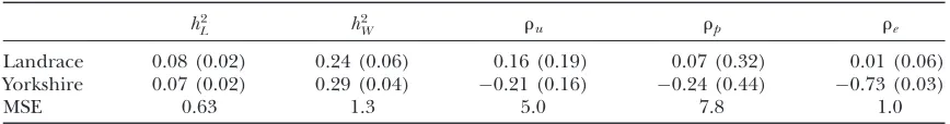
The familiar parameterization in a two-trait
mixed-model analysis is based on mixed-model SMMupe. We therefore
based on the SMMupefor Landrace and Yorkshire. Due
to the symmetry of all the posterior distributions re-ferred to below, standard deviations rather than poste-rior intervals are reported. The numbers in the table indicate that there is a striking difference between the breeds, especially for the size and the sign of the corre-lation coefficients. For Landrace, a value in the vicinity of zero for all three correlation coefficients is in an area of high probability mass. For Yorkshire, only for the en-vironmental correlation is the value of zero excluded in the 95% posterior interval.
Table 2 shows Monte Carlo estimates of posterior means and standard deviations for chosen parameters
based on the RMMupe parameterization for Landrace
and Yorkshire. There is a one-to-one relation between
the parameters of the RMMupeand those of the SMMupe.
The conclusions based on the recursive parameters are the same as those based on the correlation coefficients from Table 1.
Figures 1 and 2 show the posterior predictive distri-bution of discrepanciesbuburep,bpb
rep
p , andbeberep
for Landrace and Yorkshire generated under RMM0.
For Landrace, the Monte Carlo estimates of the poste-rior means (posteposte-rior standard deviations) for the three discrepancy measures are 0.067 (0.280), 0.019 (0.020),
and0.000 (0.003), reflecting lack of recursion at all
levels. There is therefore lack of evidence suggesting that there is conflict between the data and the null
model RMM0, with respect to the feature described by
the discrepancy measure. For Yorkshire, the
corre-sponding numbers are 0.057 (0.052), 0.030
(0.019), and 0.034 (0.002), supporting recursion at
the level of the residual term only, a feature of the data that the null model fails to account for.
DISCUSSION
In a recent article, Gianola and Sorensen (2004)
discussed the use of simultaneous equation models to analyze and interpret systems of traits that may be subject to feedback and recursive relationships. Here we report an application of a recursive mixed model for the analysis of litter size and average piglet weight in two breeds of Danish pigs. The recursive relationship defined by model (12) establishes that average piglet weight is linearly related to the deviation of litter size from its group mean.
The traditional specification, like that in Gianolaand
Sorensen(2004), postulates that average piglet weight is
linearly related to litter size, rather than to its deviation from the mean. The system defined by (12) is free of some identifiability problems at the level of parameters entering the mean that are common to both traits. It seems also appealing that deviations from a midvalue, rather then absolute values, exert an influence on average pig-let weight. Ultimately, these are two different models and a way of discerning between them is by computing their posterior probabilities, in the light of the data. This was not studied in the present work.
The structure of the residual dispersion matrix (5) has three parameters and was arrived at assuming that
TABLE 1
Monte Carlo estimates of posterior means of chosen parameters (posterior standard deviations in parentheses) based on SMMupe
h2
L h
2
W ru rp re
Landrace 0.08 (0.02) 0.24 (0.06) 0.16 (0.19) 0.07 (0.32) 0.01 (0.06)
Yorkshire 0.07 (0.02) 0.29 (0.04) 0.21 (0.16) 0.24 (0.44) 0.73 (0.03)
MSE 0.63 1.3 5.0 7.8 1.0
h2, heritability with subscriptsL(litter size) andW(average piglet weight) forn
T¼25 individuals;r, corre-lations with subscriptsu,p, andeinvolving additive genetic, permanent, and environmental effects; MSE, Monte Carlo standard error3104.
TABLE 2
Monte Carlo estimates of posterior means of chosen parameters (posterior standard deviations in parentheses) based on RMMupe
h2
L h
2
Wd lu lp le
Landrace 0.08 (0.02) 0.24 (0.06) 0.022 (0.026) 0.050 (0.189) 0.000 (0.003)
Yorkshire 0.07 (0.02) 0.22 (0.03) 0.028 (0.022) 0.028 (0.067) 0.034 (0.003)
MSE 0.60 1.3 5.6 9.5 1.7
h2, heritability with subscriptsL(litter size) andWd
the covariance between residuals for single weight
measurements is r2
eLeWs
2
eW. This leads to conditionally
independent residuals, given litter size. A more general model would assume that the above covariance is
re
WeWs
2
eW, wherereWeW is the residual correlation between
single weight measurements. Then residuals are no longer conditionally independent, given litter size. The resulting residual covariance matrix between litter size
Figure1.—(Landrace) Estimates of posterior distributions
(under RMM0) of discrepanciesbuburep(left),bpb rep
p
(cen-ter), andbebrep
e (right).
Figure2.—(Yorkshire) Estimates of posterior distributions
(under RMM0) of discrepanciesbubrepu (left),bpb rep
p
(cen-ter), andbebrep
and average litter weight has four identifiable parame-ters and retrieves (5) whenre
WeW ¼r
2
eLeW. This model has
also its recursive parameterization counterpart. The saturated recursive model used in this work has nine identifiable dispersion parameters. A more parsi-monious alternative with seven parameters postulates that the three recursive parameters lu, lp, and le are
equal. In general, the recursive parameterization can be an attractive approach to arrive at parsimonious models, especially in analyses involving many traits.
Special attention has been given here to identifi-ability at the level of the likelihood, despite the fact that inferences were based on posterior distributions. In principle, a Bayesian analysis with a nonidentifiable likelihood is possible if proper prior distributions are
specified for all the parameters (Bernardoand Smith
1994). In fact, depending on the prior distributions, a Bayesian analysis with a nonidentifiable likelihood may result in Bayesian learning, in the sense that the pos-terior and prior distributions of the nonidentified
pa-rameters are different (see, for example, Sorensenand
Gianola 2002, p. 543). However, an MCMC
imple-mentation of a Bayesian model with ‘‘barely’’ identified parameters can lead to poor inferences due to extremely slow convergence and very short effective chain lengths. Achieving identifiability of parameters at the level of the likelihood will always lead to Bayesian learning and in general to better behavior of the MCMC algorithm. How-ever, there may be situations where the constraints needed for identifiability may restrict inferences, and an un-constrained model using a careful prior specification could be considered instead.
The analyses of Yorkshire and Landrace data lead to markedly different inferences; we are not disturbed by this result. The breeds are distinct in various behavioral, physiological, and anatomical traits, as well as in out-ward appearance. From a breeding point of view, in Landrace, changes in litter size should not lead to associated changes in average litter weight. In Yorkshire, a change in environmental deviation of litter size of 1 unit (for example, due to culling) should result in a tem-porary reduction of average piglet weight of 36 g. In neither breed should successful selection for litter size have a direct effect on average piglet weight.
There is a rich literature dealing with various trans-formations of the data or reparameterizations that can lead to computationally more tractable analyses of the
multivariate linear model (for example, Meyer1987;
Jensen and Mao 1988; Quaas 1988; Ducrocq and
Besbes1993; Groeneveld1994; Gelfandet al. 1995;
Thompsonet al. 1995; Ducrocq and Chapuis 1997).
While the recursive model can be viewed in this frame-work, the focus of the present work is that a recursive model whose likelihood is identifiable is an alternative parameterization of a standard mixed model. The two models provide different interpretations of the results, but are statistically equivalent. There is a one-to-one
relationship between the parameters entering the likeli-hood in both models. This applies also in principle to simultaneous equation models, which in general re-quire a larger number of constraints to achieve identifi-ability. However, it may not always be easy to define the equivalent standard model, say, to a model involving complex simultaneous and recursive relationships among many traits. Ultimately, the choice of parameterization should be guided by the availability of software (in sim-ple situations like in the present work), by ease of in-terpretation, or by the need to test a particular theory or hypothesis. The mathematical formulation of such a hy-pothesis may be more naturally accomplished using one parameterization and not the other.
We are grateful to Gustavo de los Campos and Daniel Gianola for discussions and comments on an earlier version of this manuscript.
LITERATURE CITED
Bernardo, J. M., and A. F. M. Smith, 1994 Bayesian Theory.Wiley,
New York.
Blasco, A., J. P. Bidaneland C. Haley, 1995 Genetics and neonatal
survival, pp. 17–38 inThe Neonatal Pig. Development and Survival, edited by M. A. Varley. CAB International, Wallingford, Oxon,
UK.
Cheverud, J. M., 1984 Quantitative genetics and developmental
constraints on evolution by selection. J. Theor. Biol.110:155– 171.
de los Campos, G., D. Gianola, P. Boettcher and P. Moroni,
2006 A structural equation model for describing relationships between somatic cell score and milk yield in dairy goats. J. Anim. Sci.84:2934–2941.
Ducrocq, V., and B. Besbes, 1993 Solution of multiple trait animal
models with missing data on some traits. J. Anim. Breed. Genet. 110:81–92.
Ducrocq, V., and H. Chapuis, 1997 Generalising the use of the
ca-nonical transformation for the solution of multivariate mixed model equations. Genet. Sel. Evol.29:205–224.
Duncan, O. D., 1975 Introduction to Structural Equation Models.
Aca-demic Press, San Diego.
Gelfand, A. E., S. K. Sahuand B. P. Carlin, 1995 Efficient
param-eterization for normal linear mixed models. Biometrika82:479– 488.
Gelman, A., X. L. Mengand H. Stern, 1996 Posterior predictive
assessment of model fitness via realized discrepancies (with dis-cussion). Stat. Sin.6:733–807.
Gelman, A., J. B. Carlin, H. S. Sternand D. B. Rubin, 2004 Bayesian Data Analysis.Chapman & Hall, London/New York.
Gianola, D., and D. Sorensen, 2004 Quantitative genetic models
describing simultaneous and recursive relationships between phenotypes. Genetics167:1407–1424.
Goldberger, A. S., 1972 Structural equation methods in the social
sciences. Econometrica40:979–1001.
Grandinson, K., M. S. Lund, L. Rydhmer and E. Strandberg,
2002 Genetic parameters for piglet mortality traits crushing, stillbirth and total mortality, and their relation to birth weight. Acta Agric. Scand. Ser. A. Anim. Sci.52:167–173.
Groeneveld, E., 1994 A reparameterization to improve numerical
optimization in multivariate REML (co)variance component es-timation. Genet. Sel. Evol.26:537–545.
Henderson, C. R., 1984 Applications of Linear Models in Animal Breed-ing.University of Guelph, Guelph, ON, Canada.
Jensen, J., and I. L. Mao, 1988 Transformation algorithms in
anal-ysis of single trait and of multiple trait models with equal design matrices and one random factor per trait: a review. J. Anim. Sci. 26:2750–2761.
Jo¨ reskog, K. G., 1973 A general method for estimating a linear
structural equation system, pp. 85–112 inStructural Equation Mod-els in the Social Sciences, edited by A. S. Goldbergerand O. D.
Kerr, J. C., and N. D. Cameron, 1995 Reproductive performance of
pigs selected for components of efficient lean growth. Anim. Sci. 60:281–290.
Lande, R., 1979 Quantitative genetic analysis of multivariate
evolu-tion, applied to brain:body allometry. Evolution33:402–416. Meyer, K., 1987 A note on the use of an equivalent model to
ac-count for relationships between animals in estimating variance components. J. Anim. Breed. Genet.104:163–168.
Noguera, J. L., L. Varona, D. Babotand J. Estany, 2002
Multi-variate analysis of litter size for multiple parities with production traits in pigs: II. Response to selection for litter size and corre-lated responses to production traits. J. Anim. Sci.80:2548–2555. Quaas, R. L., 1988 Transformed mixed model equations: a
recur-sive algorithm to eliminateA1. J. Dairy Sci.72:1937–1941.
Roehe, R., 1999 Genetic determination of individual birthweight
and its association with sows’ productivity traits using Bayesian analysis. J. Anim. Sci.77:330–343.
Rothschild, M. F., and J. P. Bidanel, 1998 Biology and genetics of
reproduction, pp. 313–343 inThe Genetics of the Pig, edited by M. F. Rothschildand A. Ruvinsky. CAB International,
Walling-ford, Oxon, UK.
Searle, S. R., 1971 Linear Models.Wiley, New York.
Sorensen, D., and D. Gianola, 2002 Likelihood, Bayesian, and MCMC Methods in Quantitative Genetics.Springer-Verlag, Berlin/ Heidelberg, Germany/New York.
Sorensen, D., A. Vernersenand S. Andersen, 2000 Bayesian
anal-ysis of response to selection: a case study using litter size in Dan-ish Yorkshire pigs. Genetics156:283–295.
Tanner, M. A., and W. Wong, 1987 The calculation of posterior
dis-tributions by data augmentation. J. Am. Stat. Assoc.82:528–550. Thompson, R., R. E. Crump, J. Juga and P. M. Visscher,
1995 Estimating variances and covariances for bivariate animal models using scaling and transformation. Genet. Sel. Evol.27: 33–42.
Walsh, B., 2003 Evolutionary quantitative genetics, pp. 380–442 in Handbook of Statistical Genetics, Vol. I, edited by D. J. Balding, M.
Bishopand C. Cannings. John Wiley & Sons, Chichester, UK.
Wright, S., 1921 Correlation and causation. J. Agric. Res.210:557–585.
Xiong, M., J. Liand X. Fang, 2004 Identification of genetic
net-works. Genetics166:1037–1052.