Normal scale mixture approximations to the logistic distribution with applications

(1)

(2)

NORMAL SCALE MIXTURE APPROXIMATIONS

TO THE LOGISTIC DISTRIBUTION

WITH APPLICATIONS

JOHN F. MONAHAN Department of Statistics

North Carolina State University Raleigh, NC 27695

ABSTRACT

LEONARD A. STEFANSKI Department of Statistics North Carolina State University Raleigh, NC 27695

(3)

1. INTRODUCTION

In this paper we develop mixture approximations to the logistic distribution, F(

t)

=

1/(1

+

e-t), having the form

k

Fk(t)

=

L

Pk,i~(tsk,i),

i=l

(k = 1,2, ...), (1.1)

where ~ is the standard normal cumulative distribution function and

{pk,i' sk,dt=l

are chosen to minimize

D'k

=

sup 1

F(t) - Fk(t)

I,

t

- (1.2)

for k

=

1,2, .... These approximations are tailor-made for statistical models involving convolutions of a normal distribution with F and/or its derivatives. Two important appli-cations, logistic regression measurement error models and random effects logistic regression models, motivated our work and are discussed Section 2.

The quality of the approximation forkas small as 3 is remarkable and improves signif-icantly for each successive k. Explanation for this behavior and mathematical justification for the class of appproximations (1.1) is provided by the following result which is proved

in Section 3.

THEOREM. Let F and ~ denote thestandardlogistic and normal cumulative distribution functions respectively. Then

F(t)

=

1

00

~(t/O')q(O')dO',

where q(0') = (d/ dO' )L(0'/2) and L is the Kolmogorov-Smirnov distribution,

00

L(

0')

= 1 - 2

L(

_1);+1 exp(_2j

20'2).

;=1

(1.3)

(1.4)

(4)

Dk(t)

=

F(t) - Fk(t);

and (iii) the error incurred in using

Fk

to approximate the

logis-tic/normal integral arising in logistic regression measurement error models.

2. MODELS INVOLVING LOGISTIC-NORMAL INTEGRALS

In one form of a logistic regression measurement error model, the binary outcome Y is

related to a p-dimensional predictorX, via pr(Y

=

1

I

X

=

x)

=

F(f3Tx).

Observable data

consist of observations on (Y, Z) where X

I

(Z = z) is normally distributed with mean

jl(z)

and covariance matrix

n(z).

The conditional distribution of Y

I

(Z

=

z)

is given by

G(7J,r)

=

i:

F(t)r-

l4>

(t~7J)

dt,

(2.1)

where 7J =

f3T jl(z)

and

r

=

)f3Tf},(z)f3.

This model and closely related models have been

the topic of several recent papers: Carroll, Spiegelman, Baily, Lan and Abbott (1984),

Armstrong (1985), Stefanski and Carroll (1985), Prentice (1986), Schafer (1987),

Spiegel-man (1988). With the exception of SpiegelSpiegel-man (1988), none of these authors propose

direct numerical evaluation of (2.1).

We propose replacing F by Fk in (2.1) resulting in the approximate model

(2.2)

The accuracy of the approximation (2.2) is discussed in Section 4. Its useful feature is

its representation in terms of ~ and therefore its programmability in standard statistical

software packages.

Now consider the random-effects logistic regression model

j = 1, ... ,ni, i = 1, ...,N, (2.3)

where

7Ji

=

f3T Xi

and {€d~l is a sequence of independent standard normal variates.

(5)

Sands (1975), Williams (1982), Ochi and Prentice (1984), Prentice (1986), Zeger, Liang and

Albert (1988), Prentice (1988), Stiratelli, Laird and Ware (1984) and McCullagh (1989).

They arise frequently in animal experiments wherein €i in (2.3) represents a random

inter-litter effect.

Quasilikelihood/variance-function estimation for this model requires the first two

mo-(2.4)

Var(Yi,.

I

Xi

=

Xi)

=

Ei

=

n;/-Li(l- /-Li) - ni(ni -1)

L:

F(1)(t)T-1

</>

(t

~

TJi)

dt.

(2.5)

The identit.y F(l) = F(l - F) is used to derive (2.5).

Again we propose substituting

Fk

for

F

in (2.4) leading to the approximate mean

(2.6)

(2.7) Substitution of

F~l)

for F(l) in (2.5) yields an approximate variance

_ 2 - (1 -) ( 1)

~

Pk,jSk,j '" ( TJiSk,j )

- ni/-Li - /-Li - ni ni - LJ 0/ •

j=l

VI

+

T2stj

VI

+

T2stj

The fact that neither the covariate nor the random effect varies with j in (2.3) is

responsible for the simplicity of (2.7). More complex random effects logistic regression

models have

pr(Yi

=

1

I

Xi

=

Xi, €i) = F(TJi

+

€i), i

=

1, ... , n, (2.8)

where TJi = {3TXi and €T

=

(€l' ... ,€n)

has a multivariate normal distribution with mean

(6)

expectation E(Yi

I

Xi = Xi) is given by J.Li in (2.4) with T replaced by

,,;w;;

and can be approximated as in (2.6). Computation of the marginal covariance ofYr and Ym requires

Substituting

Fk

for

Fin

(2.9) yields the approximation

k k

Pr,m = L LPk,iPk,jE{

~(7JrSk,i

+

frSk,i)~(7JmSk,j

+

fmSk,j)}

i=l j=l

where <P2(', " p) is the bivariate standard normal distribution function with correlation p,

In some statistical software packages ~2(-':,·)is an intrinsically defined function and· with these programs quasilikelihood/variance-function estimation for (2.8) using (2.1) may be feasible when not too many of the wr,m are nonzero.

3. THE LOGISTIC DISTRIBUTION AS A GAUSSIAN SCALE MIXTURE

Consider the integral equation

J(t)

=

1

00

u-

l

4>(t/u)q(u)du,

(3.1)

when

J(t)

=

e-

t_/(1

+

_e-

t_{)2 and} _4> _{is the standard normal density.}

Note that for

t

>

0,

F(t)

=

(1

+

e-t)-l

=

E~=o(_l)n exp(

-nt).

Upon differentiation

and appeal to symmetry it follows that

00

J(t)

= L(-l)(n+l)nexp(-n

I

t

I)·

n=l

(7)

Thus for

q( 0-)

given in (1.4)

1

00

o--l¢J(t/o-)q(o-)do-

=

J2j;

f)

_1)<n+l)n21OO

exp(

_t

2

_/20-

_{2 -} _n2

_0-

2

/2)do-o n=l 0

=

';2/"

t.(-1)(ft+lln2 {

$e~S-n

It

Il }

00

=

2)

_1)(n+l)nexp( -n

I

t

I),

(3.3)

n=l

proving the theorem upon appeal to (3.2). The integral evaluation in (3.3) employs a standard change of variables; alternatively, see Gradshteyn and Ryzhik (1980, Formula 3.325, p. 307).

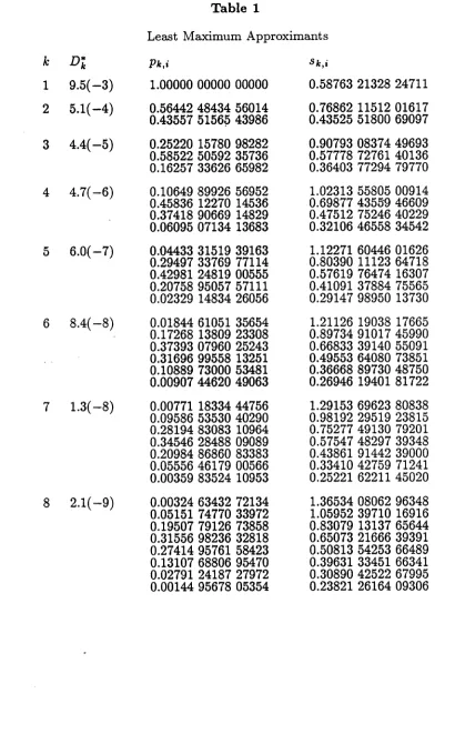
4. THE DISCRETE MIXTURE APPROXIMATION

The lea3t-maxirnum approximant, Fk' minimizes D'k

=

SUPt

I

Dk(t)

I,

where Dk(t)

=

F(t) - Fk(t) subject to the parametric constraints on _Fk. Since Dk(t) is skew-symmetric,

D'k is determined by the restriction of Dk to [0, 00).

Least-maximum approximations form the basis for computing all nonarithmetic

func-tions wherein the approximant is usually a polynomial or rational function. In the case

of a polynomial of degree m, the solution to the' optimization problem is characterized

by Chebyshev's Alternation Theorem

(Hart,

Cheney, Lawson, Maehley, Mesztenyi, Rice,

Thatcher, and Witzgall, 1968, p. 45), which states that the difference function must have m

+

1 roots and m

+

2 local extrema, equal in magnitude and alternating in sign.

For our problem the approximantFk is not polynomial nor is it linear in the m = 2k-1

parameters {(Pk,i' Sk,i)f=l: 0:5Sk,i; 0:5 Pk,i :5 1,

E~=l

Pk,i

=

I}. Chebyshev's Theorem

does not apply but we conjecture that the least-maximum approximant has local extrema

equal in magnitude and alternating in sign as in the polynomial case. Thus we solved

for approximants _Fk having difference functions Dk possessing m roots in addition to the

(8)

We adapted Remes' Second Algorithm (Hart, et al., 1968, p.45) for finding polynomial

least-maximum approximants in our problem. Given initial values

{P1~L s1~~}f=1

such that the initial difference function DiO) has m + 1 sign-alternating extrema not necessarily

of equal magnitude, m roots of DiO), z~O),

(i

= 1, ... , m) were found. Then, letting

z~O)

=

°

and

Z~~l

= z* for some large z*, the m + 1 extrema

x~O)

of DiO) in the intervals

(Zi-l, Zi),

(i

=

1, ... , m+1) were found. Updated parameters

{Pk~L sk~~H=1

were obtained

by solving the m + 1 nonlinear equations

(i=1, ... ,m+1), (4.1)

as functions of the m + 1 arguments {pk,i, 8k,il~=1 and D. This three-step procedure was iterated until convergence. At the stationary point, Dk had the requisite number of

sign-alternating, equal-magnitude extrema, giving us reason to believe that the least-maximum approximant on (0, z*) was found. Since for z* sufficiently large, Dk is negative and

monotonically increasing to zero, the restriction to (0, z*) is not binding and our error

estimates apply to (0, 00).

The parameters of the approximations, and the maximum absolute differences

D'k

for k

=

1, ... ,8 are given in Table 1. Note that 81,1

=

0.58763 is slightly smaller than the logistic/normal scale correction given by Cox (1970, p.28) and agrees closely with the factor 16V3/157r= 0.58808 given by Johnson and Kotz (1970, p. 6).

Figure 1 displays a graph of the functions

J (t) - Dk(t)

+

2k - 1

k D* ,

k

(k

=

1, ... ,8),

(4.2)

illustrating the oscillations in

D

k (·),

(k

= 1, ... ,8).

(9)

using a nonlinear least squares routine to minimize a discrete approximation to the L

_zr

norm ofDk • Acceptable starting values were obtained with r

=

1; however, better starting

values were found for r = 2, ... ,4, a consequence of the approximate equivalence of the

sup norm and L2r norm for r large.

In the usual applications of the algorithm, the approximant is either polynomial or a

rational function in which cases the equations in (4.1) are linear or can be replaced with

a linear system in all of the parameters except D (Cody, Fraser, and Hart, 1968). In our

appli~ationthe equations are nonlinear in all the parameters, thereby complicating this step of the algorithm.

5. LOGISTIC REGRESSION MEASUREMENT ERROR MODELS

5.1 Comparison with other approximations

.Other approximations have been proposed for the integral in (2.1). Fuller (1987, p.

262) proposed the Taylor series approximation,

(5.1)

and Carroll and Stefanski (1989) proposed a range-preserving modification to the above

approximation,

(5.2)

The approximations in (5.1) and (5.2) are compared to those in (2.2) in Figure 2. Here we

have graphed the functions

for the various approximations over the range 0.01

<

T

<

5. The eight nearly-linear graphs

(10)

in (5.1) and (5.2) are drawn with dashed lines; the remaining curve (dot-dash) corresponds to the approximation derived from using 20-point Gauss-Hermite quadrature to evaluate (2.1). The "exact" evaluation of (2.1) was obtained using the method proposed by Crouch and Spiegelman (1990) with accuracy set at 10-15 _{and also by an adaptive Simpson's rule}

with convergence criterion set at 10-15_• _{The latter two differed by less than} _10-14 _across

the range ofT values. The two Taylor series approximations are exact at T = 0 and thus more accurate for very small T; however, they quickly breakdown as T increases from zero.

5.2 Example

We have fit, via maximum likelihood, the logistic regression measurement error model (2.1) to several data sets using the approximations in (5.1), (5.2) and those in (2.2), and compared these fits to those obtained from an "exact" fit of (2.1) using the Simpson's rule evaluation mentioned above. In .these data sets,_ f was not large and the differences between -all the estimated models was generally small. However, although the differences between the approximate fits (2.2) for k

=

4, ... ,8 and the exact fit were numerically negligible, differences between the Taylor series approximations (5.1) and (5.2) and the exact fit were occasionally more noticeable, even though the differences were generally

(11)

estimate.

Finally we note that maximum likelihood estimation and large-sample inference in model (2.1) involves evaluation of not only the integral in (2.1) but also the first- and pos-sibly second-order partial derivatives of(2.1)with respect to TJ and'T. The approximations

in (2.2) have the advantage that all the required derivatives have closed-form expressions, thus making them computationally more attractive than other forms of numerical integra-tion.

REFERENCES

Armstrong, B. (1985). Measurement error in the generalized linear model.

Communica-tions in Statistics,

B, 14,

529-544.

Carroll, R. J., Spiegelman, C., Bailey, K., Lan, K. K. G. and Abbott, R. D. (1984). On errors-in-variables for binary regression models. Biometrika, 71, 19-26.

Carroll, R. J. and Stefanski, L. A. (1989). Approximate quasilikelihood estimation in measurement error models. Journal of the American Statistical Association, To

appear.

Cody, W. J., Fraser, W. and Hart, J. F.(1968). Rational Chebyshev approximations using linear equations. Numerische Mathematik, 12, 242-251.

Cox, D. R. (1970). Binary Regression. Chapman and Hall, London.

Crouch, A. and Spiegelman, D. (1990). The evaluation of integrals ofthe form

J

f(t)e-

t2

dt.

Application to logistic-normal models. Journal of the American Statistical Asso-ciation, To appear.

Fuller, W. A. (1987). Measurement Error Models. Wiley, New York.

Gradshteyn, I. S. and Ryzhik, I. W. (1965). Tables of Integrals, Serie3 and Products.

Academic Press: New York

Hart, J. F., Cheney, E. W., Lawson, C. L., Maehley, H. J., Mesztenyi, C. K., Rice, J. R., Thatcher, H. G. and Witzgall, C. (1968). Computer Approximations. Wiley: New York.

Johnson, N. L. and Kotz, S. (1970). Distributions in Statistic3, Continuous Univariate Distributions, Vol. 2. Boston: Houghton-Mifflin.

McCullagh, P. (1989). Binary data, dispersion effects and the sexual behaviour of Ap-palachian salamanders. Technical Report No. 227, Department of Statistics, Uni-versity of Chicago.

Ochi, Y. and Prentice, R. L. (1984). Likelihood inference in a correlated probit regression model. Biometrika, 71, 531-543.

(12)

Report No. 46, Department of Statistics, Oregon State University.

Prentice, R. L. (1986). Binary regression using an extended beta-binomial distribution, with discussion of correlation induced by covariate measurement errors. Journal

of the American Statistical Association, 394, 321-327.

Prentice, R. L. (1988). Correlated binary regression with covariates specific to each binary observation. Biometrics, 44, 1033-1048.

Schafer, D. (1987). Covariate measurement error in generalized linear models. Biometrika,

74, 385-391.

Spiegelman, D. (1988). Design and analysis strategies for epidemiologic research when the exposure variable is measured with error. Unpublished Ph.D. thesis, Department of Biostatistics, Harvard University.

Stefanski, L. A. and Carroll, R.

J.

(1985). Covariate measurement error in logistic regres-sion. Annals of Statistics, 13, 1335-1351.

Stiratelli, R., Laird, N. M. and Ware,

J.

H. (1984). Random-effects models for serial observations with binary response. Biometrics, 40, 961-971.

Williams, D. A. (1982). Extra-binomial variation in logistic lineat models. Applied

Statis-tics, 31, 144-148.

(13)

Table 1

Least Maximum Approximants

k D*_k Pk,i Sk,i

1 9.5(-3) 1.00000 00000 00000 0.58763 21328 24711

2 5.1(-4) 0.56442 48434 56014 0.76862 11512 01617 0.43557 51569 43986 0.43525 51800 69097

3 4.4(-5) 0.25220 15780 98282 0.907930837449693 0.5852250592 35736 0.57778 72761 40136 0.16257 33626 65982 0.36403 77294 79770

4 4.7(-6) 0.10649 89926 56952 1.02313 55805 00914 0.45836 12270 14536 0.698774355946609 0.37418 90669 14829 0.47512 75246 40229 0.06095 07134 13683 0.3210646558 34542

5 6.0(-7) 0.04433 31519 39163 1.12271 60446 01626 0.29497 33769 77114 0.80390 11123 64718 0.42981 24819 00555 0.57619 76474 16307 0.20758 95057 57111 0.41091 37884 75565 0.02329 14834 26056 0.29147 98950 13730

6 8.4(-8) 0.01844 61051 35654 1.21126 19038 17665 0.17268 13809 23308 0.897349101745990 0.3739307960 25243 0.66833 39140 55091 0.31696 99558 13251 0.49553 64080 73851 0.10889 73000 53481 0.36668 89730 48750 0.00907 44620 49063 0.26946 19401 81722

7 1.3(-8) 0.007711833444756 1.29153 69623 80838 0.09586 53530 40290 0.98192 29519 23815 0.2819483083 10964 0.75277 49130 79201 0.3454628488 09089 0.5754748297 39348 0.2098486860 83383 0.43861 91442 39000 0.05556 46179 00566 0.33410 42759 71241 0.00359 83524 10953 0.25221 62211 45020

(14)

Table 2

Comparison of Approximations

Case 1 Case 2

G

fil s.e·CfiI) t-ratio fil s.e·Cfit> t-ratio

GTS 1.4639 0.5663 2.5850 2.8670 0.8286 3.4601

GRPTS 1.4641 0.5667 2.5837 2.8743 0.8442 3.4046

G I 1.4474 0.5504 2;6299 2.8109 0.8012 3.5085

G2 1.4572 0.5663 2.5733 2.8450 0.8334 3.4138

Ga 1.4637 0.5667 2.5829 2.8509 0.8308 3.4313

G4 1.4639 0.5665 . 2.5841 2.8509 0.8308 3.4316

Gs 1.4639 0.5665 2.5841 2.8509 0.8308 3.4316

G6 1.4639 0.5665 2.5841 2.8509 0.8308 3.4316

G7 1.4639 0.5665 2.5841 2.8509 0.8308 3.4316

Gs 1.4639 0.5665 2.5841 2.8509 0.8308 3.4316

(15)

(16)

25

20

15

· .

·

.

• • • • • • "0· • • • • • • • • • • • • • • : • • • • • • • • • • • • • •

·

.

·

.

• • • • • • • • • • • • • • •• • • • • • • • • • • • 0_• • • • • • • • • • • • • • • •

·

.

· .

·

.

10

Figure 1

• • •, • • • • • • • • • • • • • • 0° • •0• • • • • • • • • • • •"0• • • • • • • • • • • • • •

· .

.

· .

.

· .

.

... r···°0° • • • • • • • • • • • • • •0° • • • • • • • • • • • • • •