HATCH, ANDREW GRAYDON. Model Development and Control Design for Atomic
Force Microscopy. (Committee Chair: Ralph C. Smith)
The development of energy-based models and model-based control designs
neces-sary to achieve present and projected applications involving atomic force microscopy
is investigated. Applications include real-time product diagnostics or monitoring
of biological processes, nanoelectromechanical systems (NEMS) and employment of
atomic force microscope (AFM) technology for spintronics. A crucial component in
the AFM design is the piezoceramic (PZT)-based stage used to position the sample.
Whereas PZT actuators provide the broadband and extremely high set point
capa-bilities required by the AFM stages, they also exhibit frequency-dependent hysteresis
and constitutive nonlinearities.
To characterize the field-polarization relation in PZT, low-order macroscopic
mod-els are constructed based on a combination of energy analysis at the mesoscopic level
along with stochastic homogenization techniques. To account for nonuniformity and
inhomogeneities in the material, local coercive field values are assumed to be
dis-tributed. Due to interactions among the dipoles, the effective field is also assumed to
be distributed. Previous work has employed specific functions to describe these
distri-butions. However, the fact that these choices are not based on energy considerations,
The equation of motion for the rod can be derived using force balancing with boundary
conditions determined from the fact that the rod is fixed at one end and pushes against
the stage at the other.
At low frequencies, the hysteresis and constitutive nonlinearities inherent in PZT
can be accommodated through PID or robust control designs. However, at the higher
frequencies required by the previously outlined applications, increasing noise-to-data
ratios and diminishing high-pass characteristics of control filters preclude a sole
re-liance on feedback laws to eliminate hysteresis. This motivates the development of
control designs that incorporate and approximately compensate for hysteresis through
model inverses employed as filters to linearize transducer responses for linear robust
control design and PID control design. The inverse models are also tested in an open
DESIGN FOR ATOMIC FORCE MICROSCOPY
by
Andrew G. Hatch
a dissertation submitted to the graduate faculty of
north carolina state university
in partial fulfillment of the
requirements for the degree of
doctor of philosophy
applied mathematics
raleigh, north carolina
September 2004
approved by:
R.C. Smith
chair of advisory committee
K. Ito
The author was born in Lake Forest, Illinois and has lived most of his life in Raleigh,
NC. He attended North Carolina State University, where he received the degrees of
Bachelor of Science in Mathematics and Bachelor of Science in physics in 1996. He
went on to receive the degree of Master of Science in Applied Mathematics from
North Carolina State University in 2000. After spending nearly two years working
as a tutor at Triangle Learning Consultants and a software consultant at Intelligent
Information Systems, he returned to NCSU in 2002 to complete his doctoral work.
I would like to thank my advisor Dr. Ralph C. Smith as well as the members of the
committee Dr. Kazufumi Ito, Dr. Zhilin Li and Dr. Hien T. Tran. I would also
like to thank my late father Dr. George G. Hatch, my mother Susan, my brothers
Timothy and Jonathan, my friend Mike Zager and my wife Elena.
List of Figures vi
1 Introduction 1
2 Model Development 9
2.1 Constitutive Relations . . . 9
2.2 Well-Posedness Analysis . . . 15
2.3 Parameter Estimation Problem . . . 19
2.4 Coupled Electromechanical Constitutive Relations . . . 20
2.5 Actuator Models . . . 21
2.5.1 Stacked Actuator . . . 21
2.5.2 Cylindrical Actuator . . . 24
3 Approximation Techniques and Implementation Algorithms 29 3.1 Approximation Techniques for Polarization Model . . . 30
3.2 Model Inversion . . . 38
3.3 Parameter Estimation Techniques . . . 41
3.3.1 Estimation of Densities by Constrained Optimization . . . 41
3.3.2 Estimation of Joint Density . . . 42
3.3.3 Estimation of Joint Density with Regularization . . . 45
3.4 Approximation Techniques for Rod Model . . . 46
3.4.1 Complete Rod Model . . . 46
3.4.2 Lumped Rod Model . . . 52
3.5 Approximation Techniques for Shell Model . . . 54
4 Model Validation and Device Characterization 56 4.1 Field-Polarization . . . 56
4.1.2 General Densities, Identification Using Major and
Rayleigh Loops . . . 60 4.1.3 Lognormal/Normal Densities, Identification Using
All Seven Loops . . . 60 4.1.4 General Densities, Identification Using All Seven
Loops . . . 63 4.1.5 Joint Density . . . 65 4.2 Field-Displacement . . . 67
5 PI Control 71
5.1 PI Control Design . . . 71 5.2 Numerical Examples . . . 76
6 Robust Control 80
6.1 Robust Control Design . . . 80 6.2 Numerical Examples . . . 89
7 Open Loop Control 93
7.1 Experimental Design . . . 93 7.2 Experimental Results . . . 94
8 Conclusions and Future Directions 102
List of References 104
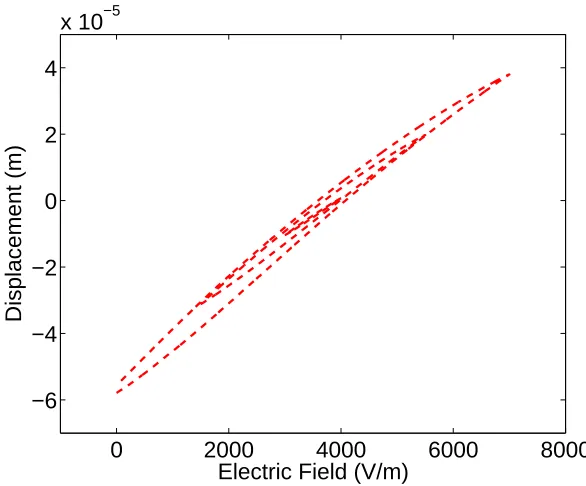
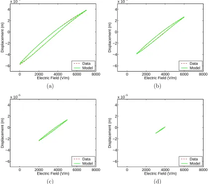
1.1 Schematic of a prototypical atomic force microscope (AFM). . . 2 1.2 Fundamental components in single electron spin microscopy. . . 3 1.3 PZT-based AFM stage. . . 4 1.4 Frequency-dependent field-displacement data from an AFM. Sample
rates of (a) 0.279 Hz, (b) 1.12 Hz, (c) 5.58 Hz, and (d) 27.9 Hz. . . . 5 1.5 Nested minor loops in data collected at 0.1 Hz from an AFM. . . 6
2.1 Gibbs energyGand hysteronP resulting from the necessary condition
∂G
∂P = 0 for negligible thermal activation. . . 11
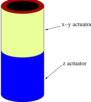
2.2 Cylindrical actuator. . . 25
4.1 PZT5H data collected at 0.2 Hz with a symmetric major loop, Rayleigh loop and five biased minor loops. . . 57 4.2 PZT5H data and model with lognormal and normal densities identified
through a fit to major and Rayleigh loops. . . 59 4.3 Lognormal coercive and normal effective field densities identified through
a fit to major and Rayleigh loops. . . 59 4.4 PZT5H data and model with general densities identified through a fit
to major and Rayleigh loops. . . 61 4.5 General coercive and effective field densities identified through a fit to
major and Rayleigh loops. . . 61 4.6 PZT5H data and model with lognormal and normal densities identified
through a fit to all seven loops. . . 62 4.7 Lognormal coercive and normal effective field densities identified through
a fit to all seven loops. . . 62 4.8 PZT5H data and model with general densities identified through a fit
to all seven loops. . . 64 4.9 General coercive and effective field densities identified through a fit to
all seven loops. . . 64
Ni =Nj = 24 and (b) Ni =Nj = 48. . . 66 4.11 Joint densityνidentified using the quadratic programming formulation
(3.29) for (a) Ni =Nj = 24 and (b)Ni =Nj = 48. . . 66 4.12 PZT5H data and model with joint density ν identified with Tikhonov
regularization using data from all seven loops. (a) Ni =Nj = 24 and (b) Ni =Nj = 48. . . 68 4.13 Joint density ν identified using Tikhonov regularization for (a) Ni =
Nj = 24 and (b) Ni =Nj = 48. . . 68 4.14 Characterization of AFM field-displacement behavior at 0.1 Hz. . . . 69 4.15 Characterization of AFM field-displacement behavior with sample rates
of (a) 0.279 Hz, (b) 1.12 Hz, (c) 5.58 Hz, and (d) 27.9 Hz. . . 70
5.1 On/off control. . . 72 5.2 Proportional control. . . 73 5.3 (a) Disturbance d due to scaled but unmodeled hysteresis and
consti-tutive nonlinearities. (b) Disturbanced due to inverse filtering errors. 75 5.4 P design with no disturbanced and a frequency of 1 Hz. (a) Reference
and simulated trajectory, and (b) tracking error. . . 77 5.5 PI design with no disturbancedand a frequency of 1 Hz. (a) Reference
and simulated trajectory, and (b) tracking error. . . 77 5.6 PI design with disturbanceddue to inversion error and a frequency of
1 Hz. (a) Reference and simulated trajectory, and (b) tracking error. 78 5.7 PI design with disturbance d due to uncompensated hysteresis and
constitutive nonlinearities and a frequency of 1 Hz. (a) Reference and simulated trajectory, and (b) tracking error. . . 78 5.8 PI design with disturbanceddue to inversion error and a frequency of
10 Hz. (a) Reference and simulated trajectory, and (b) tracking error. 79 5.9 PI design with disturbance d due to uncompensated hysteresis and
constitutive nonlinearities and a frequency of 10 Hz. (a) Reference and simulated trajectory, and (b) tracking error. . . 79
6.1 System representation including input disturbancedand sensor noises
and n in the transducer. . . 81 6.2 Linear fractional transformation representation (LFT) of the
trans-ducer model. . . 82 6.3 (a) Frequency response of the passband filter Ws. . . 83 6.4 Frequency response of the highpass filterWn. . . 84
6.6 H2 design with sensor noise s and the disturbance d due to inversion error. (a) Reference and simulated trajectory, and (b) tracking error. 90 6.7 H2 design with sensor noise s and the disturbance d due to
uncom-pensated hysteresis and constitutive nonlinearities. (a) Reference and simulated trajectory, and (b) tracking error. . . 90 6.8 H2 design with sensor noise sbut no disturbance d. (a) Reference and
simulated trajectory, and (b) tracking error. . . 91 6.9 H∞ design with sensor noise s and the disturbance d due to inversion
error. (a) Reference and simulated trajectory, and (b) tracking error. 91 6.10 H∞ design with sensor noise s and the disturbance d due to
uncom-pensated hysteresis and constitutive nonlinearities. (a) Reference and simulated trajectory, and (b) tracking error. . . 92 6.11 H∞design with sensor noisesbut no disturbance d. (a) Reference and
simulated trajectory, and (b) tracking error. . . 92
7.1 (a) Desired displacement with frequency 0.279 Hz and amplitude 40.56µm, displacement achieved with input field determined by inverse model and displacement achieved using input field determined by linear scal-ing. (b) Input field determined by inverse model and input field deter-mined by linear scaling. (c) Tracking error for input field deterdeter-mined from model inverse. (d) Tracking error for input field determined from linear scaling. . . 95 7.2 (a) Desired displacement with frequency 0.279 Hz and amplitude 27.04µm,
displacement achieved with input field determined by inverse model and displacement achieved using input field determined by linear scal-ing. (b) Input field determined by inverse model and input field deter-mined by linear scaling. (c) Tracking error for input field deterdeter-mined from model inverse. (d) Tracking error for input field determined from linear scaling. . . 96 7.3 (a) Desired displacement with frequency 2.79 Hz and amplitude 33.80µm,
displacement achieved with input field determined by inverse model and displacement achieved using input field determined by linear scal-ing. (b) Input field determined by inverse model and input field deter-mined by linear scaling. (c) Tracking error for input field deterdeter-mined from model inverse. (d) Tracking error for input field determined from linear scaling. . . 97
and displacement achieved using input field determined by linear scal-ing. (b) Input field determined by inverse model and input field deter-mined by linear scaling. (c) Tracking error for input field deterdeter-mined from model inverse. (d) Tracking error for input field determined from linear scaling. . . 98 7.5 (a) Desired displacement with frequency 27.9 Hz and amplitude 27.04µm,
displacement achieved with input field determined by inverse model and displacement achieved using input field determined by linear scal-ing. (b) Input field determined by inverse model and input field deter-mined by linear scaling. (c) Tracking error for input field deterdeter-mined from model inverse. (d) Tracking error for input field determined from linear scaling. . . 99 7.6 (a) Desired displacement with frequency 27.9 Hz and amplitude 20.28µm,
displacement achieved with input field determined by inverse model and displacement achieved using input field determined by linear scal-ing. (b) Input field determined by inverse model and input field deter-mined by linear scaling. (c) Tracking error for input field deterdeter-mined from model inverse. (d) Tracking error for input field determined from linear scaling. . . 100 7.7 Data collected before and after open loop experiments at (a) 0.279 Hz
and (b) 27.9 Hz. . . 101
Introduction
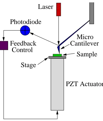
Developed in 1986, the atomic force microscope (AFM), depicted in Figure 1.1, relies
on interatomic forces between a cantilever tip and the sample to obtain ultra-high
res-olution surface images [8]. The relatively low cost of the devices (less than $100,000)
and the fact that they require minimal sample preparation has made the AFM a
standard diagnostic tool in research laboratories. However, several present and
pro-jected applications make requirements on the technology that present AFM designs
are unable to consistently achieve. These limitations are primarily due to the high
sample rates (in the MHz range) required for applications such as real-time product
diagnostics or monitoring of biological processes, nanoelectromechanical (NEMS)
ap-plications, and employment of AFM technologies for spintronics. Real-time product
diagnostics include analysis of contact lenses to detect defects or protein deposits and
screening of semiconductor chips to maintain quality control. The real-time
moni-toring of biological processes has the potential for leading to treatment policies for
ailments such as osteoporosis [31] as well as the potential for quantifying fundamental
biological phenomena such as protein unfolding. Within the NEMS regime, the
repul-sive forces utilized in atomic force microscopy also lead to the potential for
nanocon-struction using the cantilever as an actuator. Finally, the extreme accuracy provided
00 00 00
11 11 11
PZT Actuator Laser
Photodiode
Feedback Control
Micro Cantilever
Sample
Stage
Figure 1.1: Schematic of a prototypical atomic force microscope (AFM).
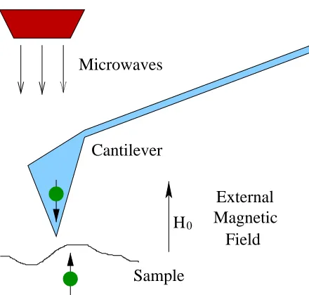
by the AFM is presently being combined with nuclear magnetic resonance microscope
(NMRM) technology to investigate the detection of single electron spins [4, 29, 46]
with the proposed single electron spin microscope (SESM). In the operation of the
SESM, shown schematically in Figure 1.2, an external magnetic field H0 keeps the spins in alignment. Microwave pulses are then used to invert spins in the sample.
The change in force of approximately 10−15 N caused by the inversion of a single spin is detected by the cantilever.
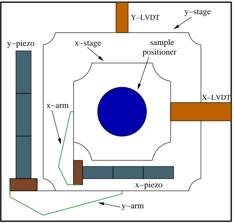
A crucial component in the AFM design for all of these applications is the
piezo-ceramic (PZT)-based stage used to position the sample as depicted in Figure 1.3
[3, 8, 34, 39, 40]. Whereas PZT actuators provide the broadband and extremely
high set point capabilities required by the AFM stages, they also exhibit
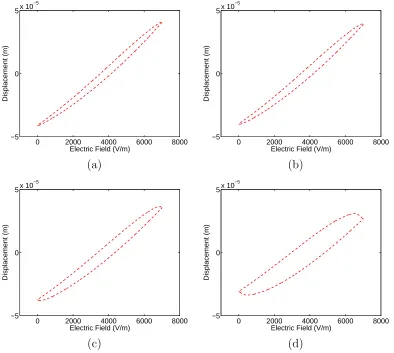
frequency-dependent hysteresis as shown in Figure 1.4. Inertial effects in the rod are clearly
visible in the higher frequency data as evidenced by the observation that the
displace-ments continue to increase for a short time after field reversal. Nested minor loops in
Microwaves
Cantilever
External Magnetic
Field
Sample H0
Figure 1.2: Fundamental components in single electron spin microscopy.
The effects of hysteresis in ferroelectric materials can be greatly reduced or even
nearly eliminated by the use of current or charge controlled amplifiers in place of
voltage controlled amplifiers [15, 16, 17, 18, 19]. However, this approach can be
prohibitively expensive since it requires the construction of specialized amplifiers.
Furthermore, if, as in many applications, there is a need to maintain DC offsets,
cur-rent control will be ineffective. For example, this situation occurs when the x-actuator
in an AFM must be kept fixed while the sample is scanned in the y-direction.
The two goals of this investigation are the development of models that characterize
the hysteresis and constitutive nonlinearities inherent to PZT stages and model-based
control design. We summarize first the state of the art and contributions in each case.
When PZT is placed in the poled state necessary to achieve bidirectional strains,
low to moderate input fields will generate an approximately linear response. The
initial development of linear models characterizing the behavior of piezoelectric
X−LVDT Y−LVDT
y−piezo
x−arm
y−arm x−stage
y−stage sample
positioner
x−piezo
Figure 1.3: PZT-based AFM stage.
A second, more general, framework for characterizing hysteresis and constitutive
nonlinearities is that of domain wall models. Domain wall models involve two basic
mechanisms, domain wall bending, which is reversible, and domain wall translation,
which is irreversible. The theory developed in [36, 37, 38] is based on these concepts.
Additional information on the theory of domain processes can be found in [14] while
a historical summary is provided in [36]. The theory is based on work originally
proposed by Jiles and Atherton for ferromagnetic materials [12].
Preisach methods constitute another general class of models. For example, one of
the first papers studying the application of Preisach models to ferroelectric compounds
was written by Sreeran, Salvady and Naganathan [42] in 1993. An investigation of
Preisach models for PZT, magnetic materials and shape memory alloys (SMAs) was
conducted by Hughes and Wen [11] in 1997. Two examples of extensions of the
0 2000 4000 6000 8000 −5
0
5x 10
−5
Electric Field (V/m)
Displacement (m)
0 2000 4000 6000 8000
−5 0
5x 10
−5
Electric Field (V/m)
Displacement (m)
(a) (b)
0 2000 4000 6000 8000
−5 0
5x 10
−5
Electric Field (V/m)
Displacement (m)
0 2000 4000 6000 8000
−5 0
5x 10
−5
Electric Field (V/m)
Displacement (m)
(c) (d)
Figure 1.4: Frequency-dependent field-displacement data from an AFM. Sample rates of (a) 0.279 Hz, (b) 1.12 Hz, (c) 5.58 Hz, and (d) 27.9 Hz.
Classical Preisach methods are mathematical in structure and are thus very general as
illustrated by Mayergoyz [20, 21], who established mathematical criteria to verify the
applicability of these methods to a variety of magnetic hysteretic situations. Thus,
Preisach models are suitable for characterizing hysteresis in a wide range of materials.
However, the generality of Preisach techniques also creates drawbacks. Since the
parameters in classical Preisach models are not physically based, it is difficult to
0 2000 4000 6000 8000 −6
−4 −2 0 2 4
x 10−5
Electric Field (V/m)
Displacement (m)
Figure 1.5: Nested minor loops in data collected at 0.1 Hz from an AFM.
Another limitation of the classical Preisach formulation is the closure of minor loops,
a phenomenon not always observed in actual materials, where relaxation mechanisms
can prevent this from occurring. For magnetic hysteresis models, extended Preisach
formulations have been developed to address these limitations, although less has been
done for ferroelectric materials in this regard. It should be noted that Preisach models
were developed by Preisach in 1935 for use with magnetic materials [26] and most
early research focused on ferromagnetic materials.
Statistically homogenized energy models provide yet another method for
address-ing hysteresis and these are the type of models that are developed in the present
investigation. It is demonstrated in [39] that these models provide an energy basis for
Preisach models. However, the limitations of the Preisach model can be addressed
Chapter 2 contains the constitutive model development, based on theory
previ-ously developed in [41], and is constructed in three steps. In the first, a Helmholtz
energy relation is derived using statistical mechanics principles under the
assump-tion that dipoles are either aligned with the field or diametrically opposed to it. A
quadratic approximation to this energy is then constructed to facilitate high speed
implementation. In the case of low thermal activation, this leads to a piecewise linear
relationship between the electric field E and the local polarization P. If thermal
activation is significant, the dipoles can change orientation at any time, with the
probability of such a change determined from Boltzmann principles. The number of
dipoles in each orientation evolves according to an ordinary differential equation.
To account for nonuniformity and inhomogeneities in the material, local coercive
field values are assumed to distributed. Due to interactions among the dipoles, the
effective field is also assumed to be distributed. Previous work has employed
spe-cific functions to describe these distributions. For example, lognormal coercive field
densities are common in the magnetics literature and one possible choice for the
ef-fective field density is a normal distribution. However, the fact that neither of these
choices is based on energy considerations motivates the use of general densities. In
this case, the function values of the densities are themselves parameters with the
number of parameters varying according to the desired accuracy. These parameters
must be identified along with the parameter η, which characterizes the slope of the
relationship betweenE and P.
In addition to the hysteresis, the dynamics of the actuator must be incorporated.
For a stacked actuator, such as the one depicted in Figure 1.3, a rod model is suitable
since the cross-section is small compared to the length. The equation of motion for
the rod can be derived using force balancing with boundary conditions determined
from the fact that the rod is fixed at one end and pushes against the stage at the
As discussed in Chapter 3 an approximate solution to the rod equation is found
by first deriving a weak form and then discretizing in space with the finite element
method and in time with finite difference techniques. Approximation techniques and
algorithms for the field-polarization model are also discussed in this chapter.
Chapter 4 addresses model validation for both field-polarization model and the
complete stacked actuator model. For the field-polarization model, a PZT5H data
set collected at 0.2 Hz is used, whereas the AFM data shown in Figures 1.4 and 1.5 is
used for the field-displacement model. The frequency-dependent model is employed
for the data in Figure 1.4.
In addition to characterization, a second goal of the models in the context of the
AFM is to develop model-based control algorithms. At low frequencies, the
hystere-sis inherent to smart materials can be accommodated through
proportional-integral-derivative (PID) or robust control designs [2, 30]. However, at the higher frequencies
required by the previously summarized AFM applications, increasing noise-to-data
ra-tios and diminishing high-pass characteristics of control filters preclude a sole reliance
on feedback laws to eliminate hysteresis. This motivates the development of control
designs that incorporate and approximately compensate for hysteresis through model
inverses employed either in feedback or feedforward loops. Chapters 5 and 6 discuss
PID and robust control design, respectively. In Chapter 7 an open loop control
ex-periment is described. An inverse model is used to predict the appropriate input field
given a desired output field. The prediction is then tested on a stacked actuator. For
comparison, a predicted input field derived by a linear scaling of the desired output
Model Development
In this chapter we develop models for the nonlinear and hysteretic relations between
the electric field and polarization in PZT actuators. An abstract formulation that
defines this model in terms of a compact operator is then described. This leads to an
analysis of the well-posedness of the parameter estimation problem. After a discussion
detailing the coupled elctromechanical constitutive relations, rod and shell actuator
models, which quantify the relation between field and strain, are developed.
2.1
Constitutive Relations
To model the constitutive behavior of the piezoceramic stacked actuator, the
stress-strain relation is assumed to be linear. However, the relation between the applied
field E, or the applied voltage V, and the polarization P exhibits nonlinearities and
hysteresis. The actuator is also biased through poling so that the relation between
P and the strain ε is approximately linear for the considered operating conditions.
To characterize the hysteretic E-P behavior at the domain level, a Helmholtz energy
relation was derived in [41] using statistical mechanics principles under the assumption
that dipoles are either aligned with the field or diametrically opposed to it. This
model is appropriate for a single crystal with uniform effective fields. To construct
a macroscopic model for a polycrystalline material with variable effective fields, the
coercive and effective field values are then assumed to be distributed.
Under fixed temperature conditions with no applied stress σ, it is illustrated in
[41] that a first order approximation to the statistical mechanics-based Helmholtz
energy is the piecewise quadratic relation
ψ(P) =
1
2η(P +PR)2 P ≤ −PI
1
2η(P −PR)2 P ≥PI
1
2η(PI−PR) ³
P2 PI −PR
´
|P|< PI.
(2.1)
As shown in Figure 2.1, PI is the positive inflection point andPR is the polarization
value at which the positive local minimum of ψ occurs. The parameter η is the
reciprocal of the slope of the E-P relation after switching occurs. This fact can be
used to establish an initial parameter value for η when modeling a specific data set.
If there are no applied stresses σ, the Gibbs energy can be formulated as
G(E, P) =ψ(P)−EP, (2.2)
where the second term represents the electrostatic energy due the applied fieldE. In
the case of negligible thermal activation, the local average polarization ¯P is
deter-mined from the necessary conditions
∂G
∂P = 0 , ∂2G
∂P2 >0, (2.3)
ψ(P) = G(0,P) R P I P P 00 00 11 11 00 00 00 11 11 11 P G(E,P) 0 0 1 1 P G(E,P) I P P E c E R P 00 00 00 11 11 11 R c E P P E 0 0 1 1 c E R P E P 0000
00 11 11 11
Figure 2.1: Gibbs energy Gand hysteron P resulting from the necessary condition
∂G
∂P = 0 for negligible thermal activation.
(2.2) yields a piecewise linear E-P characterization
[ ¯P(E;Ec, ξ)](t) =
[ ¯P(E;Ec, ξ)](0), τ(t) =∅
E
η −PR, τ(t)6=∅ and E(supτ(t)) = −Ec E
η +PR, τ(t)=6 ∅ and E(supτ(t)) = Ec
(2.4)
with the initial dipole orientation given by
[ ¯P(E;Ec, ξ)](0) =
E
η −PR, E(0) ≤ −Ec ξ, −Ec < E(0) < Ec
E
η +PR, E(0) ≥Ec
. (2.5)
configurations. The transition times τ are
τ(t) = {t∈(0, tf]|E(t) =−Ec or E(t) = Ec}. (2.6)
The local average polarization can also be written using more compact notation as
P = 1
ηE+δPR, (2.7)
where δ= 1 for positively oriented dipoles and δ =−1 for negative orientations.
However, if thermal activation is significant, the dipoles can achieve the thermal
energy required to switch in advance of the minimum Gibbs energy so the relative
thermal and Gibbs energy must be balanced through Boltzmann principles. The
probability density for achieving an energy level Gis then given by
µ(G) = Ce−GV /kT, (2.8)
wherek is Boltzmann’s constant,V is a reference volume andC is a constant that is
selected so that whenµ(G) is integrated over all possible dipole orientations, a
prob-ability of 1 is achieved. If we let 2σ be the separation between possible polarization
states around P0, the probabilities of reaching a polarization state having sufficient energy to switch orientations from positive to negative, and conversely, are
r+− =
RP0+σ P0−σ e
−G(E,P)V /kTdP R∞
P0−σe−G(E,P)V /kTdP
, r−+ =
RP0+σ P0−σ e
−G(E,P)V /kTdP RP0+σ
−∞ e−G(E,P)V /kTdP
. (2.9)
The rates at which dipoles switch from a positive to a negative orientation and
con-versely are then
p+− = 1
τr+− , p−+=
1
where τ is the relaxation time. The fractions of dipoles in each orientation evolve
according to the ordinary differential equations
dx+
dt =−p+−x++p−+x− , dx−
dt =−p−+x−+p+−x+. (2.11)
The expected polarizations due to positively and negatively oriented dipoles are
hP+i=
Z ∞
P0+σ
P µ(G)dP , hP+i=
Z P0−σ
−∞
P µ(G)dP (2.12)
so the evaluation of C yields
hP+i=
R∞
P0+σP e−G(E,P,T)V /kTdP R∞
P0+σe−G(E,P,T)V /kTdP
, hP−i=
RP0−σ
−∞ P e−G(E,P,T)V /kTdP RP0−σ
−∞ e−G(E,P,T)V /kTdP
. (2.13)
For a single crystal with uniform effective field, the local average polarization is
subsequently
¯
P =x+hP+i+x−hP−i. (2.14)
In the manner detailed in [41], the evaluation of the integrals in (2.9) and (2.13)
can be simplified through approximations employing the inflection points±PI rather
than the unstable equilibrium P0.
Both of the relations (2.4) and (2.14) are valid only for homogeneous single
crys-tal materials with uniform effective fields. To account for nonuniformity and
inho-mogeneities in the materials, local coercive and effective fields are assumed to be
manifestations of underlying distributions rather than constants. The macroscopic
polarization model is then given by
P(E) =
Z ∞
0
Z ∞
−∞
¯
where ν1 and ν2 are appropriate densities.
Motivated by choices in the magnetics literature, ν1 and ν2 were respectively designated to be lognormal and normal densities in [41]; thus
ν1(Ec) = C1e−ln[(Ec/Ec)/2c]2 (2.16)
ν2(Ee) =C2e−(E−Ee)2/b. (2.17)
However, the fact that neither of these choices is based on energy considerations,
motivates the consideration of general densities. Furthermore, as long as the densities
are required to have positive arguments for the coercive field and exhibit certain
decay properties, there is no physical reason why normal and lognormal functions
are inherently preferable to general densities, which provide much greater flexibility
for model construction. Based on physical principles, we assume that the general
densitiesν1 and ν2 satisfy the following conditions
(i) ν1(Ec) is defined for Ec >0 (2.18) (ii) ν2(Ee) = ν2(−Ee) (2.19) (iii) |ν1(Ec)| ≤c1e−a1Ec,|ν
2(Ee)| ≤c2e−a2Ee, (2.20)
where a1, a2, c1 and c2 are nonnegative. The first condition is required since the coercive field Ec must be positive. The second condition reflects the assumption
that the effective field Ee is symmetric. The third condition represents the physical
observation that the coercive and effective fields decay as a function of distance.
This also ensures finite polarization values when integrating the densities against the
2.2
Well-Posedness Analysis
For the general densities defined by conditions (2.18), (2.19), and (2.20), we can also
consider a single joint density function, where the general densitiesν1(Ec) andν2(Ee) are replaced with the joint density ν(Ec, Ee) = ν1(Ec)ν2(Ee) so that (2.15) has the form
P(E) =
Z ∞
0
Z ∞
−∞
¯
P(E+Ee, Ec, ξ)ν(Ec, Ee)dEedEc. (2.21)
Making use of condition (2.20) allows (2.21) to be approximated to arbitrary accuracy
by
P(E) =
ZZ
Ω2 ¯
P(E+Ee, Ec, ξ)ν(Ec, Ee)dEedEc, (2.22)
where Ω2 is the compact domain {(Ec, Ee) ∈ R+×R|ν(Ec, Ee) ≥ ²}. Now let Emin
and Emax be the minimum and maximum allowable input fields and define Ω1 to be the domain [Emin, Emax]. Next define the parameters q=ν in the parameter space
Q=L2(Ω2) (2.23)
and let k=P. Then, let
E ∈C[Ω1]⊂L2(Ω1) (2.24)
and define the observation operator CP =P(E) on the observation space
Y =L2(Pmin, Pmax). (2.25)
Finally, define the parameter-to-observation operatorK by
Kq=C
ZZ
Ω2
The polarization model (2.22) can subsequently be rewritten as
y(E) = Kq(E). (2.27)
Now, define Ω = Ω1 × Ω2 and note that since k has an affine construction,
k ∈L1(Ω)∩L2(Ω). The first property is typical for convolution operators. The sec-ond property allows easier construction of a generalized Fourier basis, which will be
used in showing that the operator K is compact. Note that K is a special case of a
Hilbert-Schmidt operator and has kernel in L2. The proof that follows is a modifica-tion of the proof in [10] for Hilbert-Schmidt operators with kernels in L2(R2n). We
first summarize Theorem 5.24.8 from [22]:
Theorem 1 Let X and Y be Banach spaces and let KN : X → Y, N = 1,2,· · ·, be a sequence of compact linear operators converging to a bounded linear operator
K : X → Y; that is, kKN − Kk → 0 as N → ∞. Then K is a compact linear
operator.
Thus, to show thatKis a compact operator, it must be demonstrated thatKis the
limit of a sequence of finite operators. The first step is to construct an orthonormal
basis{φi}forL2(Ω). It is demonstrated in [22] that an orthonormal basis forL2(Ω1) is
ϕ`(s) = √ 1
Emax−Eminexp ·
2πi`· s−Emin Emax−Emin
¸
, `= 0,±1,±2,· · · . (2.28)
An orthonormal basis for L2(Ω2) can be created in an analogous manner. Thus, an orthonormal basis forL2(Ω) is
φ`m(s, t, v) = ϕ`(s)ϕm(t, v). (2.29)
written in the generalized Fourier series form
f =X
i
hf, φiiφi. (2.30)
From Plancheral’s theorem, it follows that
kfk2 =X
i
|hf, φii|2. (2.31)
Letting ψi = Kφi, allows K and the approximating finite-rank operators KN to be
represented by
Kf =X
i
hf, φiiψi (2.32)
KNf = N X
i=1
hf, φiiψi. (2.33)
Then,
X
i
kψik2 =X
i ·Z
Ω1|K
φi(E)|2dE ¸
=X
i Z
Ω1
¯¯
¯¯ZZΩ2k(E+Ee, Ec)φi(Ec, Ee)dEedEc¯¯¯¯
2
dE
=
Z
Ω1
" X
i ¯¯
¯¯ZZΩ2k(E+Ee, Ec)φi(Ec, Ee)dEedEc¯¯¯¯
2#
dE
=
Z
Ω1
·ZZ
Ω2|
k(E+Ee, Ec)|2dEedEc ¸
dE <∞,
where the last step follows using Plancheral’s theorem. There thus existsLsuch that
X
i
kψik2 →L (2.35)
and thus
X
i≥N+1
kψik2 →0, as N → ∞. (2.36)
Therefore, for ε >0, there exists Nε such that for N > Nε,
kK − KNk= sup f6=0
kKf − KNfk
kfk < ε. (2.37)
From this it can be concluded that
lim
N→∞kK − KNk= 0 (2.38)
and since the range of KN is finite,KN is a compact operator.
Now we show the convergenceK → KN. Using the Schwartz inequality, note that
kKf− KNfk=
°° °° °
X
i≥N+1
hf, φiiψi °° °° °
≤ X
i≥N+1
|hf, φii| kψik
≤
" X
i≥N+1
|hf, φii|2 #1
2 " X
i≥N+1 kψik2
#1 2
≤ kfk "
X
i≥N+1 kψik2
#1 2
.
(2.39)
Thus by Theorem 1,K is a compact operator since it is the norm limit of a sequence
2.3
Parameter Estimation Problem
Given data (E,b Pb), where Eb ∈ L2(Emin, Emax), the parameter estimation problem is to find q∈ Qsuch that
Kq=P .b (2.40)
There is a classical solution to this problem if and only if Pb ∈ R(K), whereR(K) is
the range of K. Since this will not be true in general, the least squares formulation
min
q∈QT(q), T(q) =
1
2kKq−Pbk
2 (2.41)
is typically more appropriate. However, even this problem is ill-posed since the fact
that K is compact with infinite-dimensional range makes the Moore-Penrose inverse
K† discontinuous [7]. One way to deal with this difficulty is to solve the regularized
problem
min
q∈QTα(q), Tα(q) =
1
2kKq−Pbk
2+αJ(q), (2.42)
where the additional termαJ(q) provides stability. As the regularization parameter
α >0 is increased, stability increases as well, but at the cost of reducing the quality
of the characterization of the data. One choice for J is the Tikhonov functional
J(q) = 1 2kqk
2. (2.43)
Implementation of (2.42) with Tihonov regularization for data collected on PZT5H
2.4
Coupled Electromechanical Constitutive
Relations
To include ferroelastic coupling, we utilize the extended Helmholtz relation
ψe(P, ε) =ψ(P) + 1 2Y
Pε2 −YPγεP, (2.44)
where ψ(P) is given by (2.1). The Gibbs energy is then
G(E, P, ε) = ψ(P) + 1 2Y
Pε2−YPγεP −EP −σε, (2.45)
where the term σε incorporates the elastic energy. Note that YP is the Young’s
modulus for a constant polarization andγ is a ferroelastic coupling coefficient.
The equilibrium condition
∂G
∂ε = 0 (2.46)
yields the elastic constitutive relation
σ=YPε−YPγP. (2.47)
This relation along with the nonlinear polarization relation (2.15) quantifies the
con-stitutive behavior for the piezoceramic materials employed in the AFM.
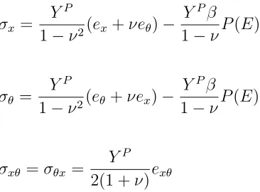
When a PZT shell is employed for actuation instead of a rod, longitudinal strains
The 2-D constitutive relations for the shell are
σx = Y
P
1−ν2(ex+νeθ)− YPβ
1−νP(E)
σθ = Y
P
1−ν2(eθ+νex)− YPβ
1−νP(E) (2.48)
σxθ =σθx = Y
P
2(1 +ν)exθ
with the relation for P(E) given by (2.15). Here, εx, σx, εθ and σθ represent the
normal strains and stresses in the longitudinal and circumferential directions, while
the shear strains and stresses are denoted byexθ and σxθ. Also,ν is the Poisson ratio
for the material andβ is the electromechanical coupling coefficient.
2.5
Actuator Models
In addition to hysteresis, the dynamics of the actuator must be incorporated. Stacked
actuators, which create motion in only one direction, are employed in pairs as in
Figure 1.3 so that the stage can be moved in both the x and y directions. The
cylindrical actuator is poled to generate movement in both directions by itself.
2.5.1
Stacked Actuator
For the stacked actuator, we assume that the rod has cross-sectional areaA, length`,
density ρ and Young’s modulusYP. LetcP be the Kelvin-Voigt damping parameter
and γ be the piezoelectric coupling coefficient. In the present stage design, depicted
in Figure 1.3, one end of the actuator is fixed, while the attachment at the other
c` respectively denote the mass, stiffness and damping coefficients. Force balancing
along the actuator then yields the relation
ρA∂
2u
∂t2 = ∂N
∂x , (2.49)
where the resultant N =RAσdA is given by
N =YPA∂u ∂x +c
PA ∂2u ∂x∂t −Y
PAγP(E). (2.50)
Note that u denotes the displacement in the longitudinal x-direction and that the
relation strain ε = ∂u∂x is used in obtaining (2.50). The boundary conditions are
u(t,0) = 0 (2.51)
at the fixed end and
N(t, `) =−k`u(t, `)−c`∂u
∂t(t, `)−M` ∂2u
∂t2(t, `) (2.52)
at the moving end. Initial conditions are given by
u(0, x) = ∂u
∂t(0, x) = 0. (2.53)
The polarization P(E) is specified by (2.15).
To provide a setting that facilitates approximation, we also derive a weak
for-mulation as described below in a manner similar to that in [39]. Let the states
z = (u(·), u(`)) be in the space X =L2(0, `)×R, where the inner product is defined by
hξ1, ξ2iX =
Z `
0
and let the space of test functions be
V ={Ψ = (ψ, ϕ)∈X|ψ ∈H1(0, `), ψ(0) = 0, ψ(`) =ϕ}, (2.55)
where the inner product is defined by
hΨ1,Ψ2iV =
Z `
0
YPAψ10ψ02dx+k`ψ1(`)ψ2(`). (2.56)
Multiplying (2.49) by ψ ∈H01(0, `) ={ψ ∈H1(0, `)|ψ(0) = 0}and integrating gives
Z `
0
ρA∂
2u
∂t2ψdx= Z `
0
∂N
∂xψdx. (2.57)
Then, integrating the right side by parts,
Z `
0
ρA∂
2u
∂t2ψdx=ψN | ` 0− Z ` 0 N ∂ψ ∂xdx
=ψ(`)N(t, `)−ψ(0)N(t,0)−
Z `
0 N
∂ψ ∂xdx
=ψ(`)N(t, `)−
Z `
0 N
∂ψ ∂xdx,
where the fact thatψ(0) = 0 is used in the last step. Substituting for N from (2.50)
and for N(t, `) from (2.52) yields
Z `
0
ρA∂
2u
∂t2ψdx=ψ(`) ·
−k`u(t, `)−c`∂u
∂t(t, `)−M` ∂2u
∂t2(t, `) ¸
−
Z `
0
·
YPA∂u ∂x +c
PA ∂2u ∂x∂t −Y
PAβP (E) ¸
Rearranging terms gives the weak form
Z `
0
ρA∂
2u
∂t2ψdx+ψ(`)M` ∂2u
∂t2(t, `) + Z `
0
·
YPA∂u ∂x +c
PA ∂2u ∂x∂t
¸ ∂ψ ∂xdx
+ψ(`)
·
k`u(t, `) +c`∂u ∂t(t, `)
¸
=
Z `
0
YPAβP(E)∂ψ
∂xdx, (2.58)
which must hold for all ψ ∈ V. An approximation to the weak form (2.58) is found
by discretizing in space with linear finite elements and in time with finite difference
techniques as described in Section 3.4.
2.5.2
Cylindrical Actuator
Consider a cylindrical actuator composed of two shells stacked one on top of the other
as depicted in Figure 2.2. The first shell creates displacements in the x-y direction
while the second shell actuates in the z direction. Motions in the latter direction
are used to maintain constant force between the sample and the micro-cantilever on
the AFM. When analyzing the dynamics for this case, the mass of the x-y shell is
combined with the mass of the sample to yield a total mass m, which acts as an
inertial force at the free end of the z shell.
Assume that thez shell has length`, thicknessh, radiusR, densityρand Young’s
modulusYP. Let Γ
0 = [0, `]×[0,2π] represent the reference or neutral surface of thez shell. The longitudinal, circumferential and transverse displacements are denoted by
u, v and w. Consider the case where the bottom of the z shell (x= 0) is fixed, while
the top (x=`) is free. Thus the motion of the top depends only on the inertial force
of the combined mass m of the x-y shell and the sample. In the model development
which follows, internal damping is assumed to be absent. However, descriptions of
how to include Kelvin-Voigt damping by assuming that stress is a linear combination
x−y actuator
z actuator
Figure 2.2: Cylindrical actuator.
The derivation of the Donnell-Mushtari shell equations
Rρh∂
2u
∂t2 −R ∂Nx
∂x −
∂Nxθ ∂θ = 0
Rρh∂
2v
∂t2 − ∂Nθ
∂θ −R ∂Nxθ
∂x = 0 (2.59)
Rρh∂
2u
∂t2 −R ∂Mx
∂x2 −
1
R ∂2Mθ
∂θ2 −2
Mxθ
∂x∂θ +Nθ = 0
from force and moment balancing is described in [1]. Here, Nx, Nθ and Nxθ are
general force resultants and Mx, Mθ and Mxθ are moment resultants. Boundary
conditions are enforced atx= 0 and x=`. For x= 0
u=v =w= ∂w
and for x=`
Nx =−m ∂2u
∂t2 Nxθ+
1
RMxθ = 0
Qx+
1
R ∂Mxθ
∂θ = 0 Mx = 0,
where the first condition at x = ` incorporates the inertial force from the combined
mass m. To determine the force and moment resultants when there are no shear
stresses, the stress relations (2.48) are integrated through the thickness of the shell
to give
Nx= YPh
1−ν2(ex+νeθ)− YPhβ
1−νP(E) (2.61)
Nθ = YPh
1−ν2(eθ+νex)− YPhβ
1−νP(E) (2.62)
Nxθ =
YPh
2(1 +ν)exθ (2.63)
and
Mx =
YPh3
12(1−ν2(κx+νκθ) (2.64)
Mθ =
YPh3
12(1−ν2)(κθ+νκx) (2.65)
Mxθ =
YPh3
In addition, the midsurface strains and changes in curvature are
ex = ∂u
∂x κx =−
∂2w ∂x2
eθ = 1
R µ
∂v ∂θ +w
¶
κθ =− 1
R2 ∂2w
∂θ2
exθ = ∂v
∂x +
1
R ∂u
∂θ τ =−
2
R ∂2w ∂x∂θ.
An approximate solution to (2.59) is found by first deriving a weak form as described
in [39] and summarized here. First, let the state space be
X =L2(Γ0)×L2(Γ0)×L2(Γ0). (2.67)
Then let φ = (u, v, w) and ψ = (η1, η2, η3) and define the inner product
hφ, ψiX =
Z
Γ0
ρhuη1dγ +
Z
Γ0
ρhvη2dγ+
Z
Γ0
ρhwη3dγ+muη1(`). (2.68)
Next, define
H`1(Γ0) = {η∈H1(Γ0)|η(0, θ) = 0}
H`2(Γ0) = {η∈H2(Γ0)|η(0, θ) = ηx(0, θ) = 0}
and let the space of test functions be
Define the inner product on this space as
h(YP)φ, ψiV =
Z
Γ0
YPh
1−ν2 ·
(ex+νeθ)∂η1
∂x +
1
2R(1−ν)exθ ∂η1 ∂θ ¸ dγ + Z Γ0
YPh
1−ν2 ·
(eθ+νex)∂η2
∂θ +
1
2R(1−ν)exθ ∂η2 ∂x ¸ dγ + Z Γ0
YPh
1−ν2 ·
1
R(eθ+νex)η3− h2
12(κx+νκθ)
∂2η3 ∂x2
− h2
12R2(κθ+νκx) ∂2η3
∂θ2 − h2
12R(1−ν)τ ∂2η3 ∂x∂θ
¸ dγ.
(2.70)
The weak form of the model (2.59) can then be written as
Z
Γ0
· Rρh∂
2u
∂t2η1 +RNx ∂η1
∂x +Nxθ ∂η1
∂θ −R YPhβ
1−νP(E) ∂η1
∂x ¸
dγ
−Rm∂
2u
∂t2η1(`) = 0 Z
Γ0
· Rρh∂
2v
∂t2η2+Nθ ∂η2
∂θ +RNxθ ∂η2
∂x − YPhβ
1−νP(E) ∂η2
∂θ ¸
dγ = 0
Z
Γ0
· Rρh∂
2w
∂t2 η3+Nθη3−RMx ∂2η3
∂x2 −
1
RMθ ∂2η3
∂θ2 −2Mxθ ∂2η3 ∂x∂θ
(2.71)
for all ψ = (η1, η2, η3) ∈ V. An approximation to the weak form (2.71) is found by discretizing in space with a tensored basis comprised of cubic B splines and Fourier
elements and in time with finite difference techniques as described in [39] and
Approximation Techniques and
Implementation Algorithms
In this chapter, we begin by discussing approximation techniques and implementation
algorithms for the field-polarization models described in Chapter 2. The first
ap-proach uses constrained optimization with a least squares cost function to determine
the general density parameters and η. In the second method, the general densities
are combined into a single joint density and the resulting linear system is solved using
the techniques employed in [43] for identifying density functions in Preisach models.
In the final approach, the constrained minimization problem for the joint density
is modified to include Tikhonov regularization to accommodate the ill-posedness of
the original formulation. All three methods are validated with a PZT5H data set
collected at 0.2 Hz. Then an inverse algorithm quantifying the polarization-field
rela-tion is developed for use in control design. Secrela-tion 3.3 addresses parameter estimarela-tion
techniques for the field-polarization algorithms from Section 3.1. Finally,
approxima-tion techniques and implementaapproxima-tion algorithms for the rod and shell actuator models
are outlined.
3.1
Approximation Techniques for Polarization
Model
To implement the nonlinear polarization model (2.15), the integrals must be
approxi-mated. One approach is to use Gaussian quadrature routines constructed for infinite
or semi-infinite domains. Alternatively, the decay of the densities ν1 and ν2 allows the intervals to be truncated so that Gauss-Legendre rules can be employed. Both
cases are described in detail in [41]. In either case, the discrete model will be of the
form
P(E) =
Ni X i=1 Nj X j=1 ¯
P(E+Eej, Eci, ξi)ν1(Eej)ν2(Eci)viwj, (3.1)
where Eej, Eci are the abscissas and vi, wj are the weights. For the characterization examples in the sections which follow, we use a 4 point composite Gauss-Legendre
quadrature rule for truncated domains. For the integral over Ee let the truncated
domain be [−L, L] and letNqj be the number of subintervals for the composite Gaus-sian quadrature. The subintervals are then [hqj−1, hqj], where hqj = −L+qjh with
qj = 1. . . Nqj and h= 2L/Nqj. If we use a four point rule, Nj = 4Nqj and the points and weights on each subinterval are
εqj1 =hqj−1+h "
1 2−
p
15 + 2√30
2√35
#
, wqj1 = 49h
12(18 +√30)
εqj2 =hqj−1+h "
1 2−
p
15−2√30 2√35
#
, wqj2 = 49h
12(18−√30)
εqj3 =hqj−1+h "
1 2+
p
15−2√30 2√35
#
, wqj3 = 49h
12(18−√30)
εqj4 =hqj−1+h "
1 2+
p
15 + 2√30
2√35
#
, wqj4 = 49h
For the integral overEc let the truncated domain be [0, K] and letNqi be the number of subintervals. Here, the subintervals are [gqi−1, gqi], where gqi = qig with qi = 1. . . Nqi and g = K/Nqi. Again using a four point rule, we have Ni = 4Nqi and analogous nodes and weights. If the joint density formulation (2.21) is used, the
discretized version becomes
P(E) =
Ni
X
i=1 Nj
X
j=1
¯
P(E+Eej, Eci, ξi)ν(Eej, Eci)viwj. (3.2)
The number of parameters required for the construction of (3.1) depends on the
choice of densities. For the lognormal and normal densities there are five parameters;
η,C,Ec,candb, whereC =C1C2. Note that for any values ofη,C andPR, rescaling allows PR to be set to 1. Thus, PR does not need to be identified. For the general
densities the Ni +Nj + 1 parameters [ν1(Ec1),· · · , ν1(Ec
Ni)], [ν2(Ee1),· · · , ν2(EeNi)]
andηneed to be identified. The joint density νrequires the identification of NiNj+ 1
parameters. The larger number of parameters in the general density and joint density
formulations allows the construction of models which are highly accurate for a wide
range of drive regimes. The trade off is the increased time and effort required to
identify the parameters. Numerical simulations have indicated that Ni and Nj must
be on the order of 40 to 80 to achieve convergence of (3.1). Therefore, highly efficient
optimization and parameter estimation techniques are required. However,
implemen-tation of the model in control design is equally efficient for both the lognormal and
normal densities and general densities since each involves the multiplication ofNi×1
and Nj ×1 vectors.
An implementation of the forward model (3.1) based on the description in [41] is
now summarized. Formulate the local polarization (2.4) as
P = E
where ∆ is an Ni ×Nj matrix whose elements are either 1 or −1. The ijth entry
in ∆ indicates whether the jth effective field value Eej has crossed the ith coercive field valueEci and thus whether the associated polarization value is on the upper or lower branch of the hysteron. As the field is changed, the entries in ∆ can be updated
either by usingif-thenstatements or by employing the following matrix multiplication
algorithm. First define the matrices,
∆init=
−1 · · · −1 1 · · · 1 ..
. ... ... ...
−1 · · · −1 1 · · · 1
Ni×Nj
εc =
Ec1 · · · Ec1
..
. ...
Ec
Ni · · · EcNi
Ni×Nj
εk =
Ek+Ee1 · · · Ek+Ee
Nj
..
. ...
Ek+Ee1 · · · Ek+Ee
Nj
Ni×Nj
O =
1 · · · 1 ..
. ...
1 · · · 1
Ni×Nj
(3.4)
and the weight vectors
VT =
h
v1ν1(Ec1),· · · , vNiν1 ³
Ec
Ni
´i
1×Ni
(3.5)
WT =
h
w1ν2(Ee1),· · · , wNjν2 ³
Ee
Nj
´i
1×Nj
, (3.6)
where Ek is the kth value of the input field. The calculation of Pk is summarized in
Algorithm 1, where .* denotes componentwise matrix multiplication and sgn is the