SAMU, VIVEK. Nondestructive Length Estimation of Pile Foundation through Effective Dispersion Analysis of Reflections. (Under the direction of Dr. Murthy Guddati).
This dissertation introduces a newly developed method called the Effective Dispersion Analysis of Reflections (EDAR) to effectively estimate the length of unknown foundations. The key idea of the method is based on accurately capturing the dispersion of waves as they
propagate through a pile and is applicable to both longitudinal and bending waves. Specifically, the measured accelerations at two distinct locations on the pile due to hammer impact is
processed using EDAR methodology resulting in an estimate of the pile length (foundation depth).
Firstly, EDAR is derived through simple one-dimensional bar and Bernoulli-Euler beam models and validated through laboratory testing. The analysis hinges on examining the
oscillations in phase difference that are due to reflections, as a function of a newly defined quantity called effective wavenumber, which is essentially a scaled wavenumber. Laboratory experiments on concrete filled steel tubes (CFST) on loose soil conditions resulted in accurate length estimates with less than 5 percent error.
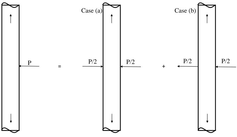
Secondly, based on the success in the lab EDAR was extended to field piles. The original EDAR method is based on processing dispersive bending wave signals in the frequency-effective wavenumber domain, thus eliminating the need to perform peak picking that is difficult due to over-distortion of reflected signals. While the method was successful in laboratory settings, preliminary field validation resulted in significant errors. After careful examination of the wave physics, it is discovered that both longitudinal and transverse waves need to be carefully
included in EDAR analysis. Specifically, it is shown that the initial arrival is dominated by transverse waves, while the reflections are dominated by longitudinal waves, owing to significant attenuation of transverse waves due to compacted soil around the pile. This observation led to a refined EDAR methodology and accurate estimation of embedded pile depth in field settings (less than 10 percent error).
Reflections
by Vivek Samu
A dissertation submitted to the Graduate Faculty of North Carolina State University
in partial fulfillment of the requirements for the degree of
Doctor of Philosophy
Civil Engineering
Raleigh, North Carolina 2019
APPROVED BY:
_______________________________ _______________________________ Dr. Murthy Guddati Dr. Shamim Rahman
Committee Chair
ii DEDICATION
iii BIOGRAPHY
iv ACKNOWLEDGMENTS
I would like to express my deep gratitude to my advisor Dr. Murthy Guddati for his patient guidance, encouragement and useful critiques of this research work. His valuable
suggestions have helped me progress and improve as a researcher over the course of my graduate studies.
I would like to thank Dr. Mervyn Kowalsky, Dr. Shamim Rahman and Dr. Ralph Smith for serving as members of my advisory committee. I would also like to specially thank Dr. Mervyn Kowalsky and Dr. Diego Aguirre Realpe for allowing me to perform tests on piles built for their research at North Carolina State University.
I would also like to thank Mr. Mike Knapp and Mr. Hiram Henry from Alaska Department of Transportation and Mr. Mohammed Mulla and Mr. Chris Krieder from North Carolina Department of Transportation for their continued support in identifying and help in testing of the field piles.
Many thanks to my fellow graduate students Dr. Hao Hu, Dr. Ali Vaziri, Srikrishnan Madhavan, David Zabel, Abhinab Bhattacharjee, Abdelrahman Elmeliegy, and Sriram Guddati who helped me during several laboratory and field tests. I would also like to thank all my friends at North Carolina State University and elsewhere who have supported me throughout my
graduate school.
I would like to thank Keerthana for her unrelenting support and love throughout this journey.
v TABLE OF CONTENTS
LIST OF TABLES ... vii
LIST OF FIGURES ... viii
1 Introduction ... 1
2 Nondestructive Method for Length Estimation of Pile Foundations through Effective Dispersion Analysis of Reflections ... 5
2.1 Introduction ... 5
2.2 Problem Definition and Experimental Set-up ... 7
2.3 Effective Dispersion Analysis of Reflections (EDAR): Theory ... 9
2.3.1 Longitudinal waves in bar ... 9
2.3.2 Flexural waves in beams ... 15
2.3.3 Synthetic examples for EDAR verification ... 18
2.4 Experimental Validation of EDAR ... 20
2.5 Conclusion ... 28
3 Nondestructive Length Evaluation of an Embedded Pile Using Lateral Hammer Impact: Combined Transverse and Longitudinal Waves ... 29
3.1 Introduction ... 29
3.2 EDAR Preliminaries ... 31
3.2.1 Theory ... 32
3.2.2 Laboratory testing ... 35
3.3 Observations from Field Testing ... 38
3.4 The role of longitudinal waves ... 41
3.4.1 Existence of secondary longitudinal modes ... 43
3.4.2 Differential attenuation of waves due to presence of soil ... 47
3.5 Improved length estimation ... 50
3.6 Final Field Validation... 51
3.6.1 Material properties from cycle period ... 51
3.6.2 Length estimate from wiggle period ... 54
3.7 Summary and Conclusions ... 55
4 Experimental aspects of EDAR ... 56
vi
4.1.1 Accelerometers ... 57
4.1.2 Data acquisition system (DAQ) ... 59
4.1.3 Signal processing ... 59
4.2 Hammer characteristics and producing a good impact ... 60
5 Pile test results, Improvements and Extension of EDAR ... 68
5.1 Hollow steel pipes ... 68
5.2 Concrete filled steel tubes (CFST) in laboratory ... 69
5.3 CFST in field conditions – Portage pile and preliminary analysis ... 72
5.4 Effect of top and bottom boundaries ... 76
5.5 Preliminary work for detection of discontinuity ... 81
5.5.1 Preliminary Theoretical Study ... 82
5.5.2 Analysis of Laboratory Data ... 85
6 Summary and Conclusions ... 87
vii LIST OF TABLES
Table 2-1: Model Bernoulli-Euler beam properties ... 18
Table 2-2: Bernoulli-Euler beam model length estimate ... 19
Table 2-3: Properties of concrete filled steel tube ... 21
Table 2-4: Equipment specifications ... 22
Table 2-5: Length estimate from first observed wiggle using Bernoulli-Euler beam theory ... 25
Table 2-6: Average length estimates ... 27
Table 3-1: Length estimates for laboratory pile ... 38
Table 3-2: Field pile properties ... 39
Table 3-3: Properties of soft and hard soil ... 48
Table 3-4: Improved length estimates... 55
Table 4-1: Accelerometer specifications ... 59
Table 4-2: Hammer specifications ... 61
Table 5-1: Properties of Portage pile ... 74
Table 5-2: Portage pile length estimates based on flexural waves assumption ... 74
Table 5-3: Improved length estimated – Portage pile ... 75
Table 5-4: Properties of the composite Timoshenko beam ... 77
viii LIST OF FIGURES
Figure 2-1: Pile and experimental set-up schematic ... 8
Figure 2-2: Schematic of infinite bar ... 10
Figure 2-3: Effective dispersion plot for infinite bar: phase difference vs. effective wavenumber ... 12
Figure 2-4: Semi-infinite bar: single reflection ... 12
Figure 2-5: EDAR plot for semi-infinite bar superimposed on infinite bar ... 13
Figure 2-6: Schematic of Bernoulli-Euler beam model ... 18
Figure 2-7: EDAR plot for synthetic Bernoulli-Euler beam experiment involving bottom reflections ... 19
Figure 2-8: EDAR plot for Bernoulli-Euler beam model: bottom and top reflections ... 20
Figure 2-9: Concrete filled steel tube tested at NCSU ... 21
Figure 2-10: Equipment used for EDAR testing... 22
Figure 2-11: Experimental response: time domain ... 23
Figure 2-12: (a) Representative experimental EDAR plots (b) Finding wiggle and cycle period from EDAR plot ... 24
Figure 2-13: Theoretical dispersion relation: Bernoulli-Euler vs. Timoshenko beam theories ... 25
Figure 2-14: Comparison of Bernoulli-Euler and Timoshenko EDAR plots ... 26
Figure 2-15: Length estimates as a function of frequency ... 27
Figure 3-1: Pile setup (a) Top impact (b) Side impact ... 32
Figure 3-2: EDAR plots for Semi-Infinite bar with characteristic cycle and wiggle periods ... 34
Figure 3-3: Laboratory pile (a) Time history at accelerometers 1 and 4 (b) Time history at accelerometers 2 and 3 (c) Representative EDAR plots ... 37
Figure 3-4: Wiggle period as a function of frequency for large (LH) and small (SH) sledge hammers hard tip ... 37
Figure 3-5: (a) Field piles (b) Equipment and sensor location ... 39
Figure 3-6: Representative EDAR plots from Pile 2 for (a) Sensor spacing of 0.62 m (b) Sensor spacing of 0.15 m ... 40
Figure 3-7: Initial field length estimates – significant underestimation ... 41
ix
Figure 3-9: (a) Side impact (b) Top impact on pile ... 43
Figure 3-10: Lateral impact split into symmetric and antisymmetric loading ... 44
Figure 3-11: (a) Symmetric loading (b)System 1 by applying symmetric boundary conditions (c) System 2 for application of reciprocity ... 45
Figure 3-12: Soil stiffness (a) Soft soil (b) Hard soil ... 48
Figure 3-13: Attenuation coefficient (a) Soft Soil (b) Hard soil ... 49
Figure 3-14: Top effect on EDAR plot and cycle period ... 52
Figure 3-15: (a) Variation in cycle period for Pile 1 (b) Variation in cycle period for Pile 2 (c) Variation in velocity for Pile 1 as a function of sensor spacing for Poisson’s ratio 0.15 (d) Variation in velocity for Pile 2 as a function of sensor spacing for Poisson’s ratio 0.15 (e)Longitudinal wave velocity estimate from cycle period using Timoshenko beam model ... 53
Figure 3-16: Average length estimate (a) Pile 1 (b) Pile 2 ... 54
Figure 4-1: Typical setup and equipment ... 57
Figure 4-2: Accelerometers (a) 333B32 (b) 353C33 ... 58
Figure 4-3: Different hammers used for testing ... 61
Figure 4-4: (a) Time-domain and (b) Frequency-domain representation of the force (c) Frequency content of the force from 500 to 3,000 Hz in logarithmic scale (c) Duration of impact vs maximum force ... 62
Figure 4-5: Outer Banks solid concrete pile (a) Large hammer hard tip (LH) (b) Large hammer soft tip (LS) (c) Small hammer hard tip (SH) (d) Small hammer tough tip (ST) ... 63
Figure 4-6: Average frequency from multiple impacts – Outer Banks pile ... 64
Figure 4-7: Portage CFST pile (a) Large hammer hard tip (LH) (b) Large hammer soft tip (LS) (c) Small hammer hard tip (SH) (d) Small hammer tough tip (ST) ... 65
Figure 4-8: Average frequency from multiple impacts – Portage pile ... 66
Figure 4-9: Comparison of good and bad impacts ... 67
Figure 5-1: (a) Hollow steel pipe piles (b) Acceleration history showing ringing (c) Frequency domain of the acceleration (d) EDAR plot ... 69
x Figure 5-3: (a) Lateral testing [38] and (b) soil compaction on the pile sides reducing pile
soil interaction ... 71
Figure 5-4: (a) Average cycle periods (b) average wiggle periods (b) average length estimates obtained ... 72
Figure 5-5: (a) Bridge in Portage, AK (b) Sensor locations and spacing ... 73
Figure 5-6: Improved length estimates for Portage pile with scatter and average ... 75
Figure 5-7: Theoretical Timoshenko beam with a bottom HS ... 77
Figure 5-8: (a) Theoretical EDAR plot with sudden spike due to top reflection (b) Experimental EDAR plot from Portage pile test showing similar characteristics ... 78
Figure 5-9: Impact below bottom sensor resulting in amplification of tops effects ... 79
Figure 5-10: Comparison of experimental and theoretical EDAR plots obtained from hammer strike below the bottom sensor. ... 80
Figure 5-11: Local tube buckling and fracture in the laboratory pile [38] ... 81
Figure 5-12: BE beam with internal hinge ... 82
Figure 5-13: EDAR plot obtained for reflection only from the hinge ... 83
Figure 5-14: EDAR plot obtained from combined bottom and hinge reflection ... 84
Figure 5-15: Processed phase difference to extract the various periods (a) Slope corrected phase difference (b) Fourier components of the corrected phase difference ... 84
1 Chapter 1
Introduction
The 2017 report card for America’s Infrastructure by American Society of Infrastructure (ASCE) [1], reports that one in eleven of the nation’s bridges are rated as structurally deficient and the average age of the nation’s over 600,000 bridges is 43 years. Also, almost 39% of existing bridges are 50 years or older. Thus, the need for structural health monitoring of bridges in terms of maintenance, repair and rehabilitation is becoming more and more critical. Pile Foundations are the most common type of deep foundations for bridges and are used for various conditions such as loose soil, large loads from structure, lack of space for shallow foundation. The capacity of a pile foundation is directly related to its embedded depth. Reduction in the effective depth of the foundation, especially due to scour, may cause significant reduction in strength and thus compromises the safety of the structure. National Bridge Inventory reports that there are more than 27,000 bridges with unknown foundation as of 2016, which could be
potentially scour susceptible. Several other bridges over land are also expected to have unknown foundation and missing or incomplete records [2]. The scour safety of the bridge cannot be determined until the depth of foundation is known, and in most cases the records do not exist. Also, for bridges over land, repair and rehabilitation require information about the foundation elements. Hence it is beneficial to evaluate the effective embedded length of pile.
Detailed studies by the Florida state department of transportation [3], Olson et all [4] and Rausche [5] , contain a comprehensive list, with basic description, of most of the methods used for estimation of unknown foundation depth. The available methods can be categorized broadly into evidence based and nondestructive evaluation methodologies. Evidence based techniques involve static back calculation method based on pile design procedures and artificial neural network (ANN) specially built based on the available data for a region to arrive at unknown foundation information. Nondestructive evaluation methodologies are further categorized as surface techniques and borehole techniques.
2 assessment, damage identification and length evaluations (see e.g. [6]–[15]). Lack of access to the pile top, and inability to induce purely longitudinal wave modes, increase the complexity in the analysis. Sonic echo and impulse response methods require information about the wave propagation velocity in the pile. While typical values based on the pile material are used, this introduces an inherent error in the estimates. This was addressed by the ultraseismic method which uses several sensors along the side of the pile to identify the initial arrival and reflections with higher confidence. This procedure requires multiple sensors and sufficient spacing between sensors which might not be available for piles with limited exposed lengths. Additionally, inducing a combination of both longitudinal and flexural waves increase the complexity in the patterns observed and subsequent analysis.
3 dispersive flexural waves by Farid [21]. Subhani et al. [22] used a combination of SKM and continuous wavelet transform (CWT), which is another time-frequency analysis technique, to estimate the embedded lengths of electricity poles and observed significant error margins in both the cases, up to 43% in some cases. Sheng-Huoo et al. [23] compares results from sonic echo test using CWT, in the context of longitudinal waves. All the above methods are purely based on signal processing and do not explicitly incorporate the dispersion properties of the waves. Essentially, all surface-based methods still rely on being able to get an identifiable reflection from the pile tip. This is specifically a problem whenever there is longer embedment depth and is compounded by the presence of stiffer soils due to the leakage of the waves into the soil. Also, complex foundation elements such as splices, embedded caps could potentially prevent the waves from reaching the pile tip and the reflection from these elements are not distinguishable giving a false length estimate.
The other class of nondestructive tests for pile foundations are borehole techniques, including parallel seismic, cross hole sonic, borehole sonic, borehole radar, borehole ultrasonic as well as induction testing and borehole magnetic for steel piles (see e.g. [4], [24]–[29]). All these tests require either a borehole alongside the pile foundation or a preinstalled test pipe in the pile and require expensive equipment. Even though these techniques are very reliable and
applicable to a vast number of situations, using them to test a large group of piles is not practical due to the site requirements and cost. Thus, there is still a need for a quick, effective and cheaper techniques. These class of techniques are not used in the testing and evaluation of piles in this thesis and are not further explored.
Apart from NDE methods, other evidence based approaches such as reverse engineering based on static back calculation using the AASTHO design principles have also been used in practice [30]–[32]. Artificial Neural Networks (ANN) have also been used along with back calculation to extract information about unknown foundation and soil conditions depending on the availability of data in any region [3], [32], [33]. ANN have the advantage of providing estimates about unknown foundation by training the system based on the known information available in a region without need for conducting physical tests. They can also provide more information about the foundation and surrounding soil depending on the availability of
4 locations do not have boring data and that requires conducting borings at bridges locations which is an added cost to the method. Unlike field evaluations, evidence-based methods are based on available data and previous design practices.
In spite of the extensive work on NDE of pile foundations, evaluation techniques are either not reliable in practical situations or expensive and prohibitive to scale for a large number of bridges and thus, there is a need for an effective method to estimate the embedded length of piles. The main objective of this work is to develop an easy, quick and effective methodology for reliably estimating the embedded length of pile foundation with minimal user intervention. We propose a new methodology called Effective Dispersion Analysis of Reflections (EDAR) that extracts the length information by carefully considering the physics of the wave dispersion and this methodology is the core of this thesis. EDAR incorporates the physical dispersion properties of the waves generated to estimate the length of the pile foundation.
The outline of the rest of the thesis is as follows. Chapter 2 presents the theory behind EDAR methodology, mathematical analysis based on simple bar and beam theories and initial laboratory validation of the methodology. Chapter 3 presents extension of EDAR to solid concrete field piles and the effect of soil which led to an improved length estimation procedure. Chapter 4 presents the details about the testing methodology, equipment selection and hammer characteristics which play an important role in obtaining useful data from testing. Chapter 5 presents the extension of the EDAR methodology to Concrete Filled Steel Tubes, aspects from both the laboratory and field application and preliminary work on quantifying the effects of other boundaries and damage in the pile. Chapter 6 presents the summary, conclusions and
5 Chapter 2
Nondestructive Method for Length Estimation of Pile Foundations through Effective Dispersion Analysis of Reflections
Abstract
A longstanding threat to bridge safety is the unknown foundation depths of bridges that are also identified as potentially susceptible to scour. According to the National Bridge
Inventory, about 28,000 highway bridges with unknown foundation depths were recorded in 2016. Researchers have developed and investigated several methods over the years to determine embedded foundation lengths, including sonic echo/impulse response methods, bending wave method, various borehole methods, and many extensions and modifications of these methods. The borehole methods are considered reliable but expensive, and the surface-based methods are less expensive but lack the same level of reliability as the borehole methods. To address this problem, we have developed a new surface-based nondestructive test method that we call ‘effective dispersion analysis of reflections’ (EDAR). We show that EDAR is not only inexpensive, but also accurate and reliable. The method is based on accurately capturing the dispersion of waves as they propagate through a pile and is applicable to both longitudinal and bending waves. Specifically, EDAR processes measured accelerations at two distinct locations on the pile due to hammer impact, resulting in an estimate of the pile length (foundation depth): the analysis hinges on examining the oscillations in phase difference that are due to reflections as a function of wavenumber. We have validated EDAR using side impacts on concrete-filled steel tubes; the results consistently showed less than 5 percent error in a laboratory setting.
2.1 Introduction
Even after more than two decades of research and implementation ([34] ,[3]), the
6 One class of NDE methods for pile foundations is borehole techniques, which include parallel seismic, cross-hole sonic, borehole sonic, borehole radar, and borehole ultrasonic
methods as well as induction testing and borehole magnetic testing for steel piles (see [15], [24], [25], [27], [28], [35], [36] for examples). All these tests require either a borehole alongside the pile foundation or a pre-installed test pipe in the pile. They also require expensive equipment along with an experienced user to interpret the results. Even though these techniques are reliable and applicable to a vast number of situations, using borehole methods to test a large group of piles is not practical due to excessive costs and site limitations.
The other class of NDE methods is surface-based techniques, which do not require drilling boreholes. These methods include sonic echo, impulse response, ultra-seismic, and bending wave (short kernel) methods. Levy [6] and Dunn [7] pioneered work that led to the development of the sonic echo and impulse response techniques. Both methods are based on generating a longitudinal wave using a hammer impact on the top of a pile and analyzing the obtained response in the time domain for the sonic echo method and in the frequency domain for the impulse response method. Specifically, in time domain length estimates are obtained by identifying peaks associated with initial and reflected waves. This methodology became more prevalent after the advent of digital signal processing, starting with the work of Rausche et al. [8]. Several researchers have continued to use this methodology since then for a variety of situations [9]–[14]. Recent work by Rashidyan [37] investigated sonic echo type of methods for existing timber piles without top access (by vertically impacting on a metal block attached to the pile); however, other researchers determined that this method is not successful when testing steel H piles [31]. An extension of the sonic echo method using multiple sensors on the pile side, known as the ultra-seismic method, also has been established. All these surfaced-based methods rely on producing a wave that is dominated by longitudinal mode. However, due to the
inaccessibility of the pile top, this process remains difficult because other types of waves (e.g., flexural waves) can also play a part in the data collected.
7 the bending wave or short kernel method to process responses from dispersive flexural waves to obtain travel-time information, which attempts to delineate the peaks through convolution, thereby enabling the application of simple travel-time algorithms. Although this idea is innovative, the choice of short kernel and subsequent peak selection is complicated, even for experienced users, resulting in subjective estimates with large errors (see e.g., [22]). Other techniques, such as Hilbert-Huang transform or continuous wavelet transform have been used by Subhani et al. [22], Farid [21] and Sheng-Hugo et al. [23]. All these techniques are based purely on signal processing and do not explicitly incorporate the underlying dispersion properties of the generated waves that could be utilized constructively to develop pile length estimation
techniques.
Given both the advantages of using side impacts and the limitations associated with the existing processing techniques for flexural waves, we propose a new signal processing technique we call ‘effective dispersion analysis of reflections’ (EDAR). EDAR extracts length information by carefully considering the physics of wave dispersion, which has been ignored thus far in relevant methodologies. The experimental set-up for EDAR is identical to flexural wave testing, but the critical data processing step is fundamentally different and built on robust mathematical analysis that is, in turn, built on the precise dispersion relation that represent wave physics. We verified the proposed methodology using synthetic data and validated it using laboratory experiments.
The outline of the rest of the paper is as follows. Section 2.2 contains the problem definition and experimental set-up. A detailed derivation of the EDAR technique is given in Section 2.3, starting from simple longitudinal waves and leading to more complicated flexural waves. Section 2.4 contains the results from the laboratory validation effort, followed by conclusions in Section 2.5.
2.2 Problem Definition and Experimental Set-up
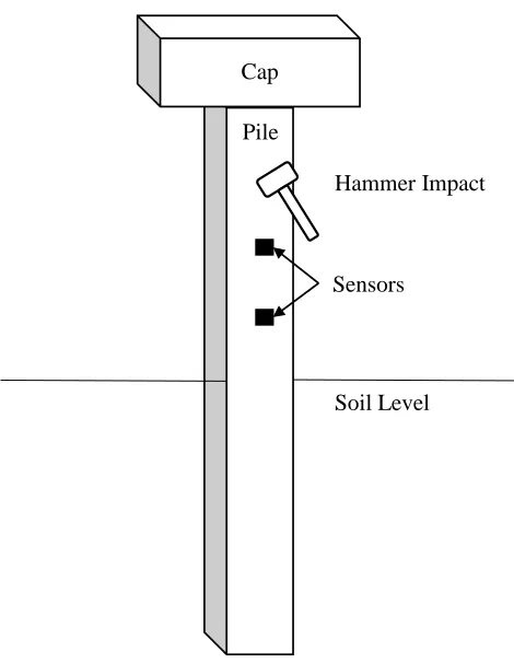
8 response is measured at a minimum of two locations in the foundation using sensors such as accelerometers or geophones. Depending on the location and type of excitation imparted to the pile, several types of waves can exist, such as longitudinal, flexural, and high order guided waves. Figure 2-1 presents a typical pile subjected to lateral impact, which is also the experimental set-up used in this study.
Figure 2-1: Pile and experimental set-up schematic.
We employed EDAR to process responses measured at two sensor locations along the length of a pile. EDAR can be applied for both longitudinal and flexural waves. Similar to the aforementioned surface-based methods, EDAR requires access to the exposed portion of the pile to record accelerations or velocity from a hammer impact at a minimum of two locations along the length of the pile. The major contribution of this paper (and how it differs from earlier methods) is the way the data are processed to estimate the length of a pile. Section 2.3 discusses the concept behind processing the data using the EDAR methodology.
Sensors
Hammer Impact Cap
9 2.3 Effective Dispersion Analysis of Reflections (EDAR): Theory
The fundamental concept of EDAR is based on the difference of individual phases between the responses measured at the two sensor locations. The basic theory is explained for both
longitudinal and flexural waves, followed by verification using synthetic data and validation using laboratory experiments. EDAR presents a unique way to process the same response data that can be obtained from the ultra-seismic or short kernel (bending wave) methods to estimate the length of the pile by incorporating the physical dispersion characteristics of wave
propagation. The phase difference between the responses at the two sensor locations in the frequency domain is given by
2 1
Imag log ( ) log ( )
d
P u u , (2.1)
where u1( ) and u2( ) are the Fourier transforms of the responses (displacements, velocities or accelerations) obtained at the two sensor locations, respectively. The phase difference between the responses obtained at the two sensor locations in the frequency domain contains the product of theoretical wavenumber (k) and the lengths associated with the pile. Generally, the phase depends on the distance the wave has traveled before and after reflections from the various boundaries in the structure. Section 2.3.1 explains the characteristics of the phase difference and extraction of the pile length using simple theoretical models: Section 2.3.1.1 discusses wave propagation without reflections with the help of dispersion analysis, and Section 2.3.1.2 discusses the effects of the reflections and introduces the concept of EDAR plot.
2.3.1 Longitudinal waves in bar 2.3.1.1 Propagation without reflections
10 Figure 2-2: Schematic of infinite bar.
The second order differential equation describing the axial wave propagation in a homogeneous, linear elastic rod with Young’s modulus E and density
is given by2 2
2 2 0
u u
E
x t , (2.2)
which on transformation to frequency domain takes the form
2 2
2 2
2 2 0
b
u u
c
x t , (2.3)
where is the temporal frequency, cb is the bar wave velocity and is given by E , E is Young’s modulus, and
is density. The solution of the equation in frequency domain takes the form( , ) ikx
u x Ae , (2.4)
where k is the wavenumber. The wavenumber can be determined from the frequency by
substituting Equation (2.4) into Equation (2.3), which gives the dispersion relation expressed as Equation (2.5).
b k
c (2.5)
Substituting Equation (2.4) in Equation (2.1) results in the phase difference:
2 1
( )
d
P k L L k L . (2.6)
Thus, the phase difference is a product of the theoretical wavenumber (k) and the distance between the sensors (L). Practically, the phase difference that is calculated from the sensor
x=0 S2 S1
L1
L2
Sensor Locations
ikx i t
11 responses results in wrapping between and . An important aspect of this method is to plot the phase as a function of a newly defined quantity called the ‘effective wavenumber’ (ke), which is the wavenumber scaled by a material constant. Such scaling eliminates the need for the knowledge of material properties in estimating the length in this particular case (as well as in the more complicated case of Bernoulli-Euler beam theory in Section 2.3.2). In the specific case of a bar, because the theoretical wavenumber (k) in Equation (2.5) is directly proportional to the frequency, the effective wavenumber is simply defined as the frequency:
bar e
k . (2.7)
For reasons that will become clear after the reflections are analyzed in Section 2.3.1.2, the plot with the phase difference as the abscissa and the effective wavenumber as the ordinate is called the EDAR plot throughout the rest of the paper. The slope of the EDAR plot is governed by the distance between the sensors (L) and the velocity of the wave propagation (cb):
bar b e d c k P
L . (2.8)
The slope from Equation (2.8) would determine the value on the effective wavenumber axis at which the phase gets wrapped. The value at which the first wrapping occurs is called the cycle period (KI) and is given by
bar b I c K
L . (2.9)
This is the first of the two periods associated with the phase and is a consequence of the initial arrival of the wave. Thus, the cycle is closely related to the time difference between the initial arrivals of the propagating wave at the two sensor locations. As an example, consider a model bar of infinite length with a wave propagation velocity of 1 m/s and lengths L13m and
2 3.5
12
Figure 2-3: Effective dispersion plot for infinite bar: phase difference vs. effective wavenumber.
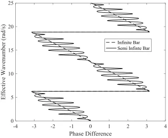
2.3.1.2 Effects of reflections and EDAR plot
Introducing a boundary at x0 makes the bar semi-infinite and results in a single reflection of the wave from the boundary; see Figure 2-4 that assumes a wave traveling from negative infinity towards the boundary where it gets reflected.
Figure 2-4: Semi-infinite bar: single reflection. x=0
S2 S1
L1 L2 Sensor Locations Aeikx i t
ikx i t
13 Without loss of generality, the displacement in the frequency domain anywhere in the bar can be assumed to be
( ) ikx ikx
u x Ae Be , (2.10)
where the first term on the right-hand side represents a forward propagating wave and the second term represents the reflected wave. Similar to the infinite case, a model bar with the same
parameters are considered for a semi-infinite bar, but the displacement form in equation (2.10) is used to account for the reflection from the boundary (reflection coefficient of 0.5) that is
introduced; Figure 2-5 presents the resultant EDAR plot that is computed for a semi-infinite bar. In addition to the cycle oscillations that are similar to those found for the infinite bar, smaller oscillations can be observed with a smaller period in the semi-infinite bar. These small
oscillations, called ‘wiggles’, are a consequence of the wave being reflected at the boundary and can be utilized to estimate the location of the boundary.
14 The responses at the accelerometer locations S1 and S2 at distances L1 andL2, respectively, from the boundary are
1 1
1( )1
ikL ikL
u L Ae Be , (2.11)
2 2
2( 2)
ikL ikL
u L Ae Be . (2.12)
Using these displacements, the phase difference can be calculated from Equation (2.1). The steps involved in calculating the phase difference analytically are shown here as Equations (2.13) through (2.15). 1 2 1 2 2 ( ) 1 2 2 ikL
ik L L ikL
u Ae B
e
u Ae B (2.13)
Taking the logarithm of the ratio shown in Equation (2.13) gives
1 2 2 2 1 2 1 2 ( ) ( ) ( ) ikL ikL u
log ik L L log Ae B log Ae B
u . (2.14)
The imaginary part of Equation (2.14) is the phase difference. The imaginary part of the logarithm of a complex number is the argument of the complex number and thus
1
2 3
1 1 1 2
2 1
1 2
sin(2 ) sin(2 )
( ) tan tan
cos(2 ) cos(2 )
d b b b
A kL A kL
P k L L
B A kL B A kL . (2.15)
The periodic nature of Pd can be explained from the three terms b1, b2, andb3. The first term is exactly the same as the one obtained for the infinite bar and, along with phase wrapping, gives rise to the cycles shown in the EDAR plot in Figure 2-3. The terms b2 and b3 are
responsible for the smaller oscillations or wiggles observed in Figure 2-5. The trigonometric functions b2 and b3 can be shown to have a period of L1 and L2 , respectively. Because the distance between the sensors is small compared to the length of the pile (L1 is approximately equal to L2 that is approximately equal to Le), Le is the distance between the midpoints of the sensors to the boundary. Thus, the period of the last two terms in Equation (2.15) in the
15 bar b R e c K
L . (2.16)
One of the main practical concerns here is obtaining an accurate estimate of the wave velocity for the system under consideration. Often, pile foundations are old and deteriorated and
knowledge about the construction material is hard to obtain. Examining the ratio of the cycle and wiggle periods helps resolve this issue. The ratio of the cycle and wiggle periods is
bar e b I bar e R b c L K L
K c L L . (2.17)
Once the cycle and wiggle periods are calculated from the EDAR plot, the only unknown is lengthLe, which can be computed without need for any other information about the pile. Because the plot effectively captures (a) the effect of the dispersion relation (simple in this case but can be more complicated for beams) and (b) the effect of reflections from the boundary, the plot and the ensuing analysis that result in Equation (2.17) are referred to as the ‘effective dispersion analysis of reflections’, hence, ‘EDAR’.
The proposed EDAR technique is similar to the travel-time approach for nondispersive systems, where the travel time between sensors can be used to compute the wave velocity, which in turn can be used to compute the unknown boundary locations based on the arrival times of the reflections. The key advantage of the proposed EDAR method is that it can be extended to dispersive wave propagation, where travel-time approaches fail due to the significant distortion of the waves that is caused by dispersion. Section 2.3.2 provides details regarding this extension of EDAR.
2.3.2 Flexural waves in beams
Bending waves can be generated by a lateral impact to the pile. The test set-up for bending waves is exactly the same as for longitudinal waves and the responses are likewise measured at a minimum of two sensor locations. There are two main differences between the waves propagating in a bar and a beam. Firstly, along with the propagating waves, there exists evanescent waves, which decay exponentially. Due to this decaying nature, the effect of
16 EDAR processing. Secondly, the propagating waves are dispersive in nature as explained
Equations (2.18) through (2.20) which is a critical for the formulation of the EDAR procedure. The governing differential equation for a homogeneous, linearly elastic Bernoulli-Euler (BE) beam is given by
4 2
4 2 0,
v v
EI A
x t (2.18)
where v is the transverse displacement. Similar to the case for a bar, the general solution for Equation (2.18) can be given by
ikx i t
y e . (2.19)
Substituting Equation (2.19) in Equation (2.18) we get the dispersion relation between wavenumber and temporal frequency given by
b k
c r , (2.20)
where cb is the bar wave velocity and r I A is the radius of gyration. The phase velocity can be calculated from Equation (2.20); clearly frequency-dependent, resulting in wave dispersion, which distorts the waveform as it propagates through the length of the beam. This wave
distortion makes peak-picking difficult and often impossible, thus making travel-time approaches difficult.
The dispersion relation shown in Equation (2.20) is the key to defining the effective wavenumber for EDAR, which is obtained by scaling the wavenumber. Specifically, the material constants and cross-sectional properties are dropped from Equation (2.20) to define the effective wavenumber:
BE e
k . (2.21)
The above choice facilitates the estimation of length without prior knowledge about the material constants, as discussed below. Equation (2.21) also makes the relation between the phase
17 b BE I c r K
L , (2.22)
b BE R e c r K
L . (2.23)
Similarly, taking the ratios of the two periods, a length estimate of the pile (Le) can be obtained as BE e I BE R K L L
K . (2.24)
Once the responses at the sensor locations are obtained, Equation (2.24) requires only the cycle period, wiggle period, and the distance between the sensors to obtain an estimate for the length of the member. The important modification is the definition of the effective wavenumber as the square root of the frequency, thus making the wiggle period constant and facilitating the
extension of the bar length estimation shown in Equation (2.17) to the beam length estimation shown in Equation (2.24).
This method pertains specifically to BE beam theory. BE beam theory is simple, but not accurate for higher frequencies where the wavelength is of the same order as the beam thickness. However, the EDAR methodology can be extended to more sophisticated models, such as
Timoshenko beam theory. The governing equation for a Timoshenko beam with Young’s modulusE, density
, shear modulusG, areaA, moment of inertiaI , and Timoshenko shear coefficient is4 4 2 4
4 2 2 2 4 0
EI y I EI y y I y
A x A GA x t t GA t . (2.25)
The corresponding dispersion relation is
4 2 2 2 4
0
EI I EI I
k k
A A GA GA . (2.26)
18 simplicity of the bar or BE beam model. Different material properties regarding structure might be needed as opposed to not requiring any material properties as is the case with the simpler BE beam model. The EDAR procedure must be used cautiously, paying utmost attention to the frequency content under consideration and the validity of the underlying models. At lower frequencies, use of BE beam theory might be justified, but at higher frequencies, more robust models, such as Timoshenko beam theory or even more sophisticated models based on guided wave theory, may be required.
2.3.3 Synthetic examples for EDAR verification
In this study, a finite BE beam, with square cross section, was modeled with half spaces (HS) on the top and bottom with variable material properties to control the reflection coefficients and to treat reflections from different boundaries separately. Material damping was introduced by using complex values for the modulus of the pile (imaginary part was taken to be 5% of the Young’s modulus). Table 2-1 presents the model BE beam properties and Figure 2-6 presents a schematic of the BE beam model with lengths.
Table 2-1: Model Bernoulli-Euler beam properties. Property Value
Young’s Modulus 35 GPa Density 2400 kg m/s2 Poisson’s Ratio 0.1
Cross section (square)
0.3048 m x 0.3048 m
Figure 2-6: Schematic of Bernoulli-Euler beam model.
A2 A1
1m 0.3m 0.4m 4m
Force
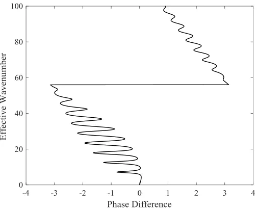
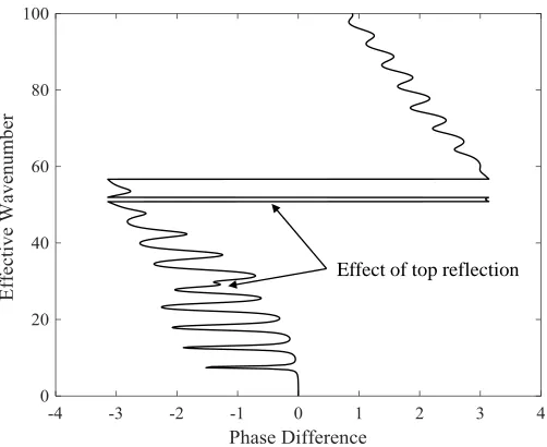
19 Example 1: The top HS is modeled such that it matches the beam to prevent reflections from the top. The bottom HS modulus is a large value to simulate a fixed end. Figure 2-7 presents the EDAR plot obtained from the BE model and Table 2-2 presents the BE model beam length estimates.
Figure 2-7: EDAR plot for synthetic Bernoulli-Euler beam experiment involving bottom reflections.
Table 2-2: Bernoulli-Euler beam model length estimate. Cycle Period Wiggle
Period
Distance between sensors
Estimated Length (m)
Actual Length (m)
Error
64.49 6.2 0.4 5.66 5.7 -0.7%
20 Figure 2-8: EDAR plot for Bernoulli-Euler beam model: bottom and top reflections.
Figure 2-8 shows the effect of the top reflection in the EDAR plot. Even though the top
reflections disturbed the wiggle, the important aspect to note is the distinctive characteristics of the disturbances. They do not look similar to wiggles and can be ignored while calculating the wiggle period. This difference between the disturbances shown and wiggles is a consequence of the impact locations and the wave propagation direction. By using the unaffected wiggles in the EDAR plot, similar length estimates, as shown in Table 2-2, were obtained. Depending on the length to the top of the pile, there can sometimes be interference between the top effect and cycle period. This situation can be avoided by using multiple distances between the sensors, which we did during actual experimentation. We used four sensors instead of the two sensors required for EDAR. In this way, we built redundancy into the test and thus, the cycle and wiggle periods can be obtained from multiple sensor combinations.
2.4 Experimental Validation of EDAR
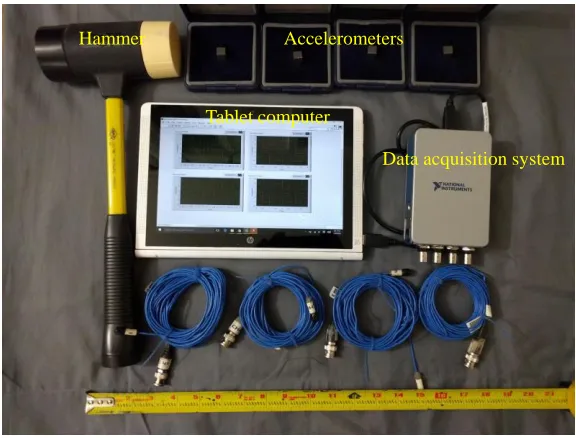
Following the successful verification of EDAR using synthetic data, we performed experiments at the Constructed Facilities Laboratory at North Carolina State University (NCSU) to validate the proposed EDAR. Figure 2-9 shows one of the concrete filled steel tube (CFST)
21 piles, installed as part of a different project at NCSU, which we used for initial testing. Table 2-3 presents the properties of the CFST.
Figure 2-9: Concrete filled steel tube tested at NCSU.
Table 2-3: Properties of concrete filled steel tube.
Property Value (m)
Total Length 5.92 Embedded Length 4.17
Cap Dimensions 0.6096 x 0.4572 x 0.4572 Concrete Diameter 0.292
Steel Thickness 0.0064 Accelerometers
Data acquisition system Hammer
Tablet computer
Impact
S1
S2
S3
22 Accelerometers from PCB (352C33) and a data acquisition system from National Instruments (NI9232) were used respectively for sensing and recording the responses of CFST to a lateral impact from a small sledge-hammer. The impact is applied between the pile cap and top sensor, maintaining sufficient distance from the top sensor to prevent any overload. Figure 2-10 shows the equipment used for laboratory testing and Table 2-4 provides a summary of the equipment specifications.
Figure 2-10: Equipment used for EDAR testing.
Table 2-4: Equipment specifications.
Equipment type Model Important specifications
Item Range
Accelerometer PCB 352C33 Frequency 0 to 10000 Hz
Measurement Range ±50 g Sensitivity 100 mV/g DAQ System NI 9234 with USB
chassis
Analog Input Resolution
24 Bits
Sampling Rate 51.2 KS/s Accelerometers
Data acquisition system Hammer
23 Four accelerometers were used to build redundancy in the data obtained, giving six two-sensor combinations. The distances between the four two-sensors were 0.203, 0.152, and 0.254 m and are directly reflected in the cycle periods observed in the EDAR plots. Figure 2-11 presents the time domain plots of the accelerations obtained at the four sensor locations. Examining these time histories indicates that there are no clear peaks associated with incident and reflected waves, owing to the dispersion associated with flexural waves.
Figure 2-11: Experimental response: time domain.
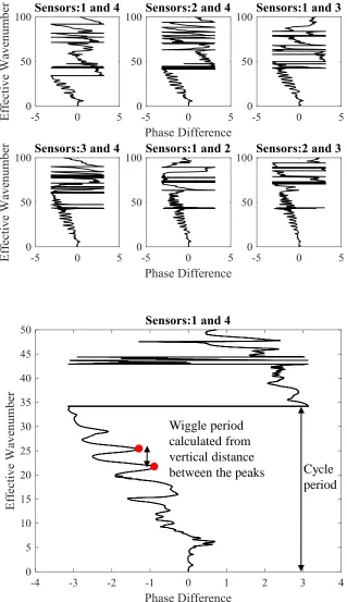
24 Figure 2-12: (a) Representative experimental EDAR plots (b) Finding wiggle and cycle period
from EDAR plot.
Cycle period Wiggle period
25 Figure 2-13: Theoretical dispersion relation: Bernoulli-Euler vs. Timoshenko beam theories.
It is well known that Timoshenko beam theory is more accurate than BE theory for higher frequencies, but at low frequencies the dispersion curves overlap for both models. Thus, using the lowermost wiggle in the frequency axis and cycle period between the farthest two sensors, a length estimate can be obtained.
Table 2-5: Length estimate from first observed wiggle using Bernoulli-Euler beam theory. Cycle period Wiggle
period from lowermost
wiggle
Distance between sensors
Estimated length (m)
Actual length (m)
Error
34.18 3.63 .6096 5.74 5.92 3%
26 wavenumber axis. Each of these wiggles were used to calculate the wiggle period and
subsequently used to estimate the length. As explained earlier, the main difference between the BE and Timoshenko beam theories is the theoretical wavenumber axis, and thus, the cycle and wiggle periods are changed, as shown in Figure 2-14. In Figure 2-15, the length estimates obtained from each observed wiggle are plotted as a function of the frequency at each wiggle. Clearly, the BE beam theory estimates are a function of the frequency and increase as we move up the frequency. This frequency dependence is reduced greatly for estimates obtained using Timoshenko beam theory, and the average error percentage also is reduced significantly (see Table 2-6).
Figure 2-14: Comparison of Bernoulli-Euler and Timoshenko EDAR plots. BE
I K
Timo I K
Timo R K
27 Figure 2-15: Length estimates as a function of frequency.
Table 2-6: Average length estimates. Bernoulli-Euler
theory
Timoshenko theory Actual length (m)
Estimate (m) 6.69 5.99 5.92
Error 13% 1.18%
Unlike Timoshenko beam theory, BE beam theory does not require any information about the pile properties to calculate the effective wavenumber defined in Equation (2.21). However, BE theory leads to a less accurate representation of the exact physical system, and thus, the resulting estimates are less accurate. Therefore, depending on the availability of material property
estimates and location of the wiggles in the frequency axis, one of the two theories can be used to obtain the length.
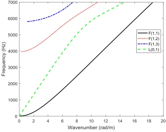
28 research efforts conducted at Northwestern University by Finno [39], Hanifah [40], Chao [41], Wang [42], and Lynch [43] have considered the pile as a cylindrical wave guide to obtain the longitudinal, torsional, and flexural modes of vibrations and corresponding dispersion relation. The predominant modes in longitudinal and flexural waves are the first modes, namely L(0,1) and F(1,1), for frequencies excited via hammer impact, which gives us more confidence to use a 1-D wave propagation model.
2.5 Conclusion
A newly developed NDE methodology, EDAR, is introduced in this work. EDAR is based on obtaining the phase difference of responses at two different locations on a pile in the frequency domain as a function of a newly defined quantity called the ‘effective wavenumber’. The effective wavenumber is a function of the dispersion relation of the model chosen to represent the physical system and the type of impact. The theory behind EDAR is based on longitudinal and flexural waves. We conducted experimental validation and found the pile length estimates to be consistently within a 5 percent error margin. EDAR methodology is based on the underlying physics of wave propagation and thus improves reliability for the results obtained. EDAR is currently being evaluated in the field, following its success in laboratory test
29 Chapter 3
Nondestructive Length Evaluation of an Embedded Pile Using Lateral Hammer Impact: Combined Transverse and Longitudinal Waves
Abstract
This paper presents an important modification of the recently developed nondestructive testing method for estimating embedded depth of pile foundations – EDAR – effective dispersion analysis of reflections. The original EDAR method is based on processing dispersive bending wave signals in the frequency-effective wavenumber domain, thus eliminating the need to perform peak picking that is difficult due to over-distortion of reflected signals. While the method was successful in laboratory settings, preliminary field validation resulted in significant errors. After careful examination of the wave physics, it is discovered that both longitudinal and transverse waves need to be carefully included in EDAR analysis. Specifically, it is shown that the initial arrival is dominated by transverse waves, while the reflections are dominated by longitudinal waves, owing to significant attenuation of transverse waves due to compacted soil around the pile. This observation led to a refined EDAR methodology and accurate estimation of embedded pile depth in field settings.
3.1 Introduction
Missing records of bridges has been a longstanding issue and systemic problem in USA. Engineers have relied on several nondestructive evaluation techniques to obtain the crucial length information about bridge pile foundations, especially when they are classified as scour critical. There are still about 28,000 highway bridges with unknown foundations in 2016 that could be potentially susceptible to scour according to National bridge inventory. Several other bridges over land are also expected to have unknown foundation and missing or incomplete records [2]. Thus, there is a need for an easy and effective nondestructive methodology to estimate the length of pile foundations.
30 often expensive and time-consuming due to the need for a borehole near the foundation. In contrast, surface-based methods rely on generating waves through an impact and recording the response at specific sensor locations. Testing is easier, but these methods do not provide the same level of reliability as borehole methods. Surface-based methods for length estimation purposes mainly include sonic echo, impulse response, ultraseismic and bending wave
techniques. This paper discusses a newly developed methodology that utilizes multiple types of waves generated through a hammer impact.
One of the most widely used method for length estimation is the sonic echo or pulse echo method which involves impacting pile top leading to generation of longitudinal waves. This method has been standardized by ASTM (D5882-16) and several researchers have used this methodology in a variety of situations over the years (e.g., [9], [12], [37]). These waves are non-dispersive in nature i.e. all the frequencies travel at the same velocity. Thus, there is minimal distortion of the initial waveform in the time domain and peak picking can help determine the distance of wave propagation. This has been very successful for newly constructed bridges both for length estimation and integrity evaluations but has limitations for existing bridges due to reduced access to the top of the pile. Researchers have tried various methods to induce
longitudinal waves without access to the top, but the recorded waveforms tend to be complicated to be able to process. Existing piles have much easier access to the sides of the piles and
producing a lateral impact leading to flexural or bending waves is easier from the experimental and site perspective. Using lateral excitations for pile length estimation was introduced by Holt and Douglas [16]. Unlike longitudinal waves, flexural waves are dispersive in nature and thus distort as they propagate making any time domain processing of the signals complicated. In order to analyze these complicated signals, the bending wave or short kernel method was introduced. This method helps obtain travel-time information through convolution of the signal with a chosen kernel of specific frequency. The choice of kernel frequency and peak picking is still complicated even for experienced users leading to higher error percentages [22]. Other methods based on signal processing techniques have also been investigated (e.g., [21], [23]). Major drawback of these methods is that they are purely signal processing based methods and do not explicitly incorporate the underlying physics that causes wave distortion.
31 difference between the responses obtained at two accelerometer locations, due to an impact applied to the side of the pile, as a function of a newly defined quantity called the effective wavenumber. Effective wavenumber is defined based on the physical dispersion of the wave generated from impact. Given this general definition of effective wavenumber, EDAR can be easily applied to both longitudinal and flexural waves. EDAR methodology was initially tested in the laboratory resulting in length estimates with errors less than 5% and its extension to a field piles is presented in this paper. In contrast with the success in the lab, preliminary application of EDAR for field data indicated significant underestimation of the embedded pile depth. A closer look at the physics of waves indicated that there is a significant effect of the compacted soil found in the field, necessitating a revision of the original EDAR methodology. Specifically, it is observed that the compacted soil causes differential attention of longitudinal and transverse waves. This paper is focused on a detailed discussion of the phenomenon, and a resulting modification to EDAR methodology that results in accurate estimation of embedded pile depths in field settings.
The outline of the paper is outlined as follows. Section 3.2 contains a brief introduction to the original EDAR methodology and a summary of laboratory validation. Preliminary length estimates obtained from direct application of EDAR to field data are presented Section 0. Section 3.4 contains the reasons for discrepancies in the initial length estimates, while Section 3.5
contains the modified EDAR methodology for compacted soils. The paper is concluded with field validation in Section 3.6, followed by concluding remarks in Section 3.7.
3.2 EDAR Preliminaries
Traditionally surface-based techniques have relied on generating a wave through a hammer strike at various locations on the exposed parts of the pile. The main two types of waves that are generated are the longitudinal and flexural/transverse waves. Depending on the type of hammer impact and the sensor orientation various waves can be recorded (Figure 3-1).
32 Effective Dispersion Analysis of Reflections (EDAR), which has the potential to analyze both longitudinal and flexural waves with equal ease to obtain length information from the pile response.
Figure 3-1: Pile setup (a) Top impact (b) Side impact.
3.2.1 Theory
EDAR requires a minimum of two sensors along the length of the exposed region of the pile either capable of measuring lateral or longitudinal accelerations. The impact should be above the top sensor and could be in either longitudinal or lateral direction. The phase difference (Pd) is defined by,
2 1
Imag log ( ) log ( )
d
P u u , (3.1)
where u1 and u2 are the frequency-domain representation of responses (accelerations, velocities or displacements) at the two sensor locations. We introduce the concept of effective
Sensors (measuring lateral acceleration) Hammer Impact – Side Cap
Soil Level Pile
Hammer Impact – Top
Pile
(a) (b)
33 wavenumber, which is essentially a scaled wavenumber and is based on the dispersion relation of the propagating waves. For longitudinal waves, the wavenumber (k) and have a linear
relationship with the bar wave velocity (Cb) as the proportionality constant:
b k
c . (3.2)
Correspondingly, effective wavenumber is defined as,
e
k , (3.3)
which is proportional to the wavenumber but is independent of the wave velocity. This specific definition facilitates the estimation of the pile length without the need for the material properties of the pile, as explained below. The general form of wave propagating in a bar is given by,
( ) ikx ikx
u x Ae Be . (3.4)
Using the Equations (3.1) and (3.4), the phase difference can be derived as [44],
1 1 1 2
2 1
1 2
sin(2 ) sin(2 )
( ) tan tan
cos(2 ) cos(2 )
d L
A kL A kL
P k L L
B A kL B A kL . (3.5)
d
P is periodic in nature with two periodicities, defined as cycles and wiggles. The first term is the theoretical wavenumber scaled by the distance between the sensors (L ) which along with phase wrapping leads to cycle period as shown in Figure 3-2. The second and third term are responsible for the smaller oscillations called wiggles observed in Figure 3-2. The trigonometric functions have periods
L1 and
L2which can be approximated to
Le, where Le is the distance from midpoint of the sensors to the tip of the pile. A semi-infinite bar with lengths L1=3m, L2=3.5 m as shown in Figure 3-1 and velocity of wave propagation c=1 m/s was simulated
34 Figure 3-2: EDAR plots for Semi-Infinite bar with characteristic cycle and wiggle periods.
The cycle and wiggle periods shown in Figure 3-2 is given respectively by
bar b I
c K
L , (3.6)
bar b
R e
c K
L . (3.7)
The ratio of the cycle and wiggle periods is
bar e I
bar R
K L
K L. (3.8)
Once the cycle and wiggle periods are obtained from the EDAR plot, the only unknown in equation (3.8) is e
L can be calculated giving us an estimate of the pile length. This is very similar to travel-time approaches where the velocity of wave propagation is calculated based on travel time between sensors and pile length calculated from the travel time of the reflected wave. In addition to providing an easier and alternate analysis methodology for processing
non-dispersive waves, the key advantage of EDAR is that it can be extended to non-dispersive waves in a beam, where the travel time approach fails due to significant distortion in the waves. Similar to the bar, the dispersion relation of a Bernoulli-Euler (BE) beam is given by
Wiggle
35
b k
c r (3.9)
where r I A is the radius of gyration. The phase velocity is frequency-dependent, resulting in wave dispersion, i.e. distortion the waveform as it propagates through the length of the beam. We correspondingly define the effective wavenumber as the quantity proportional to the
wavenumber but independent of the material and section properties:
BE e
k , (3.10)
The above makes the relationship between phase difference and effective wavenumber linear and all the results described earlier for the bar can be directly applied to the BE beam. The length estimate of the pile can derived based on Equation (3.8) adapted to Bernoulli-Euler beam:
BE e I BE R K L L
K . (3.11)
More sophisticated models can be used in place of B-E beam theory to more accurately represent the waves propagating in the piles. For example, theoretical wavenumber obtained from
Timoshenko beam theory can be used as effective wavenumber to obtain the EDAR plot which modifies both the cycle and wiggle periods leading to an improved length estimate. The key in selecting the appropriate definition for effective wavenumber lies in carefully examining the type of waves and the range of frequencies in which the cycle and wiggle periods occur. If the
propagating waves are predominantly longitudinal in nature, simple bar model can be used. If the waves are predominantly transverse in nature and wavelengths are significantly higher than the cross-sectional dimensions, use of BE beam theory can be justified (since the slenderness ratio would be large). Otherwise, the Timoshenko beam theory or even more sophisticated guided wave modelling may be needed to obtain accurate length estimates.
3.2.2 Laboratory testing
36 acceleration of the foundation. Large sledge hammer (PCB 086D50) with hard and soft tips and a small sledge hammer (0.45 Kg) with hard, medium hard, medium and tough tips were chosen to impact the piles in between the cap and top sensor. The results for the hard tip of the large and small sledge hammers are presented here for the laboratory tests.
EDAR methodology was validated in laboratory testing using concrete filled steel tubes (CFST). The properties of CFST and other details of the laboratory test can be found in
references [44] and [38]. Total length of the pile was 6.33 m with 4.22 m embedment. The concrete diameter was 0.292 m with a steel thickness of 0.00635 m. Four sensors, numbered one to four from top to bottom, were used with spacing of 0.2, 0.16, and 0.25 m. The distance from the midpoint of the sensors to the bottom of the cap is 1.1 m. Typical EDAR plot for two pairs of sensors are shown in Figure 3-3. The data shown in the time domain on the left does not
immediately provide much information. On the other hand, the EDAR plots on the right clearly show cycles and wiggles, which can be used to estimate the embedded depth, as described below.
The periodicities explained earlier can be clearly seen in the EDAR plots for which the effective wavenumber was obtained using Equation (3.10). The data were analyzed using Timoshenko beam theory. The dispersion relation for Timoshenko beam with Young’s modulus
E, density
, shear modulusG, areaA, moment of inertiaI , and Timoshenko shear coefficient , is given by:4 2 2 2 4
0
EI I EI I
k k
A A GA GA (3.12)
The Timoshenko shear coefficient for a rectangular section can be obtained using [45], 10(1 ) 12 11
(3.13)
37 Figure 3-3: Laboratory pile (a) Time history at accelerometers 1 and 4 (b) Time history at
accelerometers 2 and 3 (c) Representative EDAR plots.
Figure 3-4: Wiggle period as a function of frequency for large (LH) and small (SH) sledge hammers hard tip.
(a)
(b) (c)
0 1 2 3 4 5 6 7 8 9
0 1000 2000 3000 4000 5000
L
eng
th
Esti
mate
s (m)
Frequency (Hz)
38 Lower frequency estimates had lesser errors and it can be seen that the scatter gets bigger as we go higher up the frequency. Nevertheless, the overall trend of the estimates is fairly flat giving us a good average length estimate as shown in Table 3-1. Although there was not much variation between the results obtained from different hammer tips in the laboratory tests, hammer type and tip played an important role in the results obtained in the field as presented later.
Table 3-1: Length Estimates for laboratory pile. Actual
Length
Frequency Range
SH LH
Average Estimate (m)
Error Average Estimate (m)
Error
6.33 <1500 Hz 6.52 3 % 6.46 2.1 %
>1500 Hz 6.75 6.6 % 6.85 8.2 %
All 6.67 5.4 % 6.61 4.4 %
3.3 Observations from Field Testing
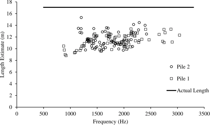
39 Table 3-2: Field pile properties.
Property Value
Design concrete compressive strength (Fc’) 68.9 MPa Estimated modulus (using AASHTO 5.4.2.4-3) 41.8 GPa
Cross section – square 0.4064 m
Total length 17.07 m
Top of pile to bottom-most sensor (pile 1) 1.74 m Top of pile to bottom-most sensor (pile 2) 2.4 m
Figure 3-5: (a) Field piles (b) Equipment and sensor location.
Material properties to calculate the Timoshenko wavenumber are in general not readily available in case of unknown foundations. In this particular case though design strength is available from design drawing and used to obtain the initial estimates (a more robust procedure to obtain the material properties is outlined in Section 3.6.1). The density of concrete was
assumed to be 2,400 Kg/m3 and Young’s modulus value was calculated as 41.8 GPa from the 28-day design compressive strength using AASHTO LRFD equation 5.4.2.4-3. Poisson’s ratio of concrete is typically between 0.1 to 0.2 and is assumed to be 0.15 for this part of the analysis. Length estimates are obtained by analyzing the data obtained in the field using the same
Pile #1
Pile #2
Sensor Location