R E S E A R C H
Open Access
On a general filter regularization method for
the 2D and 3D Poisson equation in physical
geodesy
Nguyen Huy Tuan
1*, Binh Thanh Tran
2and Le Dinh Long
3*Correspondence:
[email protected]; [email protected]
1Faculty of Mathematics and
Statistics, Ton Duc Thang University, Ho Chi Minh City, Vietnam Full list of author information is available at the end of the article
Abstract
In this paper, we consider a Cauchy problem for the Poisson equation with nonhomogeneous source. The problem is shown to be ill-posed as the solution exhibits unstable dependence on the given data function. Using a new method, we regularize the given problem and obtain some new results. Two numerical examples are given to illustrate the effectiveness of our method.
MSC: 35K05; 35K99; 47J06; 47H10
Keywords: Poisson equation; Cauchy problem; ill-posed problem; convergence estimates
1 Introduction
The Poisson equation is
u=f, ()
whereis the Laplace operator,f anduare real or complex-valued functions on a mani-fold.
In case off = , equation () is called Laplace’s equation which arises naturally in many areas of engineering and science, especially in wave propagation and vibration phenom-ena such as the vibration of a structure [], the acoustic cavity problem [], the radiation wave [] and the scattering of a wave []. For example, certain problems related to the search for mineral resources, which involve interpretation of the earth’s gravitational and magnetic fields, are equivalent to the Cauchy problem for Laplace’s equation. In another application of geophysical underground prospection, the geoelectrical method has been initiated in recent years (see the historical account in Zhdanov and Keller []). In fact, by now the geoelectrical method involves, even in its most basic formulation, the solution of the Cauchy problem for Laplace’s equation.
Nowadays, the Cauchy problem for Laplace’s equation, and more generally for ellip-tic equations, has a central position in all inverse boundary value problems which rep-resent electrical impedance tomography, optical tomography and transient phenomenon in a time-like variable, while elliptic equations describe steady-state processes in physical fields.
In physics, a gravitational field is a model used to explain the influence that a massive body extends into the space around itself, producing a force on another massive body. Therefore, a gravitational field characterizes gravitational phenomena and is measured in Newtons per kilogram (N/kg). In its original concept, gravity was a force between point masses. Following Newton, Laplace attempted to model gravity as some kind of radiation field or fluid, although the th century explanations of gravity have usually been sought in terms of a field model rather than a point attraction. A gravitational field is the force field created around massive bodies that causes attraction of other massive bodies. A dis-tribution of matter of densityρ=ρ(x,y,z) gives rise to a gravitational potentialφ which satisfies the three-dimensional (D) Poisson equation
φ= –πGρ ()
at the points inside the distribution, whereGis the universal gravitational constant. Motivated by important applications of the Poisson equation, in this paper we are in-terested in considering the Cauchy problem of identification of the gravitational fieldφ
which satisfies a Poisson equation (two-dimensional case or three-dimensional case). As first pointed out by Hadamard, the Cauchy problem for Laplace’s equation is an ill-posed problem. It means the problem’s solutions do not always exist and, whenever they do exist, there is no continuous dependence on the given data. A small perturbation in the Cauchy data therefore can affect the solution significantly. Readers are referred to [–, –] for earlier materials on the Cauchy problem for Laplace’s equation. For the homogeneous case of source term, the elliptic problem was considered in a series of articles analyzing the sta-bility and convergence (see,e.g., [–, , , ]). A similar version of Laplace’s equation with homogeneous case was considered by Regińskaet al.[, ], Lesnicet al.[], Taut-enhahn [] and Weiet al.[–].
Although we have many works on the homogeneous case of the elliptic problem, the lit-erature on the inhomogeneous case, for example, the Poisson equation, is quite scarce. The earlier work on the abstract elliptic second order equation with inhomogeneous source was introduced in [] by Showalter (see p.). The main aim of this paper is to present a general regularization method and investigate the error estimate between the regular-ized solution and the exact solution.
Our paper is organized as follows. In Sections and , we construct stable approximate solutions of the equation and give the convergence estimates for D and D cases, respec-tively. Finally, in Section , two numerical examples for each D and D case are devised to test the effectiveness of proposed methods.
2 The 2D case of the Poisson equation 2.1 Mathematical model
We consider the problem of findingφ(x,y) such that
φ=φxx+φyy=f(x,y), (x,y)∈×(, ) ()
subject to the boundary conditionφ(x,y) = ,x∈∂. Here= (,π) andϕ,g∈L(,π)
L(, ;L(,π)). Let{u
we have the following system:
φp(y) +λpφp(y) =fp(y),
Hence, we obtain the solution of Problem () as follows:
φ(x,y) =
From (), we see that the data error can be arbitrarily amplified by the ‘kernel’ function cosh(py). That is the reason why equation () is ill-posed in the sense of Hadamard. In the paper of Hadamard, he provided a fundamental example which shows that a solution of a Cauchy problem for Laplace’s equation does not depend continuously on the data. The example is as follows:
u= , (x,y)∈R,y> , ()
uy(x, ) =Ansinnx, x∈R. ()
2.2 A general filter regularization method
To find some regularized solutions, we should replace ‘instability’ kernels cosh(py), sinh(py),sinh(p(y–s)) by the ‘stability’ kernelsA(β,p,y),B(β,p,y),C(β,p,y) that satisfy
and some suitable conditions which are given later. Following property (P), one can
con-struct other kernels. Furthermore, the idea of the above property can be applied to other ill-posed problems such as,e.g., the backward heat conduction problem [].
Throughout this section, we assume that the functionsϕ,g∈L(,π) andf ∈L(, ;
L(,π)). In reality, they can only be measured with some measurement errors, and we
would actually have noisy data:
ϕ(x) =
Here the constant> represents a bound on the measurement error and · denotes the norm inL(). As noted above, we present the following general regularized solution:
Theorem (A general regularization method) Assume thatφ(x,y)is the exact solution of Problem()and Mis a real-valued function such that
∞
Proof The proof will be split into two parts as follows. Part . We estimate φ–v , wherev is defined as
By a simple calculation, we get
+
From (), the partial derivative ofφwith respect toyis
φy(x,y) =
Combining () and (), we obtain
Combining () and (), we have
φ(·,y) –φ(·,y)≤φ(·,y) –v(·,y)+φ(·,y) –v(·,y)
≤
M
(β) + +M(β)E. ()
This completes the proof.
Proof First, we find the functionsM,M,Msuch thatP(β,p,y) holds (), (). Using
β. The admissible regularization parameter is
β=
Applying Theorem , we obtain
On the other hand, for ≤y≤, we have
. Next, we prove that this regularization
param-eterβ=k( <k< ) is admissible by checking condition (). In fact,
Applying Theorem , we obtain
φ–φ≤
3 The 3D Poisson equation
Letρbe the given mass density. For simplification, we consider the problem: determine the gravitational potentialφsuch that the Poisson equation
φ(x,y,z) = –πGρ(x,y,z) ()
subject to the homogeneous Dirichlet boundary conditionφ(x,y,z) = , (x,y)∈∂,z∈ (, ), where= (,π)×(,π). The data ofφatz= :φ(x,y, ) =ϕ(x,y) andφz(x,y, ) =
By a similar way as in (), we find the solution of () that
Physically,ϕcan only be measured with some measurement errors, and we would actu-ally have a disturbed data function
ϕ(x,y) =
where the constant> represents a bound on the measurement error, · denotes the L-norm.
where E is a positive number.Let P(β,p,q,z)be a function such that for anyβ> ,there exist functions N(β)and N(β)satisfying
(a) –P(β,p,q,z)≤N(β)N(p,q), ()
(b) P(β,p,q,z)≤N(β)e–z
√
p+q
, ()
thenφ(x,y,z)defined by equation()fulfills the following estimate:
φ–φ≤
N
(β) + +N(β)E. ()
A choiceβ=β()is admissible if
lim
→β() =lim→N(β) =lim→N(β) = . ()
Theorem Let P(β,p,q,z) = e–z
√
p+q
β(√p+q)m+e–z√p+q for m≥.Assume thatφis the exact solution of Problem()such that
∞
p=
p+qm/φ(x,y,z),sinpxsinqy+ p+qm–φz(x,y,z),sinpxsinqy
≤E ()
for z∈[, ].If we selectβ=k( <k< ),then
φ–φ≤ E
kln()+
√
+ –k. ()
Proof First, we find the functionsN,N,N such thatP(β,p,q,z) holds (), (). We
have
–P(β,p,q,z) = – e
–z√p+q
β(p+q)m+e–z√p+q =
β(p+q)m
β(p+q)m+e–√p+qz. On the other hand, for ≤z≤, we have
β(p+q)m+e–√p+qz ≤
β(p+q)m+e–√p+q. Now, we prove that
β(p+q)m+e–√p+q ≤ mm
βlnm(mβ).
In fact, let the functionhbe defined byh(x) =β
xm+e–Mx. By taking the derivative ofh, one has
h(x) = βmx
m––Me–Mx
The equationh(x) = gives a unique solutionxsuch thatβmxm––Me–Mx= . It means
Using this inequality forM= , we have
–P(β,p,q,z)≤ m Applying Theorem , we obtain
4 Numerical experiment
In this section, simple examples for the D and D Poisson equations are devised for ver-ifying the validity of our proposed methods.
4.1 Example 1
Consider the D Poisson equation as follows:
⎧ ⎪ ⎨ ⎪ ⎩
φxx+φyy=f(x,y), (x,y)∈(,π)×(, ),
φ(x, ) =ϕ(x), x∈(,π),
φy(x, ) =g(x), x∈(,π),
()
where
ϕ(x) = ,
f(x,y) = x+ y–π– e–x+ysin(x)sin(πy)
– πy+πe–(x+y)sin(x)cos(πy)
– xe–(x+y)cos(x)sin(πy)
+e–(x+y)sin(x)sin(πy) y– x– π–
–e–(x+y)sin(x)cos(πy)yπ+ π
– xe–(x+y)cos(x)sin(πy),
g(x) =πe(–x)sin(x) + πe–xsin(x).
Problem () has a unique solution as follows:
φ(x,y) =ex+ysin(x)sin(πy) +e–(x+y)sin(x)sin(πy).
Now we are seeking a solution of the following problem:
⎧ ⎪ ⎨ ⎪ ⎩
φ
xx+φyy=f(x,y), (x,y)∈(,π)×(, ),
φ(x, ) =ϕ(x), x∈(,π),
φy(x, ) =g(x), x∈(,π).
()
We assumehto be a measured data as follows:
h(x) = p
p=
hp+rand(p)
sin(px),
wherep≤p∞and{rand(·)}is an array of pseudo-random numbers satisfying
p
p=
Let (p,p∞) satisfy
O h :=
p∞
p=p+
|fp|≤. ()
In this paper, we choosep= ,p∞= , then () is satisfied.
Step . ChooseLandK to generate the temporal and spatial discretization in such a manner that
xi=ix, x=
π
K,i= , . . . ,K,
yj=jy, y=
L,j= , . . . ,L.
Of course, the higher value ofKandLwill provide more accurate and stable numerical results; however, in the following numerical examplesK=L= are satisfied.
Step . We choose the following functions:
ϕ=ϕ+∗rand( ), g=g+∗rand( ), f=f +∗rand( , ).
Step . Setφβ(xi) =φβ,jandφ(xj) =φj, construct two vectors containing all discrete val-ues ofφ
βandf denoted byβand, respectively,
β=φβ, φβ, · · · φβ,K∈RK+,
= [φ φ · · · φK– φK]∈RK+.
Step . Error estimate between the exact solutions and regularized solutions. At a fixed pointy∗, the error estimationδi, inL
between the exact solutionφand the regularized
solutionsφi,is given by the following formula. Relative error estimation:
δ=
K
i=|φβ(xi) –φ(xi)|L(,π)
K
i=|φ(xi)|L(,π) .
In one example, we have the first regularized solution (defined in Theorem ). In method two, we have the second regularized solution (defined in Theorem ). With parameter
k= /, in the first method we chooseβ= –
ln, and in the second method we choose
β=/.
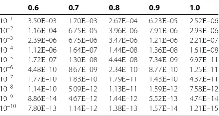
Tables and show the computed error estimations δ at each fixed value y=j/, j= , . . . , . The errors are significantly small when≤–. Comparing the errors of two
Table 1 Discrete relative error estimations for the regularized solution at fixed values from y= 0.0 toy= 0.5
0.0 0.1 0.2 0.3 0.4 0.5
10–1 5.10E–03 2.10E–03 5.60E–03 4.70E–03 7.19E–04 3.40E–03 10–2 2.92E–05 3.16E–04 1.89E–04 6.91E–05 1.33E–04 3.72E–04 10–3 4.30E–07 1.76E–05 6.78E–05 2.31E–05 2.14E–06 2.24E–05 10–4 1.45E–06 6.35E–07 1.02E–06 3.51E–07 1.34E–07 1.28E–06 10–5 1.13E–07 2.82E–09 2.04E–07 5.61E–08 1.05E–07 1.81E–07 10–6 1.83E–08 1.95E–08 3.93E–08 1.24E–08 1.23E–08 1.07E–08 10–7 1.36E–09 4.41E–09 7.11E–10 7.04E–10 9.19E–10 7.78E–10 10–8 1.60E–11 1.69E–10 2.74E–10 2.92E–10 2.18E–10 9.72E–11 10–9 9.04E–12 1.08E–11 1.83E–12 3.84E–12 7.57E–12 1.40E–11 10–10 2.39E–13 1.63E–12 6.78E–12 3.14E–13 6.54E–12 2.35E–12
Table 2 Discrete relative error estimations for the regularized solution at fixed values from y= 0.6 toy= 1.0
0.6 0.7 0.8 0.9 1.0
10–1 3.50E–03 1.70E–03 2.67E–04 6.23E–05 2.52E–06 10–2 1.16E–04 6.75E–05 3.96E–06 7.91E–06 2.93E–06 10–3 2.39E–06 6.75E–06 3.47E–06 1.21E–06 2.21E–07 10–4 1.12E–06 1.64E–07 1.44E–08 1.36E–08 1.61E–08 10–5 1.72E–07 1.30E–08 4.44E–08 7.34E–09 9.97E–11 10–6 4.48E–10 8.67E–09 2.34E–10 8.77E–10 1.25E–11 10–7 1.77E–10 1.83E–10 1.79E–11 1.43E–10 4.37E–11 10–8 1.14E–10 5.09E–12 1.13E–11 1.59E–12 7.58E–12 10–9 8.86E–14 4.67E–12 1.44E–12 5.52E–13 4.74E–14 10–10 7.80E–13 1.14E–12 1.38E–13 1.57E–14 1.21E–15
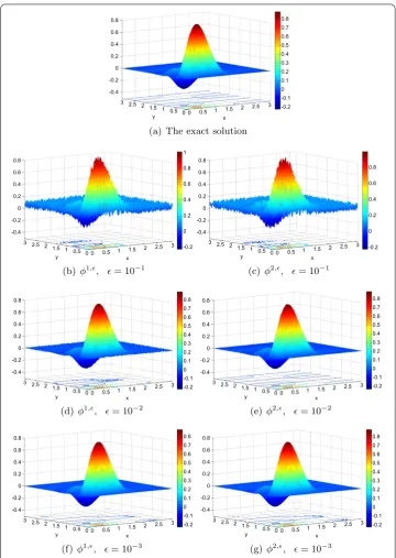
of better illustration, we also present some graphical figures. Figure is the D represen-tation of the exact solution and regularized solutions when= –,= –and= –.
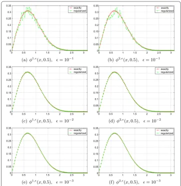
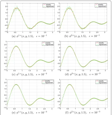
Figure shows graphs of section cut of these solutions at valuey= . when = –,
= –and= –. It is easy to see that our methods are stably convergent.
4.2 Example 2
We consider the following D problem:
⎧ ⎪ ⎪ ⎪ ⎨ ⎪ ⎪ ⎪ ⎩
φxx+φyy+φzz=f(x,y,z), (x,y,z)∈×(, ),
φ(x,y,z) = , (x,y)∈∂,
φ(x,y, ) =ϕ(x,y),
φz(x,y, ) =g(x,y),
()
where= (,π)×(,π).
Step . ChooseQandK(in our computations,Q=K= are chosen) to have
xi=ix, x=
π
Q,j= ,Q,
yj=jy, y=
π
K,i= ,K,
zk=kz, z=
Figure 1 3D graphs of the exact solutionφ(x,y) and three regularized solutionsφi,(x,y) ati= 1, 2.
Step . We choose the following functions and fixz,
ϕ=ϕ+rand(·,·), g=g+rand(·,·),
Figure 2 Section cut of the exact solution and regularized solutions aty= 0.5,= 10–1,= 10–2,
= 10–3.
Step . In this example, we fixz. We putφ(·,·,z∗)β()(xi,yj) =φ(·,·)β(),i,jandφ(·,·,z∗)(xi,
yj) =ui,j, construct two vectors containing all discrete values ofφ(·,·)βandφ(·,·) denoted byβand, respectively,
β()= ⎡ ⎢ ⎢ ⎢ ⎢ ⎢ ⎢ ⎢ ⎣
φ(,,)β(), φ(,,)β(), · · · φ(,,β(),K–) φ(,,β(),K) φ(,,)β(), φ(,,)β(), · · · φ(,,β(),K–) φ(,,β(),K) φ(,,)β(), φ(,,)β(), · · · φ(,,β(),K–) φβ(,,(),K)
· · · . .. · · · ·
φ(,β(Q),,) φ(,β(Q),,) · · · φ(,β(Q),,K–) φ(,β(Q),,K)
⎤ ⎥ ⎥ ⎥ ⎥ ⎥ ⎥ ⎥ ⎦
∈RK+×RQ+,
= ⎡ ⎢ ⎢ ⎢ ⎢ ⎢ ⎢ ⎢ ⎣
φ(,) φ(,) · · · φ(,K–) φ(,K) φ(,) φ(,) · · · φ(,K–) φ(,K) φ(,) φ(,) · · · φ(,K–) φ(,K)
· · · . .. · · · ·
φ(Q,) φ(Q,) · · · φ(Q,K–) φ(Q,K)
⎤ ⎥ ⎥ ⎥ ⎥ ⎥ ⎥ ⎥ ⎦
Step . The error estimation.
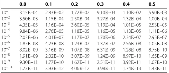
Table 3 Discrete relative error estimations for the regularized solution at fixed values y=π/12 andz= 1.5 fromy= 0.0 toy= 0.5
Now we are seeking a solution of the following problem:
⎧ ⎪ ⎨ ⎪ ⎩
φxx +φyy+φzz=f(x,y,z), (x,y)∈(,π)×(, ),
φ(x,y, ) =ϕ(x,y), x∈(,π),
φ
y(x,y, ) =g(x,y), x∈(,π).
()
Due to the computational cost, we only computed the value of regularized solution
φ(x,y,z) at the fixed valuesy∗=π/ andz∗= .. The discrete relative error estimation in one dimension is defined as follows:
δ y∗,z∗=
p
i=|φp(xi,y∗,z∗) –φ(xi,y∗,z∗)|
i=|φ(xi,y∗,z∗)|
()
with N= being the grid size alongx axis. The regularized solution is calculated by formula () and Theorem with parameterβ=. Computational results are shown in Tables and (the relative error) and in Figure (section cut graphs). In this problem, the
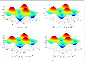
Figure 4 3D graphs ofϕ(x,y) and three regularized solutionsϕi,(x,y).
Figure 5 3D graphs ofg(x,y) and three regularized solutionsgi,(x,y).
regularized solution is very accurate just with= –,= –and= –, respectively. In Figures and , we show the D representation of the exactφ and the regularizedφ
and D representation of the exactg(x,y) and the regularizedg(x,y) at= –,= –
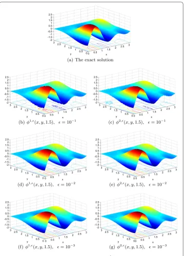
and= –. In Figure , we show the D representation of the exact solution and the
Figure 6 3D graphs ofφ(x,y) and two regularized solutionsφi,(x,y).
5 Conclusion
The study on the inverse Poisson-type problem with inhomogeneous source in D and D is still limited. This work is a continuous development of our previous study.
second method. The numerical results prove the efficiency of the theoretical suggestion, i.e., regularized solutions stably converge to the exact solution.
Competing interests
The authors declare that they have no competing interests.
Authors’ contributions
All authors contributed equally and significantly in writing this paper. All authors read and approved the final manuscript.
Author details
1Faculty of Mathematics and Statistics, Ton Duc Thang University, Ho Chi Minh City, Vietnam.2Department of
Mathematics and Applications, Sai Gon University, Ho Chi Minh City, Vietnam.3Environmental Science Lab, Institute for
Computational Science and Technology, Ho Chi Minh City, Vietnam.
Acknowledgements
This research is funded by the Foundation for Science and Technology Development of Ton Duc Thang University (FOSTECT) under project named ‘Inverse problem for inhomogeneous parabolic and elliptic equations’. The authors would like to thank the anonymous referees for their valuable suggestions and comments leading to the improvement of our manuscript.
Received: 19 February 2014 Accepted: 11 September 2014 Published: 13 October 2014
References
1. Beskos, DE: Boundary element method in dynamic analysis: part II (1986-1996). Appl. Mech. Rev.50, 149-197 (1997) 2. Chen, JT, Wong, FC: Dual formulation of multiple reciprocity method for the acoustic mode of a cavity with a thin
partition. J. Sound Vib.217, 75-95 (1998)
3. Harari, I, Barbone, PE, Slavutin, M, Shalom, R: Boundary infinite elements for the Helmholtz equation in exterior domains. Int. J. Numer. Methods Eng.41, 1105-1131 (1998)
4. Hall, WS, Mao, XQ: A boundary element investigation of irregular frequencies in electromagnetic scattering. Eng. Anal. Bound. Elem.16, 245-252 (1995)
5. Zhdanov, MS, Keller, GV: The Geoelectrical Methods in Geophysical Exploration. Methods in Geochemistry and Geophysics, vol. 31. Elsevier, Amsterdam (1994)
6. Cannon, JR: Error estimates for some unstable continuation problems. J. Soc. Ind. Appl. Math.12, 270-284 (1964) 7. Charton, M, Reinhardt, H-J: Approximation of Cauchy problems for elliptic equations using the method of lines.
WSEAS Trans. Math.4(2), 64-69 (2005)
8. Douglas, J Jr.: A numerical method for analytic continuation. In: Boundary Value Problems in Difference Equation, pp. 179-189. University of Wisconsin Press, Madison (1960)
9. Elden, L, Berntsson, F: A stability estimate for a Cauchy problem for an elliptic partial differential equation. Inverse Probl.21, 1643-1653 (2005)
10. Hao, DN, Hien, PM: Stability results for the Cauchy problem for the Laplace’s equation in a strip. Inverse Probl.19, 833-844 (2003)
11. Kubo, M:L2-Conditional stability estimate for the Cauchy problem for the Laplace’s equation. J. Inverse Ill-Posed
Probl.2, 253-261 (1994)
12. Qian, Z, Fu, CL, Xiong, XT: Fourth-order modified method for the Cauchy problem for the Laplace’s equation. J. Comput. Appl. Math.192, 205-218 (2006)
13. Qian, Z, Fu, CL, Ping, Z: Two regularization methods for a Cauchy problem for the Laplace’s equation. J. Math. Anal. Appl.338(1), 479-489 (2008)
14. Cannon, JR, Miller, K: Some problems in numerical analytic continuation. J. Soc. Ind. Appl. Math., Ser. B Numer. Anal.2, 87-98 (1965)
15. Regi ´nska, T, Tautenhahn, U: Conditional stability estimates and regularization with applications to Cauchy problems for the Helmholtz equation. Numer. Funct. Anal. Optim.30, 1065-1097 (2009)
16. Regi ´nska, T, Wakulicz, A: Wavelet moment method for the Cauchy problem for the Helmholtz equation. J. Comput. Appl. Math.223(1), 218-229 (2009)
17. Lesnic, D, Elliott, L, Ingham, DB: The boundary element solution of the Laplace and biharmonic equations subjected to noisy boundary data. Int. J. Numer. Methods Eng.43, 479-492 (1998)
18. Tautenhahn, U: Optimal stable solution of Cauchy problems for elliptic equations. Z. Anal. Anwend.15, 961-984 (1996)
19. Wei, T, Chen, YG: A regularization method for a Cauchy problem of Laplace’s equation in an annular domain. Math. Comput. Simul.82(11), 2129-2144 (2012)
20. Zhang, H, Wei, T: An improved non-local boundary value problem method for a Cauchy problem of the Laplace equation. Numer. Algorithms59(2), 249-269 (2012)
21. Wei, T, Zhou, DY: Convergence analysis for the Cauchy problem of Laplace’s equation by a regularized method of fundamental solutions. Adv. Comput. Math.33(4), 491-510 (2010)
22. Showalter, RE: Regularization and approximation of second order evolution equations. SIAM J. Math. Anal.7(4), 461-472 (1976)
23. Qin, HH, Wei, T: Some filter regularization methods for a backward heat conduction problem. Appl. Math. Comput. 217(24), 10317-10327 (2011)
doi:10.1186/1687-1847-2014-258