R E S E A R C H
Open Access
Estimation of parameters in a structured
SIR model
Begoña Cantó
*, Carmen Coll and Elena Sánchez
*Correspondence:
[email protected] Instituto de Matemática Multidisciplinar, Universitat Politècnica de València, Camino de Vera, 14, Valencia, 46022, Spain
Abstract
In this paper, an age-structured epidemiological process is considered. The disease model is based on a SIR model with unknown parameters. We addressed two important issues to analyzing the model and its parameters. One issue is concerned with the theoretical existence of unique solution, the identifiability problem. The second issue is how to estimate the parameters in the model. We propose an iterative algorithm to study the identifiability of the system and a method to estimate the parameters which are identifiable. A least squares approach based on a finite set of observations helps us to estimate the initial values of the parameters. Finally, we test the proposed algorithms.
Keywords: epidemic process; mathematical modeling; parameter estimation; identifiability; discrete-time system
1 Introduction and problem statement
In the past decades, dynamical systems have been used to develop models in physics, bi-ology, chemistry, engineering and epidemiology; see for instance [, ] and []. Usually equations modeling these phenomena depend on several parameters. Some of them have a scientific meaning and others might come from approximations. Unfortunately, most of the parameters are unknown. Then the parameter estimation is essential for modeling biological systems. Moreover, to execute a parameter estimation task, first one needs to ensure the identifiability of the system, since if the number of unknown parameters is very large, it is often impossible to find a unique solution to this problem.
Identification of systems deals with the problem of modeling of systems in which pre-vious information available is not sufficient to determine all the parameters involved in the model. The identification property has been studied on topics related with dynamic systems [–]. Parameter estimation is the process of trying to calculate the model param-eters based on a dataset. Often, some of the paramparam-eters can be measured, while the rest can only be fitted. A crucial tool in the fitting process is assigning of the parameter values so that the errors between the measured variables and the corresponding model predic-tions are minimized. The process consists in assuming that the values of the parameters of a given system are unknown, but that we have recorded inputs and outputs over a time interval. The usual estimation methods include the projection algorithm, gradient algo-rithm, and least squares algorithm [, ].
Therefore, real data are needed to construct and validate models. The identification and estimation problems will be used to find the model that best fits the data from a set of candidates. Finally, it is necessary to evaluate and to validate if the model satisfies the process properties.
In this paper, parameter estimation for an epidemic model has been tackled in the frame-work of control theory. The algorithm is developed by exploiting the special structure of our model.
Consider a nonlinear system representing an epidemiological model given by
x(k+ ) =fx(k), p, k∈Z,
wherex(k)∈Rnis the state vector, p∈Rlis the parameter vector andf:Rn×Rl→Rnis a continuously differentiable function. This system can be linearized around the disease free equilibrium point which is defined as the equilibrium point where no disease is present in the population. In our problem this linear system is of the type
x(k+ ) =A(p)x(k) +b, k∈Z, ()
where A(p)∈Rn×nandb∈Rn. The matrix coefficients have a fixed structure and it is now interesting to obtain the parameters required by the model structure. This property is known as the identifiability problem. Given a parameterized model it is important to uniquely identify the parameters since it is necessary to do experimental design and to estimate the unknown parameters of the model using experimental data.
The identifiability problem is based on the determination of all parameter sets which give the same input-output response. The identifiability of the system () depends on if the parameters can be determined uniquely from a known output of the system []. That is, given two parameter vectors p,p¯, if we denote byxp(k) and xp¯(k) the output of the system (), respectively, then the equationxp(k) =xp¯(k), for allk≥, implies p =p¯.
For linear models there are many well-established techniques to analyze structural iden-tifiability; see, for example, [–] and the references therein.
After analyzing the identifiability property we consider the estimation problem. Param-eter estimation is an important issue in biological systems because it is useful for obtain-ing predictions of computer models of biological systems step. This problem is usually addressed by fitting model simulations to the observed experimental datasetob(i)∈Rn, i= , . . . ,K. The filter is well known in control and estimation theory and has application in a wide range of fields such as epidemiology, weather forecasting and economy.
To solve the estimation problem we rewrite the system () obtaining
x(k+ ) =M(k)p +N(k), k∈Z.
Definee(i) = (ob(i) –x(i)),i= , . . . ,K eK=col(e(i))Ki=–, and
dK=col
d(i)Ki==colob(i) –N(i– )Ki=, HK=col
Then, forK observations, we want to find the parameter vector which minimizes the quadratic cost function
JK(p) =
K
i=
e(i)Te(i)
= e
T KeK
=
(dK–HKp) T(d
K–HKp).
Efficient parameter estimation methods can be found in the literature. A common prin-ciple for most of them is to minimize the error between the observed and predicted quan-tities, often reaching a local optimum, and getting the solution requires intensive com-putation. One of the most usual methods for estimating parameters is a gradient-based regression algorithm. A good overview of different methods developed to estimate the parameters can be found in [].
2 Age-structured SIR model. Identifiability
In this work we study the parameter estimation of an age-structured SIR model where the individuals are organized in compartments from an age range. The age structure is critical in modeling epidemics caused by certain common diseases such as measles and influenza or sexually transmitted diseases (STD); one that many people are worried about getting is HIV. The choice of this type of structure is because the outcome of the epi-demic may depend sensitively on the contact structure, the recovery rate, and the death rate. For example, to analyze an infectious disease such as measles, the population can be divided into five age groups or compartments, the age grouping -, -, -, -, +, corresponding to the main school grades in Spain. So, we propose a discrete age-structured SIR model on the basis of age has great influence on the spread of infec-tious disease. It is formulated using the usual parameters in mathematical epidemiology. For different values of this parameter we can get different types of infections. That is, we divide thee population intomcompartments according to their ages but these com-partments need not have the same range of ages. Thus, we have susceptible individuals Si, infected individualsIi and recovered individualsRi at theith age compartment, for i= , . . . ,m.
We consider that only the individuals of the same age range are in contact, so the susceptible individuals only are infected from the infected individuals of its compart-ment.
We take account the transference of individuals from theith compartment to the (i+ )th compartment when they change the age range in the dynamic process and, moreover, we consider the entry of new individuals inS proportional to the size of the population
β(k)N, in order for the size the populationNto remain constant.
Figure 1 Dynamic process betweenmage compartments at timek.
Table 1 Parameters in an age compartment-structured SIR model.
Parameters atith compartment
pi,qi,ri Survival rates ofSi,Ii,Ri.
αi Exposition rate of susceptible individualsSiby contact with infected individualsIi.
γi Rate of infected individuals becoming recovered individuals.
σi,μi,νi Rate individuals changing of age-compartment without changing the state.
i,δi Rate individuals changing of age-compartment with changing the state.
whereK= ( –p+σ+σ)( –p) +σσ, we obtain the following linear discrete-time
From the above equations we obtain some sufficient conditions to ensure that the system has positive solutions, that is,Si(k),Ii(k), andRi(k),i= , , , are nonnegative for all initial conditions. For this purpose, we give the next result.
Proposition Consider the parameters pi,qi,ri, αi,γi, νi, i= , , ,andσj,μj,j= , of the model.If pi≥σi+αi,qi≥γi+μi,i= , ,p≥α,q≥γand I(k)≤θN where
θ =mini=,,{piα–iσi},withσ= ,then Si(k),Ii(k),Ri(k),i= , , ,are nonnegative for all
initial conditions.
Note that these conditions on the parameters are consistent. It is logical that the rate of individuals who move from one compartment to another plus the rate of individuals who recover from the disease do not exceed the rate of survival in each compartment.
2.1 Algorithm to identifiability of the parameters
We assume that the ratesσi,μiandνi,i= , , , and the ratesiandδi,i= , , are known. Then the parameters to identify are the following:
p= (pi,qi,ri,γi,αi,i= , , ).
identifiability helps us test the unique relationship between parameter sets and model re-sponse and guarantees that the parameters can be estimated under ideal conditions. It is important to check the identifiability property since if a model is not correctly formulated, problems can appear in the parameter estimation.
Denoting the solution of the system () byxp(k) we havexp(k) =A(p)kx() + k–
i=A(p)ib. To identify the parameters we consider different initial statesx() and supposexp(k) = xp¯(k) for allk≥ from two parameters p andp¯. Then we want to prove that p =p¯.
Specif-ically, we identify all the parameters, exceptp.
In order to solve this identifiability problem in general, that is, when we havem≥ age compartments, we give the following algorithm.
Algorithm
Step Input data:m(number of compartments),N(population);σi,μiandνi,
i= , , ;iandδi,i= , .
Step Input variable parameters:pi,qi,ri,γi,fi,i= , , , andp¯i,q¯i,¯ri,γ¯i,f¯i,i= , , .
Step Obtainn= mand introduce canonical vectors{ei}ni=.
Step Constructb,A(p), andA(p¯)as in ().
Step For eachi= , . . . ,n, construct the outputxp()andxp¯()of the system ()
obtained fromx() =Nei, which we denote by{x(i, , p)}ni=and{x(i, ,p¯)}ni=,
respectively.
Step Fori= , . . . ,n:
Step . For eachl= , . . . ,n, thelth row ofx(i, , p)is denoted asx(i, , p)l.
Step . Ifx(i, , p)l≥for alll, then solvex(i, , p) =x(i, ,p¯)and save the
identified variable parameters.
Step . Else check if all parameters are identified and go to Step . Otherwise, go to Step .
Step t=i
Step . Input initial data{S
h,Ih}such thatSh+Ih=Nbeingt= (h– ) + and
construct initial conditionsx() =S
het–+Ihet, denoted byxˆ(t, ).
Step . Construct the output of the system () at timek= obtained from
ˆ
x(t, )for each parameterp, andp¯which we denote by{ˆx(t, , p)}nt=
and{ˆx(t, ,p¯)}ni=, respectively.
Step . Solvexˆ(t, , p) =xˆ(t, ,p¯)and save the identified parameters.
Step . i=t+ . Ifi=n+ , then go to Step . Otherwise, return to Step ..
Step Using the definition ofSfi andfi, the parametersαiare identified.
Step All parameters are identified, exceptp, END.
In the process specified in the algorithm we have considered the nonnegativity of the solution. For this purpose, we have had to use the solution of the system to the initial conditions constructed at Step to obtain nonnegativity outputs.
3 Parameter estimation
Now, we consider that the survival rates pi=p,qi=qandri=rare known. It assumes what ecologists refer to as Type II mortality, which is a constant mortality rate over the entire life span. This pattern is approached by most birds and some mammals []. Basi-cally, Type II mortality is a good approximation for the survival rate of human populations in the developed world. Furthermore, we suppose known the transference rates between consecutive compartmentsσi,μi, andνi,i= , , , andiandδi,i= , . Thus, from an observed dataset our goal is to find an approximate value of the parametersfi(from them we haveαi) and the parametersγi, using the mathematical model given by (). Note that
αiandγiare the most important rates since they give us information as regards the dis-ease under consideration. That is, for each age range, we want to have an estimated value of the rate of infection of a susceptible individual and the rate of recovery of an infected individual, which allow us to draw conclusions on the incidence of the disease according to the age of the individual.
From an initial observationob(), we consider an observed dataset
ob(k)Kk==S(k) S(k) S(k) I(k) I(k) I(k) R(k) R(k) R(k) TK
k=,
inKsteps,K≥, and, on the other hand, we have the fit mathematical model
x(k+ ) =A(p)x(k) +B, x() =ob(), k≥,
where, from now on, the parameter vector to estimate is
p=
f f f γ γ γ T
.
Rewriting the system () we have
andN(k) =col(Ni(k))i=where
N(k) =N–p
i=
Si(k) –q
i=
Ii(k) –r
i=
Ri(k) –σS(k),
N(k) =hI(k), N(k) = (r–ν)R(k),
N(k) =σS(k) + (p–σ)S(k), N(k) =μI(k) +hI(k),
N(k) =νR(k) + (r–ν)R(k), N(k) =σS(k) +pS(k),
N(k) =μI(k) +qI(k), N(k) =νR(k) +rR(k).
From theKdata of the observed dataset we want to estimate the value of p, that is, we want to find the parameter vector which minimizes the quadratic function
JK(p) =
(dK–HKp) T(d
K–HKp).
Thus, p satisfies
∂JK(p)
∂p =H T
KHKp–HKTdK= .
Note that ifSK=HkTHKis nonsingular, then the solution is p =S–KHKTdK, and if it is singu-lar, then p =S†KHT
KdK where†denotes the M-Penrose generalized inverse matrix. In this last case, p is not identifiable since we have infinite values for the parameter and a unique output of the mathematical model.
From the structure of the matrices we can establish the following result.
Proposition Let the system be().The estimation problem has a unique solution if and only if for each i,i= , , ,there exists ki, ≤ki≤K such that Ii(ki)= .
Proof If for eachi,i= , , there existski, ≤ki≤Ksuch thatIi(ki)= thenrank(Hk) = fork=max{ki}. Hence,rank(SK) = . Conversely, ifrank(SK) = , fromSK=HKTHKand using the structure of the matricesHK andM(k) the condition is proved. Therefore, we can ensure thatSKis definite positive, that is, all eigenvalues are positive and there exists S–
K for allK>k.
Under the above assumption, we could obtain an approximated value of p, for instance, using the descendent gradient method. That is, from an initial pthe (i+ )th step provides us
pi+= pi–ai
SKpi–HKTdK
= pi+aiHKT(dK–HKpi),
The parameter p≥ chosen in this epidemiological model satisfiesp < , where · denote the spectral norm. In the next result we establish a condition on the observed dataset in order to keep this property in the process of parameter estimation.
Proposition Let the system be().For each i,i= , , ,we suppose that there exists ki, ≤ki≤K such that Ii(ki)= .
IfdK<
ρ(S– K)
ρ(SK)
thenpK< ,
wherepK =S–KHKTdK is the parameter which minimizes the problem associated with K observation data andρ(·)denoting the spectral radius.
Proof From pK=Sk–HKTdKand taking into account thatSKis a symmetric matrix
pK=S–KHKTdK≤ρ
S–KHKdk<ρ
S–Kρ(SK)dK< .
3.1 Adding more observations. Algorithm
ConsiderKdata of the observed dataset, such thatIi(ki)= for some ki, ≤ki≤Kand for eachi,i= , , . This fact implies that there existsksuch thatH(k) is full rank. Now, we want to improve the approximated value of parameter p adding one observationob(K+ ) and fitting the mathematical model to theK+ data of the observed dataset. Using that
HKT+HK+=HKTHK+MT(K)M(K),
HKT+dK+=HKTdK+MT(K)d(K+ ),
we obtain the following discrete-time variable system to represent the dynamic of the parameter vector:
pK+=AKpK+BK, K≥, ()
whereAK=S–K+SKandBK=S–K+MT(K)d(K+ ), whereSK=HKTHK. The solution of this system is
pK=A(K,k)pk+ K–
j=k+
A(K,j+ )Bj, K>k,
with the monodromy matrixA(K,k) defined asA(K,k) =AK–· · ·AkifK>kand
A(K,k) =IifK=k.
Note that if AK is asymptotically stable, that is, ρ(AK) < for all K >k, then the monodromy matrix is also asymptotically stable, since ρ(A(K,k)) =A(K,k) ≤ K–
k=kρ(Ak) < (this is followed from the symmetry of the matrixSK forK>k). Hence, we can ensure that the recurrence sequence of the parameter vector{pK}K≥obtained as solution of () is bounded ifBKis also bounded.
Proposition Let the system be().Suppose that there exists ksuch thatrank(H(k))
is full rank, and ρ(AK) < for all K >k. Consider the observation data such that ob(K+ ) –x(K+ )<
ρ(S–
K+)ρ(MT(K)M(K))
,for some> .Then
pK+– pK<.
Proof GivenKobservation data andAK=SK–+SK,BK=S–K+MT(K)d(K+ ) we have
pK+– pK =AKpK+BK– pK
≤S–K+(SK–SK+)pK+MT(K)d(K+ ) ≤ρS–K+MT(K)d(K+ ) –M(K)pK
=ρS–K+ρMT(K)M(K)ob(K+ ) –x(K+ )<. Remark The parameters involved in an epidemiological process are not always known. To obtain a value of these sufficiently reliable, it is necessary to know if it can be identified from a set of observations of the process, and then estimate its value. In the literature, there exist several approaches to the identifiability problem and to the estimation problem. From a set of observations, for instance in engineering, it is usual to consider the transfer matrix, in chemicals, if we consider the input-output response and the parameters of Markov [, ], or directly from the solution of the system. Generally the estimation approach is based in the gradient algorithm and the least squares algorithm, [, ]. In our case, we identify the case using the structure of the matrices and asking whether the performance of the estimation process is constructive, using a least squares algorithm. Then the algorithm proposed can be used to identify and estimate the parameters of other time-discrete age-structured models taking into account only the structure one has when performing the steps of our algorithm.
4 Numerical example
Consider an age-structured population in three compartments which may suffer a con-tagious disease. We consider that the survival rate of susceptible, infected, and recovered individuals are independent from the age. Concretely, we havep= .,q= .,r= .. Let us consider that the rates of individuals changing compartment due to increasing age are known. Specifically, we considerσi=μi= . and=νi=δi= ., for alli.
In this process we want to obtain an estimation of the exposition and the recovered rates which we suppose different according to the age of the individual.
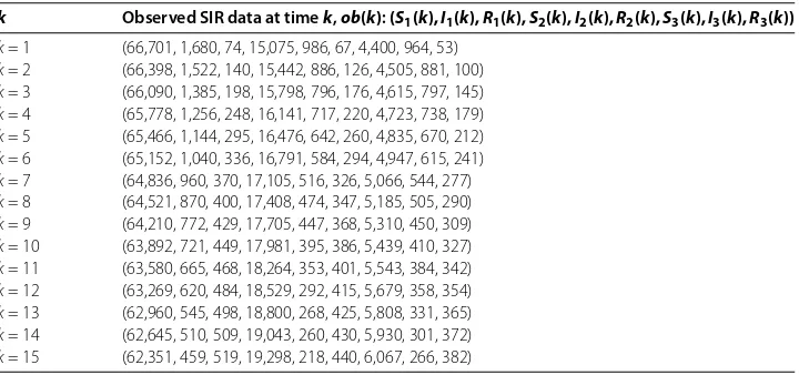
We make an experiment on a sample of size N = , from the initial condi-tion ob() = (,, ,, , ,, ,, , ,, ,, ) and an observed dataset {ob(k),k= , . . . , }, given in Table .
We see that the matrixHis full rank and the coefficient matrixAkof the discrete-time linear system given by () is stable,ρ(Ak) < , for allk= , . . . , . Applying this recurrence equation we obtain the approximations of the parameter vector p given in Table .
Note that these approximations satisfy pk≈. and pk+– pk < –, for all k= , . . . , . In fact, at timek, the condition established in Proposition holds when we compare the observed dataob(k) and the outputx(k) of the system () obtained from pk:
ob(k) –x(k)< –
Table 2 Observed dataset of SIR individuals in a population.
k Observed SIR data at timek,ob(k):(S1(k), I1(k), R1(k), S2(k), I2(k), R2(k), S3(k), I3(k), R3(k))
k= 1 (66,701, 1,680, 74, 15,075, 986, 67, 4,400, 964, 53) k= 2 (66,398, 1,522, 140, 15,442, 886, 126, 4,505, 881, 100) k= 3 (66,090, 1,385, 198, 15,798, 796, 176, 4,615, 797, 145) k= 4 (65,778, 1,256, 248, 16,141, 717, 220, 4,723, 738, 179) k= 5 (65,466, 1,144, 295, 16,476, 642, 260, 4,835, 670, 212) k= 6 (65,152, 1,040, 336, 16,791, 584, 294, 4,947, 615, 241) k= 7 (64,836, 960, 370, 17,105, 516, 326, 5,066, 544, 277) k= 8 (64,521, 870, 400, 17,408, 474, 347, 5,185, 505, 290) k= 9 (64,210, 772, 429, 17,705, 447, 368, 5,310, 450, 309) k= 10 (63,892, 721, 449, 17,981, 395, 386, 5,439, 410, 327) k= 11 (63,580, 665, 468, 18,264, 353, 401, 5,543, 384, 342) k= 12 (63,269, 620, 484, 18,529, 292, 415, 5,679, 358, 354) k= 13 (62,960, 545, 498, 18,800, 268, 425, 5,808, 331, 365) k= 14 (62,645, 510, 509, 19,043, 260, 430, 5,930, 301, 372) k= 15 (62,351, 459, 519, 19,298, 218, 440, 6,067, 266, 382)
Table 3 Estimated values of the parameter p.
Estimated value piof p from dataset{ob(k)}ik=1
p1= (0.00956693, 0.000751478, 0.00521651, 0.0407453, 0.0610622, 0.0490052)
p2= (0.00907106, 0.000369321, 0.00390195, 0.0410328, 0.0604876, 0.049093)
p3= (0.00933411, 0.000142124, 0.00248374, 0.0407704, 0.0600328, 0.0503554)
p4= (0.00927112, 0.000579406, 0.00335454, 0.0407454, 0.0599345, 0.0491128)
p5= (0.00938896, 0.000491274, 0.00304479, 0.040709, 0.060185, 0.0493809)
p6= (0.00941313, 0.00179466, 0.00343295, 0.0407295, 0.0603492, 0.0493287)
p7= (0.00981096, 0.0015837, 0.00287703, 0.0403433, 0.0609501, 0.0508397)
p8= (0.00970246, 0.00194832, 0.00285248, 0.0403566, 0.0604301, 0.0498377)
p9= (0.00927398, 0.00247651, 0.00222736, 0.0407216, 0.0597542, 0.0499973)
p10= (0.00967561, 0.00282768, 0.00192291, 0.0404139, 0.0601675, 0.0499162)
p11= (0.0100975, 0.00258414, 0.00326115, 0.0415127, 0.0617572, 0.0517111)
p12= (0.0105733, 0.00229971, 0.00304286, 0.0423655, 0.0637888, 0.0525927)
p13= (0.0105774, 0.00208498, 0.00314224, 0.0435171, 0.0644926, 0.0535962)
p14= (0.0110997, 0.00268321, 0.00341103, 0.0441655, 0.0650516, 0.0546224)
p15= (0.0110427, 0.00218739, 0.00309953, 0.0447639, 0.0659736, 0.0555352)
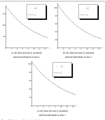
Then a good estimation of the vector can be p = (., ., ., ., ., .), such as we can see in the Figure , where the infected individuals of each age class are compared with the signal obtained when the above value of p is considered.
Note that from the definition of p = (fffγγγ)Tandf,f,fwe see that the esti-mated value to the exposition rate areα= .,α= .,α= ., and the recovery rates areγ= .,γ= .,γ= ..
5 Conclusions
(a)obI
observed andxIestimated (b)obIobserved andxIestimated
infected individuals at class infected individuals at class
(c)obI
observed andxIestimated
infected individuals at class
Figure 2 Evolution of infected individuals at each age compartment.
we have established a condition to ensure that the consecutive approximations of the pa-rameter are sufficiently close. Finally, an illustrative example has been showed.
Competing interests
The authors declare that they have no competing interests.
Authors’ contributions
The work is a product of the intellectual environment of the whole team and each author has participated equally in the work.
Acknowledgements
The authors would like to thank the referees and the editor for their comments and useful suggestions for improvement of the manuscript. This work has been partially supported by Spanish Grant MTM2013-43678-P.
Received: 21 December 2015 Accepted: 6 January 2017 References
1. Strogatz, S, Friedman, M, Mallinck-Rodt, AJ, McKay, S: Nonlinear Dynamics and Chaos: With Applications to Physics, Biology, Chemistry, and Engineering. Perseus Books, Washington (1994)
3. Han, Q, Wang, Z: On extinction of infectious diseases for multi-group SIRS models with satured incidence rate. Adv. Differ. Equ.2015, 333 (2015)
4. Cantó, B, Coll, C, Sánchez, E: Structural identifiability of a model of dialysis. Math. Comput. Model.50, 733-737 (2009) 5. Cantó, B, Coll, C, Sánchez, E: Identifiability of a class of discretized linear partial differential algebraic equations. Math.
Probl. Eng., 1-12 (2011)
6. Craciun, G, Pantea, C: Identifiability of chemical reaction networks. J. Math. Chem.44, 244-259 (2008) 7. Malik, MB, Salman, M: State-space least mean square. Digit. Signal Process.18, 334-345 (2008)
8. Ding, F, Liu, PX, Liu, G: Multiinnovatiovation least-squares identification for system modeling. IEEE Trans. Syst. Man Cybern., Part B, Cybern.18(3), 767-778 (2010)
9. Ben-Zvi, A, McLellan, PJ, McAuley, KB: Identifiability of linear time-invariant differential-algebraic systems, I. The generalized Markov parameter approach. Ind. Eng. Chem. Res.42, 6607-6618 (2003)
10. Boyadjiev, C, Dimitrova, E: An iterative method for model parameter identification. Comput. Chem. Eng.29, 941-948 (2005)
11. Ben-Zvi, A, McLellan, PJ, McAuley, KB: Identifiability of linear time-invariant differential-algebraic systems, 2. The differential-algebraic approach. Ind. Eng. Chem. Res.43, 1251-1259 (2004)
12. Dion, JM, Commault, C, van der Woude, J: Generic properties and control of linear structured systems: a survey. Automatica39, 1125-1144 (2003)
13. Chou, IC, Voit, EO: Recent developments in parameter estimation and structure identification of biochemical and genomic systems. Math. Biosci.219, 57-83 (2009)