Stability analysis for a time delayed nonlinear predator–prey model

(1)

R E S E A R C H

Open Access

Stability analysis for a time-delayed

nonlinear predator–prey model

Baiyu Xie

1

_{and Fei Xu}

2*

*_{Correspondence:}

fxu.feixu@gmail.com

2_{Department of Mathematics,}

Wilfrid Laurier University, Waterloo, Canada

Full list of author information is available at the end of the article

Abstract

In this paper, we investigate the dynamics of a time-delayed prey–predator system with

θ

-logistic growth. Our investigation indicates that the models based on delayed diﬀerential equations (DDEs) with and without delay-dependent coeﬃcient both undergo Hopf bifurcation at their corresponding positive equilibria. It is shown that stability switching occurs for the interior equilibrium of the model with

delay-dependent coeﬃcient. For the DDEs model without delay-dependent coeﬃcient, increased time delay may destabilize a stable interior equilibrium.

Keywords: Hopf bifurcation; Time-delay;

θ

-logistic growth; Prey refuge

1 Introduction

In biomathematics, the interaction and interplay between different species have been modeled by systems of differential equations. Such systems characterize the dynamics of a variety of ecosystems. By constructing an ecological model, the relationship between different species in the system is revealed. Analyzing such models yields the dynamics of the system and may give a precise prediction on the evolution of populations in the system. Recently, prey refuge has been integrated into ecological models to consider the effects of the refuges on the coexistence of different species and on the stability of equilib-ria of ecosystems [1–6]. Empirical and theoretical studies have both been carried out to illustrate the influences of prey refuge on the population dynamics of the systems. Inves-tigations indicate that the existence of prey refuge may stabilize the system and by using such refuge, the prey population may refrain from extinction [7–13].

Tsoularis and Wallace [14] performed a thorough study on a variety of growth equations to model population dynamics and presented a generalized form of the logistic growth equation. Wonlyul and Kimun [15] analyzed a general Gause-type predator–prey model and investigated the existence and non-existence of non-constant positive steady-state solutions. Motivated by the works of Tsoularis and Wallace [14], and Wonlyul and Kimun [15], we construct the followingθ-logistic growth predator–prey system with prey refuge:

˙

x=rx

1 –

x K

θ – βε

2_x2_y

1 +ε2_x2–h1x,

˙

y= βε

2_x2_y

1 +ε2_x2 –ay–h2y.

(1.1)

(2)

In system (1.1), the predator’s ﬁtness increases with the consumption of prey. If we assume that for the predator species there is a time lag between the consumption of prey and the increase of predators’ ﬁtness, then time delay should be integrated into the model. The ecological model incorporating such time delay is given by

˙

x=rx

1 –

x K

θ – βε

2_x2_y

1 +ε2_x2–h1x,

˙

y=e

–mτ_βε2_x₍_t_–_τ₎2_y₍_t_–_τ₎

1 +ε2_x₍_t_–_τ₎2 –ay–h2y,

(1.2)

wherexandyrespectively denote the densities of prey and predator, andr,K,θ,β,ε,a, andmtake positive values. In system (1.2), the prey species hasθ-logistic growth with logistic indexθ and intrinsic growth rater. Here,Kis the carrying capacity,βis the pre-dation rate of predator, and ε∈(0, 1) is the refuge rate to prey. Obviously, 1 –εis the proportion of prey that is available for the predator. We useh1andh2to denote the rate

of harvesting or the environment feedback for prey and predator, respectively. We assume that the predator has death ratea. The time lag between the consumption of prey and re-ceiving corresponding increase in predator population is denoted byτ. We thus introduce a delay-dependent coefficiente–mτ _{to describe the probability of the predators that} con-sume prey at timet–τ and still remain alive at timet. Such delay-dependent coefficient may have considerable influences on the dynamical behaviors of the model and it has not been investigated extensively in the literature. In the following, we compare the dynamical behaviors of the model with and without the delay-dependent coefficient.

System (1.2) has the initial conditions

x(η) =φ(η)≥0, y(η) =ψ(η)≥0, η∈[–τ, 0],

φ(0) > 0, ψ(0) > 0,

(1.3)

where (φ(η),ψ(η))∈C([–τ, 0],R2₊₀) is the Banach space of continuous functions mapping the interval [–τ, 0] intoR2

+0, whereR2+0={(x,y) :x≥0,y≥0}.

It follows from the fundamental theory of functional diﬀerential equations [16] that sys-tem (1.2) has a unique solutionx(t),y(t) satisfying initial conditions (1.3).

This manuscript is organized as follows. In Sect. 2, we prove that solutions to system (1.2) with initial conditions (1.3) are positive and ultimately bounded. In Sect. 3, we in-vestigate the stability of the boundary equilibria of system (1.2). In Sect. 4, we show that system (1.1) and (1.2) exhibits Hopf bifurcations at the interior equilibrium. Finally, we perform numerical analysis to illustrate the main results of this article in Sect. 5.

2 Positivity and boundedness

For model (1.2) with initial conditions (1.3), we are particularly interested in the positivity and boundedness of its solution. In this section, we prove that the solutions are positive and ultimately bounded.

2.1 Positivity of solutions

(3)

Proof Assume that (x(t),y(t)) is a solution to system (1.2) satisfying initial conditions (1.3). It follows from the ﬁrst equation of model (1.2) that

x(t) =x(0)e t

0{r[1–(x(Kζ))θ]–

βε2x(ζ)y(ζ) 1+ε2x(ζ)2 }dζ_,

implying thatx(t) is positive.

Next we show thaty(t) is positive on [0, +∞). Assume that there existst1such thaty(t1) =

0, andy(t) > 0 fort∈[0,t1). It thus follows that˙y(t1)≤0. Using the second equation of (1.2),

we obtain

˙

y(t1) =

e–mτ_βε2_x₍_t_–_τ₎2_y₍_t 1–τ)

1 +ε2_x₍_t 1–τ)2

–ay(t1) –h2y(t1)

=e

–mτ_βε2_x₍_t_–_τ₎2_y₍_t 1–τ)

1 +ε2_x₍_t 1–τ)2

> 0.

The above expression is a contradiction, which completes the proof of positivity.

In the following subsection, we show that the solutions are ultimately bounded.

2.2 Boundedness of solutions

Theorem 2.2 Positive solutions of system(1.2)with initial conditions(1.3)are ultimately bounded.

Proof Suppose that (x(t),y(t)) is a solution to system (1.2) and satisﬁes conditions (1.3). Then it follows from the ﬁrst equation of (1.2) that

˙

x≤rx

1 –

x K

θ .

Thus, we have

x(t)≤ x0K [xβ₀+ (Kβ_–_xβ

0)e–rθt]

1

θ .

That is to say,

lim sup

t→+∞ x(t)≤K.

It follows from the above discussion that, for suﬃciently smallρ, there existsT1> 0 such

that ift>T1,x(t) <K+ρ. In order to prove the boundedness of the solution, we construct

the following Lyapunov function:

(4)

Evaluating the derivative ofValong the trajectories of system (1.2) yields

for alltlarge enough. We notice thatMonly depends on the parameters of system (1.2). The above discussion implies thatx(t),y(t) is ultimately bounded.

3 Stability of the boundary equilibria

In the following, we consider the stability of the boundary equilibria of model (1.2) satis-fying initial conditions (1.3).

The characteristic equation of the model corresponding toE0= (0, 0) is

(λ–r+h1)(λ+a+h2) = 0,

whose roots are obtained as

λ1=r–h1> 0 and λ2= –a–h2< 0.

It thus follows that equilibriumE0is unstable.

The characteristic equation of the model with respect toE1= (K, 0) is obtained as

(5)

Let

one positive root. It thus follows that, for allτ ≥0, whenR0≤1, equilibriumE1is stable.

WhenR0> 1, the equilibrium is unstable.

The above results are summarized in the following conclusion.

Theorem 3.1

(i) For allτ ≥0,equilibriumE0is always unstable.

(ii) For allτ ≥0,whenR0≤1,equilibriumE1is stable,and whenR0> 1,E1is unstable.

4 The Hopf bifurcation

Hopf bifurcations have been observed in population dynamical systems [6, 17]. In this section, we investigate the Hopf bifurcation of system (1.1).

4.1 Stability of a positive equilibrium for system (1.1)

WhenR0> 1, system (1.2) admits an interior (positive) equilibriumE∗. Now, we consider

the characteristic equation of the linearized system of (1.2) near the interior (positive) equilibriumE∗. The characteristic equation is then obtained as

(6)

b3(τ) = –

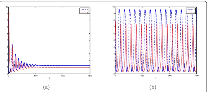
Example4.1 As an example, we choose the following system parameters (P1):r= 0.11,

K= 10,β= 0.3, a= 0.12,h1= 0.01,h2= 0.01,θ = 6, andε= 0.7. We then obtainR∗0≈

7.878654277 > 1 andA1≈0.0106755391 > 0, which guarantees that system (1.1) is stable

(see Fig. 1(a)).

In the following example, we choose (P2) as r= 0.11,K= 10,β = 0.2,a= 0.12,h1=

0.01,h2= 0.01,θ = 6, andε= 0.7. It thus follows thatR∗0≈5.055645375 > 1 and A1≈

–0.0153729314 < 0, which guarantees that system (1.1) is unstable (see Fig. 1(b)).

4.2 The Hopf bifurcation of DDEs with delay-dependent coefﬁcient

(7)

Figure 1The positive equilibriumE∗of system (1.1) is stable whenβ= 0.3 (a), and unstable whenβ= 0.2 (b). The other parameter values arer= 0.11,K= 10,a= 0.12,h1= 0.01,h2= 0.01,θ= 6, andε= 0.7. The initial condition isx0= 8 andy0= 5

Before using the criterion established by Beretta and Kuang [18] to evaluate the exis-tence of a purely imaginary root for the characteristic equation, we verify the following properties for allτ∈[0,τmax), whereτmaxis the maximum value whenE∗exists.

(a) P(0,τ) +Q(0,τ)= 0; (b) P(iω,τ) +Q(iω,τ)= 0;

(c) lim sup{|P(λ,τ)

Q(λ,τ)|:|λ| → ∞,Reλ≥0}< 1;

(d) F(ω,τ) =|P(iω,τ)|2–|Q(iω,τ)|2has a ﬁnite number of zeros;

(e) Each positive rootω(τ)ofF(ω,τ) = 0is continuous and diﬀerentiable inτwhenever it exists.

Here,P(λ,τ) andQ(λ,τ) are deﬁned by (4.2).

Assume thatτ ∈[0,τmax). It thus follows from (4.2) and (4.3) that

P(0,τ) +Q(0,τ) =b2(τ) +b4(τ) =

2β2ε4x∗3_y∗_e–mτ (1 +ε2_x∗2₎3 > 0.

Therefore,

P(iω,τ) +Q(iω,τ) = –ω2+b2(τ) +b4(τ)

+iωb1(τ) +b3(τ) = 0.

Hence, (a) and (b) are satisﬁed. It follows from (4.2) that

lim

|λ|→+∞

Q_P₍(_λλ_,,_ττ₎)= lim

|λ|→+∞

b3(τ)λ+b4(τ) λ2₊_b

1(τ)λ+b2(τ)

= 0,

which implies that condition (c) is satisﬁed. For the functionFdeﬁned in (d), it follows from

(8)

and

Q(iω,τ)2=b3(τ)2ω2+b4(τ)2

that

F(ω,τ) =ω4+a1(τ)ω2+a2(τ),

where

a1(τ) =b21(τ) – 2b2(τ) –b23(τ),

a2(τ) =b22(τ) –b24(τ).

Therefore, property (d) is satisﬁed. Assume that (ω0,τ0) is a point in its domain such that

F(ω0,τ0) = 0. It is easy to see that the partial derivativesFωandFτ exist and are

contin-uous in a certain neighborhood of (ω0,τ0), andFω(ω0,τ0)= 0. Then the implicit function

theorem implies that condition (e) is satisﬁed as well.

Next, we assume thatλ=iω(ω> 0) is a root of Eq. (4.1). Then, we substituteλ=iωinto Eq. (4.1) and separate its real and imaginary parts. Now, we obtain

ω2–b2(τ) =b3(τ)ωsinωτ+b4(τ)cosωτ,

b1(τ)ω=b4(τ)sinωτ–b3(τ)ωcosωτ.

(4.6)

From (4.6), we have

sinωτ=ω[b3(τ)(ω

2_–_b

2(τ)) +b1(τ)b4(τ)]

b3(τ)ω2+b24(τ)

, (4.7a)

cosωτ=[b4(τ) –b1(τ)b3(τ)]ω

2_–_b

2(τ)b4(τ)

b3(τ)ω2+b24(τ)

. (4.7b)

Using the deﬁnitions ofP(λ,τ) andQ(λ,τ) in (4.2), it follows from property (a) that (4.2) can be written as

sinωτ=ImP(iω,τ)

Q(iω,τ) (4.8a)

and

cosωτ= –Re P(iω,τ)

Q(iω,τ). (4.8b)

Equations (4.8a) and (4.8b) imply that

P(iω,τ)2=Q(iω,τ)2.

LetI∈R+0be the set whereω(τ) is a positive root of

(9)

Assume that, forτ∈/I,ω(τ) is not deﬁned. It thus follows that for allτ inI,ω(τ) satisﬁes

we get the following conclusion.

(10)

Construct continuous and diﬀerentiable functionsSn(τ) :I→R,

Sn(τ) =τ–

θ(τ) + 2nπ

ω(τ) , n= 0, 1, 2, . . . , (4.13)

inτ.

The following theorem is obtained using the method proposed by Beretta and Kuang [18].

It follows from Theorem 4.1 and the Hopf bifurcation theorem for functional diﬀerential equations [16] that there exists a Hopf bifurcation. Details are summarized in the following theorem.

Theorem 4.3 For system(1.2),the following conclusions hold:

(i) Assume thatR0> 1,A1> 0,and the functionS0(τ)has no positive zero inI.Then

equilibriumE∗is asymptotically stable for allτ∈[0,τmax).

(ii) Assume thatR0> 1,A1> 0,a2(τ) < 0,and the functionS0(τ)has positive zero inI.

Then there existsτ∗∈Isuch that equilibriumE∗is asymptotically stable for

τ∈[0,τ∗),and unstable forτ∈(τ∗,τmax).A Hopf bifurcation occurs whenτ=τ∗.

4.3 The Hopf bifurcation of DDEs without delay-dependent coefﬁcient

In this section, we consider the case whenm= 0, i.e., the DDEs has no terme–mτ_{. Now, all} the coeﬃcients of (4.2) are not related to the delayτ.

We denotebi=bi(0) (i= 1, . . . , 4). In this case, ifR∗0> 1 anda2(0) > 0, then Eq. (4.1) has no

positive root. Thus, the positive equilibriumE∗exists and is locally asymptotically stable for all time delayτ ≥0.

Ifm= 0,R∗₀> 1, anda2(0) < 0, then Eq. (4.1) has a unique positive rootω0, which satisﬁes

Eq. (4.9). It follows from (4.7b) that

(11)

The theorem signiﬁes that there exists at least one eigenvalue with positive real part for

τ >τ0. Diﬀerentiating Eq. (4.1) with respect toτ yields

(2λ+b1)

It follows from (4.7a)–(4.7b) that

By Rouché’s theorem [19], the root of the characteristic equation (4.1) crosses the imag-inary axis from left to right asτ is increased continuously from a number less thanτ0to

a number greater thanτ0. Therefore, both the transversality condition and the conditions

for Hopf bifurcation [16] are satisﬁed atτ=τ0. Thus, we obtain the following results for

system (1.2).

Theorem 4.4 Let m= 0,R∗₀> 1and A1> 0.For system(1.2),we have the following results: (i) Ifa2(0) > 0,then the positive equilibriumE∗of system(1.2)is asymptotically stable

(12)

(ii) Ifa2(0) < 0,then there exists a positive numberτ0such that the positive equilibrium

E∗of system(1.2)is asymptotically stable for0 <τ <τ0and is unstable forτ>τ0.We

then obtain that system(1.2)undergoes a Hopf bifurcation atE∗whenτ=τ0.

5 Numerical simulations

In this section, we use numerical simulations to verify the theoretical results obtained in previous sections.

The default parameters used in the simulations are as follows:r= 0.11,K= 10,a= 0.12, h1= 0.01,h2= 0.01,ε= 0.7, andθ = 6. Here we use numerical simulations to compare

the dynamical behaviors of the model with and without delay-dependent coeﬃcient. Four groups of simulation results with diﬀerentβandmare presented.

In simulation set (i), we choose β= 0.3 andm= 0.15 for the delay-dependent coeffi-ciente–mτ_{. For simulation set (ii), we choose the same}_β_{= 0.3 and consider the dynamical} behaviors of the model without the delay-dependent coefficient. We then compare the simulation results (i) and (ii) to reveal the effects of the delay-dependent coefficient on the system’s dynamical behaviors. In simulation set (iii), we chooseβ= 0.2 andm= 0.15 for the delay-dependent coefficiente–mτ_{. Then simulation results (iv) of the model for the} sameβ= 0.2 with the absence of the delay-dependent coefficient are presented. We

(13)

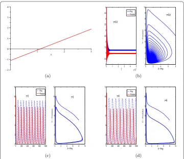
Figure 3Graph of functionS0(a). The positive equilibriumE∗of system (1.2) is stable whenτ= 0.9 (b), and unstable whenτ= 3 (c),τ= 6 (d). The other parameter values arer= 0.11,K= 10,β= 0.3,a= 0.12,h1= 0.01,

h2= 0.01,m= 0,θ= 6, andε= 0.7. Here the initial condition isx0= 8,y0= 5

pare the results (iii) and (iv) to consider the eﬀects of the delay-dependent coeﬃcient in this scenario.

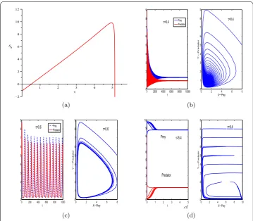
For parameter set (i), we haveτmax≈5.97 andI= [0, 5.97). The graph ofS0(τ) forτ ∈I

is shown in Fig. 2(a). As indicated in Fig. 2(a), there are two positive critical values of the delayτ, denoted byτ∗andτ∗∗, respectively. Here,τ∗≈0.5 andτ∗∗≈5.1.

(1a) Forτ= 0, as indicated in Fig. 1(a), the positive equilibrium of system (1.1) is stable. (1b) Forτ= 0.4 <τ∗, the positive equilibrium of system (1.2) is stable (see Fig. 2(b)). (1c) Forτ= 0.6∈(τ∗,τ∗∗), the positive equilibrium of system (1.2) is unstable and there

is a Hopf bifurcation whenτ=τ∗(see Fig. 2(c)).

(1d) Forτ= 5.1∈(τ∗∗,τmax), the positive equilibrium of system (1.2) is stable (see Fig. 2(d)).

For parameter set (ii), we haveτ∗≈1 (see Fig. 3(a)).

(2a) Forτ= 0, the positive equilibrium of system (1.1) is stable (see Fig. 1(a)). (2b) Forτ= 0.9 <τ∗, the positive equilibrium of system (1.2) is stable (see Fig. 3(b)). (2c) Forτ= 3.6 >τ∗, the positive equilibrium of system (1.2) is unstable

(see Fig. 3(c), (d)).

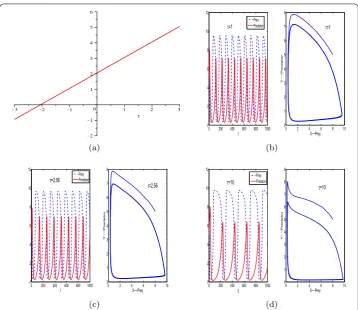
For parameter set (iii), we obtainτmax≈3.27 andI= [0, 3.27). The graph of function

S0(τ) forτ ∈Iis displayed in Fig. 4(a). As indicated in Fig. 4(a), there is only one positive

(14)

Figure 4Graph of functionS0(a). The positive equilibriumE∗of system (1.2) is unstable whenτ= 1 (b), τ= 2.65 (d), and stable whenτ= 2 (c). The other parameter values arer= 0.11,K= 10,β= 0.2,a= 0.12, h1= 0.01,h2= 0.01,m= 0.15,θ= 6, andε= 0.7. The initial condition for panels (b) and (c) isx0= 8,y0= 5. Multiple initial conditions are used for panels (d)

(3a) Forτ= 0, as indicated in Fig. 1(b), the positive equilibrium of system (1.1) is unstable.

(3b) Forτ= 1,2 <τ∗, the positive equilibrium of system (1.2) is unstable (see Fig. 4(b), (c)).

(3c) Forτ= 2.65∈(τ∗,τmax), the positive equilibrium of system (1.2) is stable and there is a Hopf bifurcation whenτ=τ∗(see Fig. 4(d)).

For parameter set (iv), as shown in Fig. 5(a), there are no positive critical values of the delayτ.

(4a) Whenτ= 0, as indicated in Fig. 1(b), the positive equilibrium of system (1.1) is unstable.

(4b) Whenτ= 1, 2.65, 10, the positive equilibrium of system (1.2) is always unstable (see Fig. 5(b), (c), (d)).

(15)

Figure 5Graph of functionS0(a). The positive equilibriumE∗of system (1.2) is always unstable whenτ= 1 (b),τ= 2.56, (c) orτ= 10 (d). The other parameter values arer= 0.11,K= 10,β= 0.2,a= 0.12,h1= 0.01,

h2= 0.01,m= 0,θ= 6, andε= 0.7. Here, the initial condition isx0= 8,y0= 5

Figure 6Bifurcation diagram of system (1.2) with the variation of delayτforr= 0.11,K= 10,β= 0.3,a= 0.12, h1= 0.01,h2= 0.01,m= 0,θ= 6, andε= 0.7

6 Conclusions

(16)

Acknowledgements

This work is supported by NSFC (No. 11326200, No. 31470641), Foundation of He’nan Educational Committee (No. 15A110015), and the Grant of China Scholarship Council (No. 201408410018).

Competing interests

The authors declare that they have no competing interests.

Authors’ contributions

All authors read and approved the ﬁnal manuscript.

Author details

1_{Department of Automation Engineering, Yellow River Conservancy Technical Institute, Kaifeng, P.R. China.}2_Department

of Mathematics, Wilfrid Laurier University, Waterloo, Canada.

Publisher’s Note

Springer Nature remains neutral with regard to jurisdictional claims in published maps and institutional aﬃliations.

Received: 3 December 2017 Accepted: 16 March 2018

References

1. Holling, C.S.: Some characteristics of simple types of predation and parasitism. Can. Entomol.91, 385–398 (1959) 2. Hassell, M.P., May, R.M.: Stability in insect host–parasite models. J. Anim. Ecol.42, 693–726 (1973)

3. Smith, J.M.: Models in Ecology. Cambridge University Press, Cambridge (1974)

4. Hassell, M.P.: The Dynamics of Arthropod Predator–Prey Systems. Princeton University Press, Princeton (1978) 5. Ji, L.L., Wu, C.Q.: Qualitative analysis of a predator–prey model with constant-rate prey harvesting incorporating a

constant prey refuge. Nonlinear Anal., Real World Appl.11, 2285–2295 (2010)

6. Wang, S.L., Ge, Z.H.: The Hopf bifurcation for a predator–prey system withθ-logistic growth and prey refuge. Abstr. Appl. Anal.2013, Article ID 168340 (2013)

7. Sih, A.: Prey refuges and predator–prey stability. Theor. Popul. Biol.31, 1–12 (1987) 8. Taylor, R.J.: Predation. Chapman & Hall, New York (1984)

9. González-Olivares, E., Ramos-Jiliberto, R.: Dynamic consequences of prey refuges in a simple model system: more prey, fewer predators and enhanced stability. Ecol. Model.166, 135–146 (2003)

10. Krivan, V.: Eﬀects of optimal antipredator behavior of prey on predator–prey dynamics: the role of refuges. Theor. Popul. Biol.53, 131–142 (1998)

11. Ma, Z.H., Li, W.L., Zhao, Y., Wang, W.T., Zhang, H., Li, Z.Z.: Eﬀects of prey refuges on a predator–prey model with a class of functional responses: the role of refuges. Math. Biosci.218(2), 73–79 (2009)

12. Chen, L.J., Chen, F.D., Chen, L.J.: Qualitative analysis of a predator–prey model with Holling type II functional response incorporating a constant prey refuge. Nonlinear Anal., Real World Appl.11, 246–252 (2010)

13. Tao, Y.D., Wang, X., Song, X.Y.: Eﬀect of prey refuge on a harvested predator–prey model with generalized functional response. Commun. Nonlinear Sci. Numer. Simul.16, 1052–1059 (2010)

14. Tsoularis, A., Wallace, J.: Analysis of logistic growth models. Math. Biosci.179, 21–55 (2002)

15. Wonlyul, K., Kimun, R.: A qualitative study on general Gause-type predator–prey models with constant diﬀusion rates. J. Math. Anal. Appl.344, 217–230 (2008)

16. Hale, J.K.: Theory of Functional Diﬀerential Equations. Springer, Heidelberg (1977)

17. Wang, S.L., Wang, S.L., Song, X.Y.: Hopf bifurcation analysis in a delayed oncolytic virus dynamics with continuous control. Nonlinear Dyn.67, 629–640 (2012)

18. Beretta, E., Kuang, Y.: Geometric stability switch criteria in delay diﬀerential systems with delay dependent parameters. SIAM J. Math. Anal.33, 1144–1165 (2002)