R E S E A R C H
Open Access
Non-polynomial cubic spline
discretization for system of non-linear
singular boundary value problems using
variable mesh
Ranjan Kumar Mohanty
1*, Sucheta Nayak
2,3and Arshad Khan
3*Correspondence: [email protected] 1Department of Mathematics, South Asian University, New Delhi, 110021, India
Full list of author information is available at the end of the article
Abstract
In this paper, we propose two generalized non-polynomial cubic spline schemes using a variable mesh to solve the system of non-linear singular two point boundary value problems. Theoretical analysis proves that the proposed methods have second-and third-order convergence. Both methods are applicable to singular boundary value problems. Numerical results are also provided to show the accuracy and efficiency of the proposed methods.
Keywords: non-polynomial; cubic spline; variable mesh; singular; non-linear
1 Introduction
In this paper, we study two effective numerical techniques using a non-polynomial cubic spline based on a variable mesh to solve system ofMnon-linear singular boundary value problems (BVPs) of the following type:
y(xxi)=F(i)x,y(), . . . ,y(i), . . . ,y(M),yx(), . . . ,y(xi), . . . ,yx(M), a≤x≤b, ()
subject to boundary conditions
y(i)(a) =Ai, y(i)(b) =Bi, wherey(xi)= dy(i)
dx ,y
(i)
xx=
dy(i)
dx ,i= , , , . . . ,M. ()
We assume that, for –∞<a≤x≤b<∞and –∞<y(i),y(i)
x <∞, wherey(i)=y(i)(x),y(xi)= y(xi)(x), we have
(i) F(i)(x,y(),y(), . . . ,y(i), . . . ,y(M),y()
x ,y()x , . . . ,yx(i), . . . ,y(xM))is continuous;
(ii) ∂∂F(i)
y(j) and
∂F(i)
∂y(xj)
exist and are continuous;
(iii) ∂∂F(i)
y(j) > and|
∂F(i)
∂y(xj)
| ≤C, for some positive constantCandi,j= , , , . . . ,M.
These conditions as proved by Keller [] ensure us of the existence of a unique solution of the above system of boundary value problem ()-().
In the present paper, we have derived generalized non-polynomial cubic spline schemes of second- and third-order using a variable mesh for solving system of two point boundary value problems ()-(). Such systems effectively decompose several higher-order problems into second-order boundary value problems; thus solving them efficiently. These higher-order problems are used to model various phenomena in the field of astrophysics, as-tronomy, hydrodynamics, beam and wave theory [–]. For these boundary value prob-lems, Aftabizadeh [], Zill [], Regan [] and Agarwal [] have obtained the existence and uniqueness of the solutions.
Many authors have developed efficient numerical schemes to solve boundary value problems and splines have been rigourously used to approximate the solution of such problems. To name a few, Mohanty et al.[–] developed AGE, cubic spline TAGE, Newton-TAGE iteration methods using a finite difference and cubic spline method based on uniform and non-uniform mesh, respectively, to solve non-linear singular two point boundary value problems. Even singularly perturbed boundary value problems with or without first derivative terms are solved. Kadalbajooet al.[] developed a third-order variable-mesh cubic spline method; Mohantyet al.used a spline in compression [, ], a spline in tension [, ], and the cubic spline TAGE method []. Wazwaz [] de-veloped modified Adomian decomposition method to solve linear and non-linear fourth-order boundary value problems, Akram and Siddiqi [] used the second-fourth-order convergent non-polynomial spline method to solve sixth-order linear special case boundary value problems. Talwar and Mohanty [] developed a finite-difference method for the solu-tion of a fourth-order ordinary differential equasolu-tion. Twizell and Boutayeb [] devel-oped finite-difference methods for solving eighth-order boundary value problems. Akram and Rehman [] solved eighth-order boundary value problems using the kernel space method. Siddiqi and Akram [, ] solved sixth- and eighth-order boundary value prob-lems using a non-polynomial and septic spline. Liu and Wu [] used a generalized dif-ferential quadrature rule to solve a special case of eighth-order boundary value problems. Also a variable mesh has been extensively used by many authors. Numerical simulations with high-order compact difference schemes depict more accurate solution values on vari-able meshes as compared to some high-order compact scheme on a uniform mesh net-work. This happens because the truncation error in a finite-difference approximation de-pends upon the derivative of the variable as well as mesh spacing. Therefore, to attain uniformly distributed truncation errors, it is essential to employ non-uniform meshes,
i.e., finer meshes in the region for largely deviated derivatives and coarse meshes for a smooth function. In this manner, the error disperses almost uniformly over the domain of integration and renders an accurate solution to a greater extent []. Such ongoing work motivated us to develop an efficient non-polynomial cubic spline scheme to solve the sys-tem of non-linear singular boundary value problems using a variable mesh.
non-linear system of coupled difference equations are solved by using the block Newton’s method.
The sections of this paper are organized as follows. In Section , we give details of deriva-tion of the scheme using a second-order singular linear boundary value problem and, in Section , we provide a generalization of the scheme. In Section , we present the appli-cation of the proposed schemes to a fourth- and sixth-order singular BVP. In Section , we discuss a convergence analysis and in Section , we provide numerical illustrations to demonstrate the accuracy of the proposed schemes. Finally in Section , we provide concluding remarks.
2 Derivation of the schemes
We consider a scalar second-order non-linear boundary value problem of the following type:
yxx=F(x,y,yx), such thaty(a) =A,y(b) =B. ()
Firstly, we discretize the solution region [a,b] such thata=x<x<x <· · ·<xN–<
xN =b. Lethj=xj–xj–,j= , , , . . . ,N, be the mesh size and the mesh ratio beσ=
hj+
hj > ,
j= , , , . . . ,N– . Whenσ = , the mesh reduces to a uniform mesh,i.e.,hj+=hj=h.
Also, assumeyjandYjto be the approximate and exact solution of () at the grid pointsxj, j= , , . . . ,N. Then the interpolating non-polynomial cubic spline approximation function can be defined as
S(x) =aj+bj(x–xj) +cjsin
k(x–xj)
+djcos
k(x–xj)
,
k> ,xj–≤x≤xj,j= , , , . . . ,N, ()
which satisfies the following conditions:
(i) S(x)coincides with a cubic polynomial in[xj–,xj],j= , , , . . . ,N. (ii) S(x)∈C[a,b].
(iii) S(xj) =y(xj),Sxxj(xj) =Fj,Sxxj(xj±) =Fj± forj= , , , . . . ,N.
Using the definition of spline () and conditions (i) and (iii) we get the following values for
aj,bj,cj,djand approximations:
aj=yj+ Fj
k, bj=
yj+–yj hj
+Fj+–Fj
kh
j
, ()
cj= – Fj
k and dj=
Fjcos(khj) –Fj+
ksin(kh
j)
, ()
Sx(xj+) = yj+–yj
hj+
+hj+(αFj+βFj+), ()
Sx(xj–) = yj–yj–
hj
–hj(γFj+βFj–), ()
Sx(xj) =
yj+β+yj(σjβ–β) –yj–σjβ
hjσj
where
α= –
θj+
– θj+ sinθj+
, γ =–
θj
– θj
sinθj
, ()
β=
θj+
–cotθj+
θj+
, β=
θj
–cotθj
θj
, ()
β=
β (σjβ+β)
, β=
β (σjβ+β)
, θj=khj and yj=y(xj). ()
Now, by the continuity conditions of first derivative,i.e., (ii), we get the following scheme:
yj+– ( +σj)yj+σjyj–=hjhj+
σjαFj++ (σjβ+β)Fj+γFj–
+Tj(hj). ()
We observe, asθj→, (α,β,β,γ)→(,,,), scheme () reduces into the standard
variable-mesh cubic spline scheme
yj+– ( +σj)yj+σjyj–=hjhj+ σ
j
Fj++ (σj+ )
Fj+ Fj–
. ()
Now, we consider the following approximations evaluated at the grid points xj, j=
, , , . . . ,N– :
sj=σj(σj+ ), ()
¯
yxj+=
( + σj)yj+– ( +σj)yj+σjyj–
hjsj
, ()
¯
yxj–=
–yj++ ( +σj)yj–σj( +σj)yj–
hjsj
, ()
¯
yxj=
yj++ (σj– )yj–σjyj–
hjsj
, ()
¯
Fj+=F(xj+,yj+,y¯xj+), ()
¯
Fj–=F(xj–,yj–,y¯xj–), ()
¯
Fj=F(xj,yj,y¯xj), ()
¯¯
yxj+=
yj+–yj hj+
+hj+(αF¯j+βF¯j+), ()
¯¯
yxj–=
yj–yj–
hj
–hj(γF¯j+βF¯j–), ()
¯¯
yxj=
yj+β+yj(σjβ–β) –yj–σjβ
hjσj
–hj+(αβF¯j+–γ βF¯j–), ()
¯¯
Fj+=F(xj+,yj+,y¯¯xj+), ()
¯¯
Fj–=F(xj–,yj–,y¯¯xj–), ()
¯¯
Simplifying ()-() and the approximations ()-(), forj= , , , . . . ,Nwe get
Now, using ()-() we generate a family of variable-mesh non-polynomial cubic spline schemes of second- and third-order for different values ofPj,RjandQjin the following
scheme:
yj+– ( +σj)yj+σjyj–=hjhj+(PjFj++QjFj+RjFj–) +Tj(hj).
(I) Second-order scheme. ForPj=σjα,Qj= (σjβ+β),Rj=γ, the local truncation errorTjisO(hj), thus leading to a second-order method.θjsatisfies the consistency
conditiontan(khj ) + (
khj ) = (
)and this equation has an infinite number of roots.
We can use the smallest positive non-zero root of the equation as the value ofθji.e., khj= ..
Note that the coefficientsPj,Qj,Rjare positive if (
√
–) <σj<
(√+)
, thus satisfying
condition of convergence of the scheme [].
3 Generalization of the schemes
β=
β (σjβ+β)
, β=
β (σjβ+β)
, θj=khj and r=j,j±, ()
Pj=
(σj+σj– )
, Qj=
(σj+ )(σj+ σj+ )
, Rj=
σj( +σj–σj)
. ()
4 Application to fourth-order singular boundary value problem We consider a linear fourth-order singular boundary value problem:
dy dx =F
x,y,dy
dx, dy dx,
dy dx
, <x≤b, ()
subject to y() =A, y(b) =B,
d
dxy() =A,
d
dxy(b) =B, ()
whereF(x,y,dxdy,ddxy,
dy
dx) =a(x)
dy
dx+b(x)
dy
dx+c(x)
dy
dx+d(x)y(x) +g(x);A,A,B,Bare real
constants and at least one of the coefficientsa(x),b(x),c(x),d(x) org(x) may be singular at
x= . We may rewrite the problem ()-() as a system of second-order boundary value problems:
dy
dx =z(x), ()
dz
dx =a(x)
dz
dx+b(x)z(x) +c(x) dy
dx+d(x)y(x) +g(x), ()
subject to
y() =A, z() =A, y(b) =B, z(b) =B. ()
Applying the difference scheme () to the coupled second-order boundary value problem ()-(), we obtain the following difference scheme:
σjyj–– ( +σj)yj+yj+=hjhj+(Pjzj++Qjzj+Rjzj–), ()
σjzj–– ( +σj)zj+zj+=hjhj+
Pj(aj+¯zxj++bj+zj++cj+y¯xj++dj+yj++gj+)
+Qj(ajz¯xj+bjzj+cjy¯xj+djyj+gj)
+Rj(aj–z¯xj–+bj–zj–+cj–¯yxj–+dj–yj–+gj–) , ()
wherePj=σjα,Qj= (σjβ+β),Rj=γ andj= , , . . . ,N– . The boundary value problem
has a singularity at somex= and hence, the scheme fails atj= . Therefore, we define the following approximations around thejth node to evade the singularity:
a∗j–=aj–hjaxj+O
hj, ()
a∗j+=aj+σjhjaxj+O
hj, ()
a∗∗j–=aj–hjaxj+ (hj)
axxj+O
hj, ()
a∗∗j+=aj+σjhjaxj+ (σjhj)
axxj+O
Similar relations forbj±,cj±,dj±,gj±can also be defined. Now, using equations ()-()
Finally, substituting ()-() in ()-(), we obtain the vector difference equation of boundary value problem ()-() as follows:
+hj
a
xj(Pj( + σj)σj+Rj) ( +σj)
+Pjσjbj
+hjσjbxjPj
,
φj = , φj= –hjσj(Pj+Qj+Rj)gj+hjσj(Pjσj–Rj)gxj . ()
Similarly, using ()-() and ()-() up toO(hj) terms in scheme () we get the second difference scheme of higher order.
4.1 Application to sixth-order singular boundary value problem
Let us consider a linear singular sixth-order boundary value problem of the following form:
dy
dx =a(x)
dy
dx +b(x)
dy
dx
+c(x)d y
dx +d(x)
dy
dx+e(x)
dy
dx +f(x)y(x) +g(x), <x≤b, ()
subject to boundary conditions:
y() =A,
d
dxy() =A,
d
dxy() =A,
y(b) =B,
d
dxy(b) =B,
d
dxy(b) =B,
()
whereA,A,A,B,B,Bare real constants and any one of the coefficientsa(x),b(x),
c(x),d(x),e(x),f(x) org(x) may be singular atx= . We may rewrite the problem ()-() as a system of second-order boundary value problems:
dy
dx =z(x), ()
dz
dx =v(x), ()
dv dx =a(x)
dv
dx+b(x)v(x) +c(x) dz
dx+d(x)z(x) +e(x) dy
dx+f(x)y(x) +g(x), ()
subject to
y() =A, z() =A, v() =A,
y(b) =B, z(b) =B, v(b) =B.
()
Applying the difference scheme () to the coupled second-order boundary value problem ()-(), we obtain the following difference scheme:
σjyj–– ( +σj)yj+yj+=hjhj+(Pjzj++Qjzj+Rjzj–), ()
σjzj–– ( +σj)zj+zj+=hjhj+(Pjvj++Qjvj+Rjvj–), ()
σjvj–– ( +σj)vj+vj+=hjhj+
Pj(aj+v¯xj++bj+vj++cj+z¯xj+
+dj+zj++ej+y¯xj++fj+yj++gj+)
+Rj(aj–v¯xj–+bj–vj–+cj–z¯xj–
+dj–zj–+ej–y¯xj–+fj–yj–+gj–), ()
wherePj,Qj,Rjare defined in Section . The boundary value problem has a singularity at x= . Therefore, as in Section we use the approximation ()-() in ()-() and we Finally, substituting ()-() in ()-(), we obtain the vector difference equation of boundary value problem () as follows:
5 Convergence analysis
We provide the vector convergence analysis for M= , i.e., a fourth-order non-linear singular boundary value problem ()-(). We apply the difference scheme () to the boundary value problem and obtain the following difference scheme:
σyj–– ( +σ)yj+yj+=hj[Pjz¯¯j++Qj¯¯zj+Rjz¯¯j–] +T(hj), ()
σzj–– ( +σ)zj+zj+=hj[PjF¯¯j++QjF¯¯j+RjF¯¯j–] +T(hj), ()
where
Pj=
(σj+σj– )
, Qj=
(σj+ )(σj+ σj+ )
, Rj=
σj( +σj–σj)
.
Now, letyˆ= (yˆ,yˆ, . . . ,yˆN–)T,zˆ= (zˆ,ˆz, . . . ,ˆzN–)T represent the exact solutions and y =
(y,y, . . . ,yN–)Tand z = (z,z, . . . ,zN–)Tbe the approximate solutions. Then we define
the error asyˆ– y = (e,,e,, . . . ,eN–,)Tandzˆ– z = (e,,e,, . . . ,eN–,)T. Next, we define
the following approximation:
ˆ¯
Fj±=F¯j±+ej±,Gj±+ (yˆ¯xj±–y¯xj±)H
j±+ej±,Vj±+ (zˆ¯xj±–¯zxj±)W
j±, ()
ˆ¯¯
Fj±=F¯¯j±+ej±,Gj±+ (yˆ¯¯xj±–y¯¯xj±)H
j±+ej±,Vj±+ (zˆ¯¯xj±–¯¯zxj±)W
j±, () ˆ¯
Fj=F¯j+ej,Gj+ (yˆ¯xj–y¯xj)H
j +ej,Vj+ (zˆ¯xj–z¯xj)W
j, ()
ˆ¯¯
Fj=F¯¯j±+ej,Gj+ (ˆ¯¯yxj–y¯¯xj)H
j +ej,Vj+ (zˆ¯¯xj–z¯¯xj)W
j, ()
where
Gr= ∂F¯
∂yr
, Hr= ∂F¯
∂yxr
, Vr=∂F¯
∂zr
, Wr= ∂F¯
∂zxr
, ()
Gr= ∂F¯¯
∂yr
, Hr=
∂F¯¯ ∂yxr
, Vr= ∂F¯¯
∂zr
, Wr= ∂F¯¯
∂zxr
, r=j,j±. ()
Further, a singularity is atx= . Therefore, we may defineGkj±,k= , , as the following approximation. Moreover, similar approximations can be also defined forHk
j±,Vjk±and
Wjk±,k= , . We have
Gkj+=Gkj +hjσGxkj +
(hjσ)
Gxx
k
j, ()
Gkj–=Gkj –hjGxkj + h
j
Gxx
k
j. ()
Thus, as we use the approximations ()-(), ()-() in equations ()-(), we get the error equation in matrix form as follows:
where E = ((e,,e,), (e,,e,), . . . , (eN–,,eN–,))T, T(hj) = ((T(h),T(h)), (T(h), T(h)), . . . , (T(hN–),T(hN–)))T, andL= (Lk,j)Nk,j–=denote the block tri-diagonal matrix. The block elements ofLare as follows:
Then, usinglj,j+lj,j–and ()-(), we get
ducible. Next we prove thatLis monotone. We let the sum of the elements of thekth row ofLbeSUMk. Then
Finally, for sufficiently smallhjand ()-(), we can easily prove thatLis monotone.
Therefore,L–exists andL–≥. Hence by () we have
E=L–T. ()
Now for sufficiently smallhjand by ()-() we can say that
SUMk≥
⎧ ⎨ ⎩
hj(P+Q+R), k= , , . . . ,N– ,
h
j(P+Q+R)(|K|+|K|), k= , , . . . ,N– ,
()
SUMk>
⎧ ⎨ ⎩
hj(R+Q), k=N– ,
h
j((R+Q)(|K|+|K|)), k=N– .
()
Sinceσ= we can say that
SUMk>max
hj(P+Q),hj(P+Q)|K|+|K|
=hj(P+Q)|K|+|K|
, fork= , , ()
SUMk≥maxhj(P+Q+R),hj(P+Q+R)|K|+|K|
=hj(P+Q+R)|K|+|K|
, fork= , , . . . ,N– , ()
SUMk>max
hj(R+Q),hj(R+Q)|K|+|K|
=hj(R+Q)|K|+|K|
, fork=N– ,N– . ()
LetL–i,kbe the (i,k)th element ofL–, then by the theory of matrices [] fori= , , . . . ,N–
L–i,k≤
SUMk
. ()
By using ()-(), we have
SUMk ≤
⎧ ⎪ ⎪ ⎪ ⎪ ⎨ ⎪ ⎪ ⎪ ⎪ ⎩
hj(P+Q)(|K|+|K|), k= , ,
hj(P+Q+R)(|K|+|K|), k= , , , . . . ,N– ,
hj(R+Q)(|K|+|K|), k=N– ,N– .
()
Now let us define
L–i,k= max ≤i≤N–
N–
k=
L–i,k and Tj= max
≤j≤N–
N–
j=
Tj(hj). ()
Therefore, as discussed in Section in scheme (),Tj(hj) =O(hj) and using (),
()-() we get
E ≤
h
j(|K|+|K|)
(P+Q)+
(P+Q+R)+
(R+Q)
Ohj=Ohj. ()
Hence, the third-order vector convergence of scheme () follows. Along similar lines, we can prove the order vector convergence of scheme () for a system of second-order boundary value problems ().
Theorem The scheme()for the numerical solution of system of non-linear singular
6 Numerical illustration
To illustrate the comparative performance of our method with existing methods, we solved the following eight problems. The root mean square errors (RMSs) in the case of a vari-able mesh, the maximum absolute error (MA) and the relative error (RE) for a uniform mesh are tabulated in Tables -. Leth=(σ(σN–)–),σ= . Therefore, the rest of thehjcan be
obtained:hj+=σhj,j= , . . . ,N– . In the case of the presence of a boundary layer near
the left or right end of the domain, take
h= ⎧ ⎨ ⎩
σ–
σN–, σ> , –σ
–σN, σ< .
This ensures the presence of mesh points in the boundary layer region near the left or right end of the interval. The linear system of difference equations have been solved by the block Gauss elimination method and the non-linear system of difference equations by the block Newton’s method in which we have consideredy= as the initial approximation. Also, without loss of generality, throughout we will use θj+=θj=θ. This does not affect the
accuracy of the scheme. All calculations have been done in Matlab .
Table 1 Example 6.1
N RMS error MA error
O(h2
j)method O(h
3
j)method O(h
4)method Ramadan [31]
8 3.6416e–03 2.5016e–05 2.0053e–06 3.010 e–05
16 1.4662e–03 5.5065e–06 1.2888e–07 1.8318 e–06
32 8.1036e–04 2.2304e–06 8.1743e–09 1.1179e–07
Table 2 Example 6.2
N RMS error MA error
O(h2
j)method O(h3j)method O(h4)method Akramet al.[21] Siddiqiet al.[32]
8 3.6473e–03 2.4393e–05 1.9706e–06 1.5379 e–06 8.1514e–05
16 1.4829e–03 5.3686e–06 1.2665e–07 1.9790 e–07 2.1052 e–05
32 8.2427e–04 2.1736e–06 8.0345e–09 4.0596 e–08 5.3084 e–06
Table 3 Example 6.3
N RMS error MA error
O(h2j)method O(h3j)method x O(h4)method Wazwaz [20]
8 2.3784e–05 1.3919e–07 0.2 5.95 e–09 1.3e–08
16 1.0736e–05 3.1300e–08 0.4 8.06 e–09 2.3e–08
32 6.2320e–06 1.2854e–08 0.6 7.26e–09 2.4e–08
64 4.2796e–06 8.0985e–09 0.8 4.34e–09 1.7e–08
Table 4 Example 6.4
N RMS error MA error
O(h2
j)method O(h
3
j)method O(h
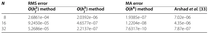
4)method Arshadet al.[33]
8 2.6861e–04 2.0392e–06 1.9385e–07 7.02e–06
16 9.2450e–05 4.6577e–07 1.2204e–08 4.35e–06
Table 5 Example 6.5
N RMS error RE error
O(h2
j)method O(h3j)method x O(h4)method Fazhanet al.[34]
40 9.6364e–02 8.3838e–03 0.40 2.9483e–05 7.5000e–04
80 6.8221e–02 5.9544e–03 0.56 2.9671e–05 7.5000e–04
160 4.8385e–02 4.2234e–03 0.72 2.9898e–05 7.2000e–04
Table 6 Example 6.6
N RMS error MA error
O(h2
j)method O(h
3
j)method O(h
4)method COC∗
8 9.9887e–05 1.3841e–05 3.0756e–05
-16 6.1365e–05 1.7426e–06 1.8795e–06 4.0324
32 4.3896e–05 5.1946e–07 1.1320e–07 4.0534
64 3.1303e–05 3.1459e–07 6.8994e–09 4.0362
Table 7 Example 6.7
N RMS error MA error
O(h2
j)method O(h
3
j)method O(h
4)method COC∗
8 3.4729e–04 1.0887e–05 2.4630e–05
-16 2.3177e–05 2.9061e–06 1.8929e–06 3.7017
32 3.8023e–05 1.4735e–06 1.3820e–07 3.7757
64 4.1196e–05 1.2815e–06 9.9099e–09 3.8018
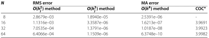
Table 8 Example 6.8
N RMS error MA error
O(h2j)method O(h3j)method O(h4)method COC∗
8 2.8679e–03 1.8940e–05 2.5391e–06
-16 1.1316e–03 3.3587e–06 1.6213e–07 3.9691
32 7.0535e–04 1.3791e–06 1.0187e–08 3.9923
64 6.4066e–04 1.1509e–06 6.3748e–10 3.9982
Example . Consider the fourth-order linear boundary value problem of the form []
dy
dx(x) –y(x) = –xcos(x) – sin(x), ≤x≤,
y() =y() = , d
dxy() = ,
d
dxy() = sin() + cos().
The exact solution is given byy(x) = (x– )sin(x). The RMS errors for a fixed value
σ = . and MA error forσ= are tabulated in Table . The graph of the exact solution versus the approximate solution using the fourth-order method forN= is given by Figure .
Example . We consider the sixth-order linear boundary value problem [, ]
d
dx+
y(x) = xcos(x) + sin(x), ≤x≤,
y() =y() = , d
dxy() = ,
d
Figure 1 Graph of the exact solution
y(x) = (x2– 1) sin(x) versus the approximate solution in fourth-order uniform mesh method forN= 32 andσ= 1 for Example 6.1.
Figure 2 Graph of the exact solution
y(x) = (x2– 1) sin(x) versus the approximate
solution in fourth-order uniform mesh method forN= 32 andσ= 1 for Example 6.2.
d
dxy() = ,
d
dxy() = –sin() – cos().
The exact solution is given byy(x) = (x– )sin(x). The RMS errors for a fixed valueσ= . and MA error forσ= are tabulated in Table . The graph of the exact solution versus the approximate solution using the fourth-order method forN= is given by Figure .
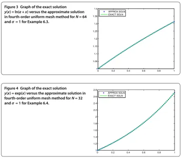
Example . Consider the fourth-order non-linear boundary value problem []:
dy
dx(x) = –exp
–y(x), ≤x≤ –e,
y() = , y( –e) =ln(), d
dxy() = –
e,
d
dxy( –e) = – .
The exact solution is given byy(x) =ln(e+x). The RMS errors for a fixed valueσ= . and MA error forσ= are tabulated in Table . The graph of the exact solution versus the approximate solution using the fourth-order method forN= is given by Figure .
Example . Consider the sixth-order non-linear boundary value problem []:
dy
dx =exp(–x)y
, ≤x≤,
y() = d
dxy() =
d
dxy() = , y() =
d
dxy() =
d
Figure 3 Graph of the exact solution
y(x) = ln(e+x) versus the approximate solution in fourth-order uniform mesh method forN= 64 andσ= 1 for Example 6.3.
Figure 4 Graph of the exact solution
y(x) = exp(x) versus the approximate solution in fourth-order uniform mesh method forN= 32 andσ= 1 for Example 6.4.
The exact solution is given byy(x) =exp(x). The RMS errors for a fixed valueσ= . and MA error forσ = are tabulated in Table . The graph of the exact solution versus the approximate solution using the fourth-order method forN= is given by Figure .
Example . Consider a sixth-order singular boundary value problem of the form []:
x( –x)d y
dx+x
dy
dx +
+exp(x)d y
dx+
+exp(x)d y
dx+xy=f(x), <x< ,
y() =y() = , d
dxy() =
d
dxy() = ,
d
dxy() =
d
dxy() = ,
where
f(x) =πxcos(πx) +– +exp(x)π+ +exp(x)π+x+ π(x– )xsin(πx).
The exact solution is given by y(x) =sin(πx). The RMS errors for a fixed valueσ = . and RE error forσ= are tabulated in Table . The graph of the exact solution versus the approximate solution using the fourth-order method forN= is given by Figure .
Example . Consider a fourth-order non-linear singular boundary value problem of the
form
d
dx+
x d
dx
y=y+cos(x)
x
Figure 5 Graph of the exact solution
y(x) = sin(πx) versus the approximate solution in fourth-order uniform mesh method forN= 160 andσ= 1 for Example 6.5.
Figure 6 Graph of the exact solution
y(x) = sin(x) versus the approximate solution in fourth-order uniform mesh method forN= 64 andσ= 1 for Example 6.6.
The exact solution is given byy(x) =sin(x). The boundary conditions are obtained from the exact solution by a test procedure. The RMS errors for a fixed valueσ= . and MA error forσ= are tabulated in Table . The graph of the exact solution versus the approximate solution using the fourth-order method forN= is given by Figure .
Example . We consider a sixth-order non-linear singular boundary value problem of
the form
d
dx+
x d
dx+
y=ey+ ex
+x
x
, <x≤.
The exact solution is given byy(x) =exp(x). The boundary conditions are obtained from the exact solution by a test procedure. The RMS errors for a fixed valueσ= . and MA error forσ= are tabulated in Table . The graph of the exact solution versus the approx-imate solution using the fourth-order method forN= is given by Figure .
Example . We consider a system of second-order boundary value problem of the form:
dy
dx=y
dz dx +z
dy
dx+f(x), ≤x≤, dz
dx=z
dz dx+y
dy dx+g(x).
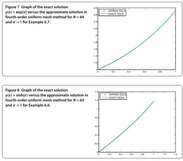
Figure 7 Graph of the exact solution
y(x) = exp(x) versus the approximate solution in fourth-order uniform mesh method forN= 64 andσ= 1 for Example 6.7.
Figure 8 Graph of the exact solution
y(x) = sinh(x) versus the approximate solution in fourth-order uniform mesh method forN= 64 andσ= 1 for Example 6.8.
σ= . and MA error forσ = are tabulated in Table . The graph of the exact solution versus the approximate solution using the fourth-order method forN= is given by Figure .
7 Conclusion
We derived second- as well as third-order variable-mesh schemes for solving linear, non-linear even-order cases and systems of second-order boundary value problems. Although, in this paper, only fourth-order and sixth-order non-linear and linear singular boundary value problems are considered, the method is general enough to implement in the case of higher even-order linear and non-linear singular boundary value problems.
present a comparative study. Hence we have compared our own results in Table , , and have also provided the computational order of convergence (COC∗) for the uniform mesh method. Our methods are also applicable to problems in cartesian as well as polar coor-dinates with minor modifications and even higher-order singularly perturbed boundary value problems can be solved easily due to the use of a variable mesh.
Acknowledgements
The authors thank the anonymous reviewers for their valuable comments, which substantially improved the paper.
Competing interests
The authors declare that they have no competing interests.
Authors’ contributions
All authors drafted the manuscript, and they read and approved the final version.
Author details
1Department of Mathematics, South Asian University, New Delhi, 110021, India.2Department of Mathematics, Lady Shri Ram College for Women, University of Delhi, New Delhi, 110024, India.3Department of Mathematics, Jamia Millia Islamia, New Delhi, 110025, India.
Publisher’s Note
Springer Nature remains neutral with regard to jurisdictional claims in published maps and institutional affiliations.
Received: 19 July 2017 Accepted: 27 September 2017 References
1. Keller, HB: Numerical Methods for Two Point Boundary Value Problems. Blaisdell Publications Co., New York (1968) 2. Bernis, F: Compactness of the support in convex and non-convex fourth order elasticity problem. Nonlinear Anal.6,
1221-1243 (1982)
3. Glatzmaier, GA: Numerical simulations of stellar convection dynamics at the base of the convection zone. Geophys. Astrophys. Fluid Dyn.31, 137-150 (1985)
4. Toomre, J, Zahn, JR, Latour, J, Spiegel, EA: Stellar convection theory II: single-mode study of the second convection zone in A-type stars. Astrophys. J.207, 545-563 (1976)
5. Terril, RM: Laminar flow in a uniformly porous channel. Aeronaut. Q.15(3), 299-310 (1964)
6. Chandrasekhar, S: Hydrodynamic and Hydromagnetic Stability. Clarendon Press, Oxford (1961). Reprinted: Dover Books, New York, 1981
7. Aftabizadeh, AR: Existence and uniqueness theorems for fourth-order boundary value problems. J. Math. Anal. Appl.
116(2), 415-426 (1986)
8. Zill, DG, Cullen, MR: Differential Equations with Boundary-Value Problems, 5th edn. Brooks/Cole, Pacific Grove (2001) 9. O’Regan, D: Solvability of some fourth (and higher) order singular boundary value problems. J. Math. Anal. Appl.
161(1), 78-116 (1991)
10. Agarwal, RP: Boundary value problems for higher order differential equations. Bull. Inst. Math. Acad. Sin.9(1), 47-61 (1981)
11. Mohanty, RK, Evans, DJ: A fourth order accurate cubic spline alternating group explicit method for non-linear singular two point boundary value problems. Int. J. Comput. Math.80, 479-492 (2003)
12. Mohanty, RK, Sachdev, PL, Jha, N: AnO(h4) accurate cubic spline TAGE method for non-linear singular two point boundary value problems. Appl. Math. Comput.158, 853-868 (2004). doi:10.1016/j.amc.2003.08.145
13. Mohanty, RK, Khosla, N: A third order accurate variable mesh TAGE iterative method for the numerical solution of two point non-linear singular boundary value problems. Int. J. Comput. Math.82, 1261-1273 (2005)
14. Kadalbajoo, MK, Bawa, RK: Third order variable-mesh cubic spline methods for singularly perturbed boundary value problems. Appl. Math. Comput.59, 117-129 (1993)
15. Mohanty, RK, Jha, N, Evans, DJ: Spline in compression method for the numerical solution of singularly perturbed two point singular boundary value problems. Int. J. Comput. Math.81, 615-627 (2004)
16. Mohanty, RK, Jha, N: A class of variable mesh spline in compression methods for singularly perturbed two point singular boundary value problems. Appl. Math. Comput.168, 704-716 (2005). doi:10.1016/j.amc.2004.09.049 17. Mohanty, RK, Evans, DJ, Arora, U: Convergent spline in tension methods for singularly perturbed two point singular
boundary value problems. Int. J. Comput. Math.82, 55-66 (2005)
18. Mohanty, RK, Arora, U: A family of non-uniform mesh tension spline methods for singularly perturbed two point singular boundary value problems with significant first derivatives. Appl. Math. Comput.172, 531-544 (2006) 19. Mohanty, RK, Evans, DJ, Khosla, N: AnO(h3) non-uniform mesh cubic spline TAGE method for non-linear singular
two-point boundary value problems. Int. J. Comput. Math.82, 1125-1139 (2005)
20. Wazwaz, A-M: The numerical solution of special fourth-order boundary value problem by the modified decomposition method. Int. J. Comput. Math.79(3), 345-356 (2002)
21. Akram, G, Siddiqi, SS: Solution of sixth order boundary value problems using non-polynomial spline technique. Appl. Math. Comput.181(1), 708-720 (2006)
23. Twizell, EH, Boutayeb, A: Finite-difference methods for the solution of special eighth-order boundary value problems. Int. J. Comput. Math.48, 63-75 (1993)
24. Akram, G, Ur Rehman, H: Numerical solution of eighth order boundary value problems in reproducing kernel space. Numer. Algorithms62, 527-540 (2013)
25. Siddiqi, SS, Akram, G: Solution of eighth-order boundary value problems using the non-polynomial spline technique. Int. J. Comput. Math.84(3), 347-368 (2007)
26. Siddiqi, SS, Akram, G: Septic spline solutions of sixth-order boundary value problems. J. Comput. Appl. Math.215, 288-301 (2008)
27. Liu, GR, Wu, TY: Differential quadrature solutions of eighth order boundary value differential equations. J. Comput. Appl. Math.145, 223-235 (2002)
28. Jha, N, Kumar, N: A fourth-order accurate quasi-variable mesh compact finite-difference scheme for two-space dimensional convection-diffusion problems. Adv. Differ. Equ.2017, Article ID 64 (2017).
doi:10.1186/s13662-017-1115-4
29. Jain, MK: Numerical Solution of Differential Equations, 3rd edn. New Age International, New Delhi (2014) 30. Varga, RS: Matrix Iterative Analysis. Prentice-Hall International, Englewood Cliffs (1962)
31. Ramadan, MA, Lashien, IF, Zahra, WK: Quintic nonpolynomial spline solutions for fourth order two-point boundary value problem. Commun. Nonlinear Sci. Numer. Simul.14, 1105-1114 (2009)
32. Siddiqi, SS, Twizell, EH: Spline solutions of linear sixth-order boundary value problems. Int. J. Comput. Math.60, 295-304 (1996)
33. Khan, A, Khandelwal, P: Solution of non-linear sixth-order two point boundary-value problems using parametric septic splines. Int. J. Nonlinear Sci.12(2), 184-195 (2011)