Dynamical analysis of a fractional SIRS model on homogenous networks

R E S E A R C H

Open Access

Dynamical analysis of a fractional SIRS model

on homogenous networks

Abstract

In this paper, we propose a fractional SIRS model with homogenous networks. The disease-free equilibrium pointE0is locally and globally asymptotically stable forR0< 1 (the disease always disappears), and endemic equilibrium pointE1is uniquely locally and globally asymptotically stable, butE0is unstable forR0> 1 (the disease is

uniformly persistent). The main results are demonstrated by numerical simulation.

Keywords: Fractional order SIRS model; Homogenous network; Local stability; Global stability; Numerical solutions

1 Introduction

Spreading of infections has been studied by researchers who used mathematical model-ing based on complex networks, which help us to understand the infections, to predict the effect of those infections on our population, to prevent and control most dangerous infec-tious diseases like HIV/AIDS, dengue fever, and H1N1 [1–3], and decide whether they are epidemic or nonepidemic. Complex networks consist of nodes and links that connect the nodes. We can represent each individual of the population, which is divided into three categories (Susceptible “x”, infected “y”, and removed “z”) as nodes, and represent links as social communication. The epidemic spreading process based on homogenous networks is discussed in [4], and we can note that the main factor in homogenous network is the average degree of nodes, which is the average contact between individuals in the popula-tion.

In [5] the modified SIRS epidemic model is introduced, and the count in a nonlinear term plays an important role in the calculation of reproductive ratioR0, which means that

the connection between individuals helps us to decide whether the disease is epidemic or free in the population. In this paper, we introduce the SIRS model supported by fractional differential equations.

It is commonly known that fractional-order systems are an extension of conventional integer-order systems. However, it should be noted that they possess advantages over the conventional integer-order systems, on which we base our work. Those advantages in-clude having memory and hereditary properties that integer-order systems do not, which are usually implemented by most biological systems. Another advantage is that fractional-order systems have a more accurate description of population models than that of the integer-order ones; they also better indicate relations between prey and predator species.

Needless to mention a wide spread of applications of fractional-order derivatives to inter-disciplinary fields. When it comes to memory and hereditary properties of materials or processes, it is often well pointed out that fractional-order calculus is best suited to their description. Such properties are all but neglected by the classical integer-order models. Considering many intriguing results found while working on models of the dynamics of population, they were found to be exclusive to integer-order differential equations [6,7].

Mainly, a great recognition and credit earned by fractional-order differential equations, as of late, has been based on the natural compatibility and better relation to systems with memory, which is found in most biological systems. Not failing to mention their relation to fractals, fractional-order systems are doubtlessly better related to them than integer-order systems, and fractals being quite abundant in biological systems, it is needless to further question the suitability of fractional-order systems to our work. Having recog-nized the need to use fractional-order systems, many biological phenomena and inter-disciplinary fields have been precisely and successfully described through models using fractional-order systems. Due to the scarcity of theories needed to analyze the dynamics of fractional-order systems, studies of stability of fractional-order population models can only be the beginning of a vast and doubtlessly fruitful implementation [6,7]. This study is also motivated by Zika epidemic [8].

In the rest of the paper, we discuss the effect of fractional differential equations and the role of networks, especially in local and global stability, and we finally support our work by numerical results. Some integral and derivative basics of the fractional order and some preliminary results are mentioned in Sect.2. In Sect.3, we give the model. In Sect.4, equilibria are calculated with studies on local stability. The global stability of equilibria is studied in Sect.5. In Sect.6, we use a numerical method (Adams-type predictor–corrector method) to solve our model in order to support the theoretical results. Finally, conclusions are summarized in Sect.7.

2 Preliminaries

First, we illustrate the definitions of the fractional-order integral, Caputo fractional deriva-tive, and Mittag-Leffler function; see [9].

Definition 2.1 The fractional integral of orderq∈R+_{of the functiong(t),t> 0, is defined}

by

Iqg(t) = t

0

(t–s)q–1

Γ(q) g(s)ds. (1)

Definition 2.2 The Caputo fractional derivative of orderq> 0 ofg(t),t> 0, is defined by

Dq_∗g(t) =In–qDng(t), (2)

whereD=d/dtandn– 1 <q≤n,n∈N.

Definition 2.3 The Mittag-Leffler function of parameterq> 0 is defined as tional dynamic model (4) if and only if

gi

yeq₁ ,yeq₂ ,yeq₃ = 0, i= 1, 2, 3.

Theorem 2.1 The equilibrium points of system(4)are locally asymptotically stable(LAS)

if all eigenvalues riof the Jacobian matrix evaluated at the equilibrium points

B=

Figure 1Stability region of the fractional-order system

Proposition 2.1([10]) The equilibrium point(yeq₁ ,yeq₂ ,yeq₃ )of system(4)is locally asymp-totically stable if one of the following conditions is satisfied:

(i) D(P) > 0,b1> 0,b3> 0,andb1b2–b3> 0.

(ii) D(P) < 0,b1≥0,b2≥0,b3> 0,andq< 2/3.

(iii) D(P) < 0,b1> 0,b2> 0,b1b2–b3= 0,and for allq∈(0, 1).

(iv) The imperative condition isb3> 0.

Now, consider the following autonomous system:

Dq_∗y(t) =g(y), q∈(0, 1). (9)

The following lemmas help us to prove the globally asymptotical stability (GAS) of equi-librium points.

Lemma 2.2(See [14]) Suppose D is a bounded closed set.Every solution of(9)starts from a point in D and remains in D all the time.If∃V(y) :D−→Rwith continuous first partial derivatives satisfies following condition:

Dq_∗V|(9)≤0.

Let E={Dq∗V|(9)= 0,y∈D},and let M be the largest invariant set of E.Then every solution

y(t)originating in D tends to M as t→ ∞.Particularly,if M={0},then y→0as t→ ∞.

Lemma 2.3(See [15]) Let y(t)∈R+_{be a continuous and differentiable function.Then,for}

any time instant t≥t0,

Dq_∗

y(t) –y∗–y∗lny(t)

y∗

≤

1 – y

∗

y(t)

Dq_∗y(t), y∗∈R+,∀q∈(0, 1). (10)

3 SIRS epidemic model on homogenous networks with fractional order (FSIRS)

Figure 2Flowchart of transmission of disease

The FSIRS model of homogenous networks is given by

Dq

∗x(t) =λ–

βkxy

x+y+z+γz– (υ+μ)x,

Dq_∗y(t) = βkxy

x+y+z– (κ+μ+α)y, (11)

Dq_∗z(t) =κy– (μ+γ)z+υx,

whereDq∗is the Caputo derivative, 0 <q≤1, and all the parametersμ,κ,λ,β,υ,γ, andα

are positive.

The parameterβrepresent the infection rate (the rate of susceptible individuals infected due to contact with infected individuals),κis the healing rate, and healed individuals be-come susceptible at the rateγ. At the same time,υrepresents the inoculation rate (suscep-tible individuals acquiring immunity by drug). The constantλis the change rate of suscep-tibles due to birth and immigration, whereμis the death rate of population independently of disease, andαis the death rate due to disease. Figure2describes the transmission of disease.

Given that the network is homogenous, we assume thatkis the average connection between nodes in the network and that all nodes have unique degrees. Also, the infection has a positive relation with population density [5].

We denote the total population asN=x+y+z.

Theorem 3.1 The closed setΩ ={(x,y,z)∈R3

+:x≥0,y≥0,z≥0,x+y+z≤ μλ}is a

positive invariant set and global attracting set of system(11).

Proof Adding three classes of system (11), we get:

Dq_∗N=λ–μN–αy,

Dq_∗N≤λ–μN.

Applying the Laplace transform, we obtain:

N(t)≤

–λ

μ+N(0)

Eq

–μtq+λ

μ,

Especially, ifN(0)≤_μλ, thenN(t)≤_μλ, since 0≤Eq(–μtq)≤1, so the closed setΩis the positive invariant set of system (11). Furthermore, sincelim_t→∞Eq(–μtq) = 0, it follows that if N(0) > _μλ, then the solutionφ(N(t)) of system (11) satisfieslimt→∞φ(N(t)) = λμ. Hence the closed setΩattracts all the solutions inR3

+, so thatΩis the global attracting

set of system (11).

4 Equilibria and their local stability

The equilibrium points of system (11) are (x0,y0,z0) = (μλ(γ(γ++μμ+)υ), 0,

The local stability ofE0andE1is studied in the following theorems.

Theorem 4.2 The disease-free equilibrium E0is locally asymptotically stable if R0< 1and

is unstable whenever R0> 1.

Proof Using the Jacobian matrix of system (11) atE0, we find that the eigenvalues are:

r1= –μ< 0,

r2= –(μ+γ+υ) < 0,

r3= –(κ+μ+α)(1 –R0) < 0.

HenceE0is locally asymptotically stable ifR0< 1.

Now, to study the local stability ofE1, we assume thatR0> 1. After evaluating the

Jaco-bian matrix of system (11) atE1, the characteristic polynomial is given by

where

So, the Routh–Hurwitz conditions are satisfied. Let D(p) denote the discriminant of polynomial (12) given by (8); using Proposition2.1, we obtain the following result.

Theorem 4.3 Assume that R0> 1.

(i) IfD(p) > 0,thenE1is locally asymptotically stable for all0 <q≤1.

(ii) IfD(p) < 0andq< 2/3,thenE1is locally asymptotically stable.

5 Global stability

The global stability ofE0andE1are studied by using a Lyapunov function.

Theorem 5.1 If R0< 1,then the disease-free equilibrium E0is globally asymptotically

sta-ble.

Proof For system (11), consider the following Lyapunov function:

L0(t) =y.

totically stable whenR0< 1, which implies that the disease will disappear regardless of the

Theorem 5.2 If R0> 1,then E1is globally asymptotically stable.

Proof Define the Lyapunov functionalL1(t) as follows:

L1(t) =x∗Φ

gleton{E1}. According to Lemma2.2and Theorem4.2,E1is globally asymptotically stable,

which implies that the disease is still at an endemic level, and it does not depend on the ini-tial density of the infected individuals. This result leads us to wonder how we can reduce the basic reproduction numberR0to be less than one.

6 Numerical methods and results

The original problem (11) is equivalent to the following fractional integral equations:

x(t) =x(0) +Iq

An Adams-type predictor–corrector method [16–18] is used for the numerical solution of fractional integral equations.

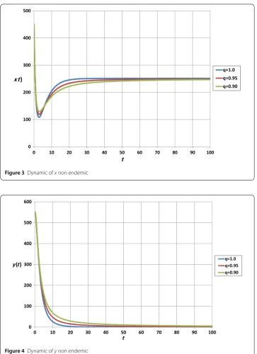
x(t),y(t), andz(t) are displayed in Figs. 3–8. In each figure, three different values of

Figure 3Dynamic ofxnon endemic

Figure 4Dynamic ofynon endemic

we setυ = 0.3, and the initial conditions are (450, 550, 0). In this case, the value ofR0

isR0= 0.602236 < 1, which means thatE0= (251.87, 0, 748.13) is globally asymptotically

stable, albeit for a large number of infected individuals at the initial time, which means the infection will die out in the population.

In Figs.6–8, we setυ= 0.005, and the initial conditions are (800, 200, 0). In this case, the value ofR0isR0= 2.27827 > 1, which means thatE0= (952.83, 0, 47.1698) is

unsta-ble, and a unique endemic equilibrium pointE1= (386.518, 87.1414, 450.528) is globally

Figure 5Dynamic ofznon endemic

Figure 6Dynamic ofxendemic

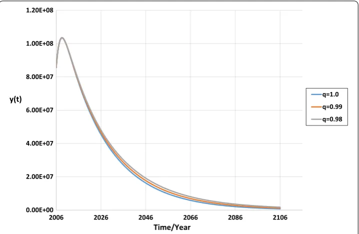
Now, we study Hepatitis B virus infection in China with clinal data [5] for the parameter values of system (11) as in Table2, with the initial conditions (4.0×108_{, 8.56×10}7_{, 6.54×}

108_).

The approximate solutionsy(t) are displayed in Figs.9–11forq= 1, 0.99, 0.98 andυ= 0.2707, 0.5, 0.9, and we find thatR0< 1.

Figure 7Dynamic ofyendemic

Figure 8Dynamic ofzendemic

Table 1 Parameter values for simulations

Parameter Value

k 6

κ 0.5

α 0.00087

γ 0.1

μ 0.001

β 0.2

λ 1

Table 2 Parameter values for simulations

Parameter Value

k 6

κ 0.073

μ 0.00714

β 0.13

α 0.0007

γ 0.01

λ 13,552,480

Figure 9Dynamic ofynon endemic (υ= 0.2707)

Consequently, we deduce that increasing the percentage (υ) of immunized population plays an important role in controlling the HBV spread. Additionally, in the fractional-order case, the peak of the infected individualsy(t) is lower, which gives more accurate results resembling real data.

7 Conclusions

In this paper, the epidemic dynamics of fractional SIRS model on homogenous networks is studied.

We show that whenR0< 1, the disease-free equilibrium pointE0is locally and globally

asymptotically stable, namely, the extinction of the disease will be achieved. WhenR0> 1,

mean-Figure 10 Dynamic ofynon endemic (υ= 0.5)

Figure 11 Dynamic ofynon endemic (υ= 0.9)

ing that the disease will persist in the population. The theoretical analysis is supported by numerical simulations. Numerical simulations show that the fractional-order case has lower peak of the infection, and the obtained results better resemble real data.

Table 3 (υ= 0.2707)

We thank Prof. E. Ahmed (Mathematics Department, Faculty of Science, Mansoura University, Mansoura, Egypt) for his support and comments.

Funding Not applicable.

Competing interests

The authors declare that they have no competing interests.

Authors’ contributions

All authors contributed equally to the writing of this paper. They read and approved the final version of the manuscript.

Author details

1_{Mathematics Department, Faculty of Science, Damietta University, New Damietta, Egypt.}2_{Mathematics & Computer}

science Department, Faculty of Science, Port Said University, Port Said, Egypt.

Publisher’s Note

Springer Nature remains neutral with regard to jurisdictional claims in published maps and institutional affiliations.

Received: 22 August 2018 Accepted: 3 April 2019

References

1. Dorogovtsev, S.N., Goltsev, A.V., Mendes, J.F.F.: Critical phenomena in complex networks. Rev. Mod. Phys.80(4), 1275–1335 (2008)

2. Xu, D., Xu, X., Yang, C., Gui, W.: Global stability of a variation epidemic spreading model on complex networks. Math. Probl. Eng.2015, Article ID 365049 (2015)

3. Newman, M.E.J.: The structure and function of complex networks. SIAM Rev.45(2), 167–256 (2003) 4. Kephart, J.O., White, S.R., Chess, D.M.: Computers and epidemiology. IEEE Spectr.30(5), 20–26 (1993) 5. Hu, Y., Mina, L., Kuang, Y.: Modeling the dynamics of epidemic spreading on homogenous and heterogeneous

networks. Appl. Anal.94(11), 2308–2330 (2014)

6. Li, H., Zhang, L., Hu, C., Jiang, Y., Teng, Z.: Dynamic analysis of a fractional order single-species model with diffusion. Nonlinear Anal., Model. Control22(3), 303–316 (2017)

7. Li, H., Ahmadjan, M., Zhang, L., Teng, Z.: Stability analysis of a fractional-order predator prey model incorporating a constant prey refuge and feedback control. Adv. Differ. Equ.2018, 325 (2018)

8. El-Saka, H.A.A., Ahmed, E.: A fractional order network model for ZIKA.https://doi.org/10.1101/039917(2016) First posted 18 Feb 2016

9. Podlubny, I.: Fractional Differential Equations. Academic Press, San Diego (1999)

10. Ahmed, E., El-Sayed, A.M.A., El-Saka, H.A.A.: On some Routh–Hurwitz conditions for fractional order differential equations and their applications in Lorenz, Rössler, Chua and Chen systems. Phys. Lett. A358, 1–4 (2006) 11. Ahmed, E., El-Sayed, A.M.A., El-Saka, H.A.A.: Equilibrium points, stability and solutions of fractional-order

predator–prey and rabies models. J. Math. Anal. Appl.325, 542–553 (2007)

13. Matignon, D.: Stability results for fractional differential equations with applications to control processing. In: Computational Eng. in Sys. Appl., Lille France, vol. 2, pp. 963–968 (1996)

14. Huo, J., Zhao, H., Zhu, L.: The effect of vaccines on backward bifurcation in a fractional order HIV model. Nonlinear Anal., Real World Appl.26, 289–305 (2015)

15. Vargas-De-León, C.: Volterra-type Lyapunov functions for fractional-order epidemic systems. Commun. Nonlinear Sci. Numer. Simul.24(1), 75–85 (2015)

16. Diethelm, K.: The Analysis of Fractional Differential Equations: An Application-Oriented Exposition Using Differential Operators of Caputo Type. Lecture Notes in Mathematics. Springer, Berlin Heidelberg (2010)

17. El-Mesiry, E.M., El-Sayed, A.M.A., El-Saka, H.A.A.: Numerical methods for multi-term fractional (arbitrary) orders differential equations. Appl. Math. Comput.160(3), 683–699 (2005)

18. El-Sayed, A.M.A., El-Mesiry, E.M., El-Saka, H.A.A.: Numerical solution for multi-term fractional (arbitrary) orders differential equations. Comput. Appl. Math.23(1), 33–54 (2004)

19. The Jakarta Post: Healthcare stumbling in RI’s hepatitis fight.