FULL PAPER
Vertical fine structure and time evolution
of plasma irregularities in the
E
s
layer observed
by a high-resolution Ca
+
lidar
Mitsumu K. Ejiri
1,2*, Takuji Nakamura
1,2, Takuo T. Tsuda
3, Takanori Nishiyama
1,2, Makoto Abo
4, Toru Takahashi
1,
Katsuhiko Tsuno
5, Takuya D. Kawahara
6, Takayo Ogawa
5and Satoshi Wada
5Abstract
The vertical fine structures and the time evolution of plasma irregularities in the sporadic E (Es) layer were observed via calcium ion (Ca+) density measurements using a resonance scattering lidar with a high time-height resolution (5 s and 15 m) at Tachikawa (35.7°N, 139.4°E) on December 24, 2014. The observation successfully provided clearer fine structures of plasma irregularities, such as quasi-sinusoidal height variation, localized clumps, “cats-eye” structures, and twist structures, in the sporadic Ca+ ( Ca+
s ) layers at around 100 km altitude. These fine structures suggested that the Kelvin–Helmholtz instabilities occurred in the neutral atmosphere whose density changed temporarily or spa-tially. The maximum Ca+ density in the Ca+
s layer was two orders of magnitude smaller than the maximum electron density estimated from the critical frequency (foEs) simultaneously observed by the ionosonde at Kokubunji (35.7°N, 139.5°E). A strong positive correlation with a coefficient of 0.91 suggests that Ca+ contributes forming the E
s layer as well as major metallic ions Fe+ and Mg+ in the lower thermosphere. Moreover, the formation of a new Ca+
s layer at 110 km and the upward motions of the Ca+
s layers at 100 km and 110 km were observed before the local sunrise and just after the sunrise time at the conjugation point. Although the presence or absence of a causal relationship with the sunrise time was not clear, a possible explanation for the formation and the upward motions of the Ca+
s layers was the occurrence of strong horizontal wind, rather than the enhancement of the eastward electric field.
Keywords: Sporadic E (Es) layer, Calcium ion (Ca+) density, Resonance scattering lidar, Mid-latitude, Vertical fine structure, Kelvin–Helmholtz instability, Ion upward flow, Lower thermosphere
© The Author(s) 2019. This article is distributed under the terms of the Creative Commons Attribution 4.0 International License (http://creat iveco mmons .org/licen ses/by/4.0/), which permits unrestricted use, distribution, and reproduction in any medium, provided you give appropriate credit to the original author(s) and the source, provide a link to the Creative Commons license, and indicate if changes were made.
Introduction
The sporadic E (Es) layer is a thin layer, typically 2–10 km
in height, with a high electron density observed between 90 and 130 km. Formation mechanisms of the Es layer
have been studied since the 1960s (e.g., MacLeod 1966; Whitehead 1961, 1970, 1989). One of the theories of the formation mechanisms for Es layer is the wind shear
theory that ions are converged in a thin layer by vertical shear of horizontal neutral wind in the lower thermo-sphere in the mid-latitude (Whitehead 1989; Mathews 1998; Haldoupis 2012). The primary ionic species for
the Es layer formation are metallic (e.g., Fe+, Mg+, Na+,
Ca+), originating from meteors. These metallic ions have a longer lifetime than the dominant species (O+, NO+, O2+) in the ionospheric E-region. Simultaneous
obser-vations of electron density and metallic Ca+ ion density in the Es layer using the incoherent scatter (IS) radar and
a resonance scattering lidar, respectively, at the Arecibo Radio Observatory (18.4°N, 66.8°W) showed that the Ca+ densities were directly related to the strength of the Es
layer (Raizada et al. 2012).
Radio and optical measurements such as radars and satellite imaging, have revealed that electron densities in the Es layers are not uniform or constant but have
irregular structures in time and space. VHF radars, including the middle and upper atmosphere (MU) radar, have observed quasi-periodic (QP) echoes, which
Open Access
*Correspondence: [email protected]
1 National Institute of Polar Research, 10-3, Midoricho, Tachikawa, Tokyo 190-8518, Japan
indicate significant perturbations in time and height in the Es layer (Yamamoto et al. 1991, 1992).
Iono-sonde observations also found the existence of irregu-lar structures by irregu-large differences between the critical (foEs) and blanketing (fbEs) frequencies, indicating the
significant variability of electron density in horizontal space (Ogawa et al. 2002). Imaging observation of Mg+ resonance scatter from a sounding rocket also observed such horizontally patchy structures in the Mg+ densi-ties, which suggest electron density irregularities in the
Es layer (Kurihara et al. 2010).
Recently, three-dimensional numerical modeling studies have suggested that plasma density irregulari-ties in the Es layer play a key role for seeding
medium-scale traveling ionospheric disturbances (MSTIDs) in the F region through ionospheric E and F region coupling process (Yokoyama and Hysell 2010; Yokoy-ama 2013). However, generation mechanisms of the plasma density irregularities in the Es layer are still
under investigation. Because the plasma density in the
E-region is about six orders smaller than the neutral density, the contribution of neutral wind dynamics to creating plasma irregular structures is significantly large. Gravity wave modulation of the Es layer is
pro-posed as one of the neutral drivers of these E-region plasma density irregularities (Woodman et al. 1991). Vertical shear of horizontal neutral wind may also drive
E-region irregularities through the plane wave pertur-bations in the altitude or density imposed on the Es
layer (Cosgrove and Tsunoda 2003, 2004; Tsunoda and Cosgrove 2004), or the Kelvin–Helmholtz (K–H) insta-bility that produces turbulence coupled to the plasma (Larsen 2000; Bernhardt 2002). The descriptions of the nonlinear evolution of these processes have been provided using numerical simulations (Cosgrove and Tsunoda 2003; Bernhardt 2002). However, spatial and temporal resolution for the Es layer was not always
suf-ficient in the IS radar and the resonance scattering lidar to determine the cause or evolution of E-region irregu-larities, though they have the capability to measure pre-cise plasma height-time variations. Thus, the observed structures could not be compared with the results of the numerical model simulations and their causes and time evolution could not be adequately explored. For example, typical height and time resolution for the Es
layer observation by the Arecibo IS radar was 300 m and 10 s, respectively (e.g., Hysell et al. 2009) and by the Ca+ resonance scattering lidar was a few hundred meters and minutes (e.g., Gerding et al. 2000; Raizada et al. 2012).
In this study, the Ca+ resonance scattering lidar devel-oped by the National Institute of Polar Research (NIPR) has measured Ca+ densities associated with the E
s layer
with a high height/time resolution of 15 m/5 s by taking advantage of the Ca+s layer, which has much higher Ca+
densities in comparison with the usual layer.
Instrumentation
Ca+ density profiles were measured using a frequency-tunable resonance scattering lidar at NIPR, Tachikawa (35.7°N, 139.4°E, 93 m height), from 11:09 to 21:26 UT on December 24, 2014. The lidar transmitter is based on an injection-seeded alexandrite ring laser for 768–788 nm (fundamental wavelengths) and a second harmonic gen-eration (SHG) unit with two harmonic crystals (Barium Borate: BBO) for 384–394 nm (second harmonic wave-lengths). The pulse width of the laser was 200–250 ns at a 25.0 Hz repetition rate, and the mean power was 0.2– 0.3 W, where the wavelength was centered at 393.477 nm. A tunable diode laser (Toptica, DL pro 780) was used as a seed laser. The laser wavelengths were tuned to the resonance frequencies utilizing a wavelength meter (HighFiness, WSU-10), which was calibrated using a wavelength-stabilized He–Ne laser. A Nasmyth-Cas-segrain f/8 telescope with 83 cm diameter primary mir-ror was used as a receiver. Photons at 393.477 nm were detected by a Hamamatsu R9880U-210 (Ultra bialkali) photomultiplier tube (PMT) attached at the back of the telescope. A band-pass filter with a center wavelength of 389.7 nm, and an FWHM of 11.5 nm was used to reduce the background sky brightness. The photon counts were recorded by a transient recorder (Licel, PR10-160-P) with a range resolution of 15 m and integrated every 125 shots (5 s). Background noise (mean photon count: 200– 230 km) was subtracted from the photon count profile, and the photon counts were normalized via the Rayleigh signal at 34–37 km to yield Ca+ densities. The minimum limit of determination was 45 cm−3.
Es layer parameters were obtained by an ionosonde
at Kokubunji (35.7°N, 139.5°E, 75 m height), located only ~ 7.5 km away from NIPR. The ionosonde is regu-larly operated by the National Institute of Information and Communications Technology (NICT). Ionograms were obtained by regular ionosonde observations every 15 min with a 15 s sweep time from 1 to 30 MHz. The field-of-view (FOV) of the ionosonde is several hun-dred km in diameter and covers the lidar FOV located at Tachikawa. Es layers were detected intermittently
throughout the night.
Observation results and discussion
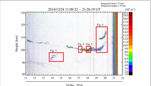
Figure 1 shows temporal variation of Ca+ density profiles observed between 11:09 and 21:26 UT on December 24, 2014. At the beginning of the observation, two sporadic Ca+ ( Ca+
s ) layers appeared at ~ 91 km and ~ 108 km.
speed of ~ 1 km/h (“main Ca+s layer” hereafter), while the
lower layer was faint. These layers became unclear from 13:45–15:00 UT, until the other layers appeared between them (~ 91–97 km). At 15:30–17:00 UT, the main Ca+s
layer appeared again and descended to ~ 100 km, while the lower layer could not be seen. After 17:00 UT, the main Ca+s layer was perturbed and showed some
insta-bility-like structures. The layer height did not change from ~ 100 km, though the layer width grew larger. At 19:15–20:15 UT, which was just before local sunrise at 100 km, the main Ca+s layer moved upward. At the same
time, another Ca+s layer appeared at 109 km and moved
upward. After 20:45 UT, background noise increased due to sunrise at ~ 100 km altitude.
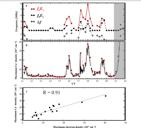
The Es layers were also observed intermittently by the
ionosonde at Kokubunji. Observed Es layer parameters,
such as the critical frequency (foEs, shown by red dots)
and blanketing frequency (fbEs, shown by black dots), are
displayed in Fig. 2a. The time after the sunrise at 100 km is demarcated by gray hatching. foEs and fbEs both
corre-spond to the maximum and minimum electron densities in the Es layer, respectively. Therefore, a large difference
(∆f) between foEs and fbEs means there is a large
differ-ence between the maximum and minimum electron den-sities within the field-of-view (FOV) of the ionosonde. During the times that the Es layer (foEs) was observed by
the ionosonde (11:00–11:30 UT, 15:30–16:15 UT, 17:00– 18:30 UT, and 19:00–19:45 UT), the Ca+ densities were relatively higher. Temporal variation of the maximum Ca+ densities at 90–120 km is shown in Fig. 2b where red dots indicate the maximum density in 10 min window, displayed every 15 min. Temporal variations of maximum Ca+ density and f
oEs in Fig. 2a, b show that the foEs was
determined from the ionogram only when the maximum Ca+ densities were larger than approximately 500 cm−3.
The correlations between the maximum Ca+ densities and the maximum electron densities estimated from foEs,
are shown in Fig. 2c. They show a strong correlation with a coefficient of 0.91 where the maximum Ca+ density was two orders of magnitude smaller than the maximum elec-tron density. These results suggest that Ca+ contributes forming the Es layer as well as major metallic ions Fe+
and Mg+ in the lower thermosphere.
Characteristic wave-like and irregular structures sur-rounded by red boxes were seen in the Ca+s layers and
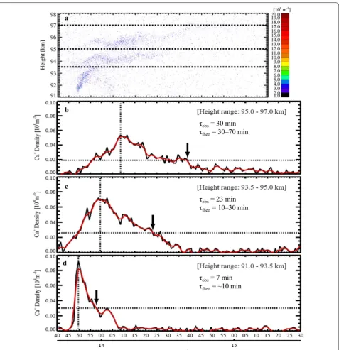
were enlarged as shown in Figs. 3, 4, 5 and 6. Figure 3a shows wave-like structures observed at 91–97 km from 13:45 UT to ~ 15:00 UT. The wave-like structures had three layers with a vertical distance of ~ 1.2 km. The upper two layers fluctuated with an observed period of ~ 15 min and moved upward with a speed of ~ 0.5 m/s. Temporal variations of average Ca+ density Fig. 3
Fig. 4 Fig. 5
Fig. 6
Fig. 1 Time-height cross section of Ca+ densities observed by the resonance scattering lidar at Tachikawa on December 24, 2014. The irregular
at 95–97 km, 93.5–95 km and 91–93.5 km are shown in Fig. 3b–d, respectively. Vertical dashed lines indicate the time when the densities were the maximum and horizontal dashed lines indicate e−1 values of the
maxi-mum densities. Ca+ density in the bottom layer became the maximum at first, followed by the middle and top layers with a time delay of ~ 9 min each. Time interval from when the density maximized to when it decreased to e−1 ( τobs ) was 7 min, 23 min, and 30 min in the
bot-tom, middle, and top layers, respectively. According to
Raizada et al. (2012), the lifetime ( τtheo ) of Ca+ in the mesosphere and lower-thermosphere region increases with height, with lifetimes in winter at 91–93.5 km, 93.5–95 km, and 95–97 km are ~ 10 min, 10–30 min, and 30–70 min, respectively. The observed time inter-vals from the peak to e−1 of densities that we identified
were comparable but slightly shorter than the theoreti-cal lifetimes. The wave-like structures may have been carried by background neutral wind. Meteoric abla-tion is a possible mechanism of the Ca+ generation
f
oE
sf
bE
s∆
f
a
b
c
UT
Maxi
mu
m
Ca
+density [1
0
2cm -3]
Maxi
mu
m
Ca
+density [1
0
2cm -3]
Maximum electron density [104cm-3]
Frequency
[MHz]
Fig. 2 Temporal variations of aEs parameters (foEs, fbEs, and ∆f = foEs−fbEs) observed by ionosonde at Kokubunji and b maximum Ca+ density at
90–120 km over Tachikawa. Red dots indicate the maximum density during ± 5 min (10 min) every 15 min. The gray hatched area indicates data obtained after local sunrise at 100 km altitude. c Is a correlation diagram of maximum Ca+ density shown by red dots in (b) and maximum electron
during the night. The Ca+ density distribution showed three layers at 91–97 km. That could be caused by three times of strong meteoric ablations from a single meteor event, which is called the “blob” structure. The Ca+ might be transported by background neutral wind into the FOV of our lidar observation, while it is diffusing
horizontally by the molecular diffusion and decreasing exponentially with the lifetime. In order to understand the mechanism of Ca+ generation, the formation of the layer structure, and the causes of the fluctuation, back-ground wind measurements with high time and height resolutions are required.
a
b
c
d
τobs= 30 min τtheo= 30–70 min
τobs= 23 min τtheo= 10–30 min
τobs= 7 min τtheo= ~10 min
Fig. 3 a Wave-like structures observed at 91–97 km from 13:45 UT to 15:00 UT. Ca+ layers, which had a distance of approximately 1.2 km, fluctuated
vertically with a period of ~ 15 min. They moved upward with a speed of ~ 0.5 m/s. Temporal variations of average Ca+ density at b 95–97 km,
The Ca+s layer at around 100–101 km (Fig. 4) showed
a vertical displacement seen as a quasi-sinusoidal vari-ation with an observed period of ~ 5 min from 17:00 to
17:11 UT. Following this variation, a localized-clump of Ca+ was formed repeatedly with an interval of ~ 2.5 min. At 17:17–17:19 UT, a “cats-eye” feature, suggesting a Fig. 4 Instability-like structures were observed at around 100 km. A “cats-eye” structure that is suggestive of large-scale deformation by neutral dynamical (Kelvin–Helmholtz) instability is clearly seen at 99.5–102 km at 17:17–17:19 UT
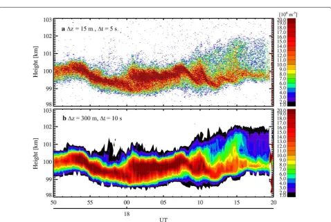
Fig. 5 Time evolution of instability structures in the Ca+
s layer at ~ 100 km is displayed with height and time integrations of 15 m and 5 s (a) and of
large-scale deformation due to K–H instability, was clearly seen at 99.5–102 km. The quasi-sinusoidal varia-tion and irregular structures are likely structures in the ionospheric ion layers that were formed in response to turbulence in the neutral atmosphere. According to a two-dimensional numerical model simulation by Bern-hardt (2002), nonlinear evolution of ion layers in the lower thermosphere in response to turbulence due to the neutral wind shear depends on a ratio of ion-neutral col-lision frequency (νi) to ion gyrofrequency (ωi). At 100 km altitude, the νi is larger than the ωi, and therefore the neu-tral wind shear generates compression and twisting of the
Es layer densities and then ultimately yields two
modu-lated layers of electron density through the K–H insta-bility structures (“cats-eye”). The localized clumps are formed where the ωi is nearly equal to the νi, such as at 120 km. The observed results with the localized clumps just before the formation of the “cats-eye” structure at ~ 100 km means the neutral density in the background was temporarily or spatially smaller than usual.
In Fig. 5a, twisted structures in the Ca+s layer,
prob-ably caused by the K–H instability, were clearly seen between 18:00 and 18:10 UT. The maximum Ca+ density in the Ca+s layer increased in time, followed by the
twist-ing of the Ca+s layer at around 18:00 UT. The twisted
structure then developed a K–H billow at around 18:10 UT. After 18:12 UT, the K–H billow disappeared, and the layer thickness became broader from 2 to 3 km. As shown in Fig. 1, this layer was then split into two mod-ulated layers with a separation of about 2 km at ~ 18:30 UT. The observed time evolution of ion layer modulation agreed with the results of numerical model simulation at ~ 100 km (Bernhardt 2002). The upper layer (~ 102 km altitude) descended after ~ 18:40 UT and merged into a single layer at ~ 18:50 UT as seen in Fig. 1. To demon-strate the capability of high time and height resolution (5 s, 15 m) by our lidar, the same Es layer observation
was plotted with a resolution of the 300 m and 10 s inte-grations, which were used as typical resolutions for the
Sunrise at 100 km at a
geomagnetic conjugate point
(19.1S,137.9E)
v
up= ~2.2 m/s
v
up= ~1.3 m/s
v
up= ~5.7 m/s
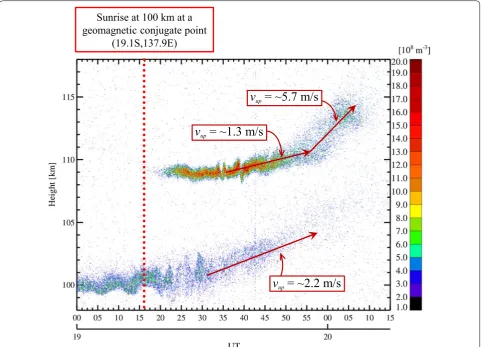
Fig. 6 Temporal variations of the Ca+
s layers observed just before sunrise (20:49 UT) at 100 km altitude over Tachikawa. The red vertical dotted line
Arecibo radar observation, in Fig. 5b. Temporal vari-ations of the maximum Ca+ density and the Ca+
s layer
thickness can be obtained, however, to reveal the detailed structures such as the twist in the Ca+s density requires
higher height-time resolution.
Figure 6 shows temporal variations of the Ca+s layers
observed just before local sunrise. The main Ca+s layer
at ~ 100 km exhibited quasi-periodic vertical oscilla-tion with a wave period of 8 min until 19:20 UT. Then, the amplitude of oscillation became larger. The layer width gradually increased between 19:00 and 19:30 from 1 to 3 km. After 19:30 UT, the oscillation was unclear but upward motion of the layer became obvious, with a speed of ~ 2.2 m/s. Together with the upward motion, the layer was faded out after 19:50 UT. Another Ca+s
layer appeared at around 19:20 UT at 109 km. This layer started to oscillate with a period of ~ 3 min at around 19:33 UT, moved upward at a rate of ~ 1.3 m/s after 19:35 UT, and then started to diffuse vertically at 19:45 UT. The upward speed increased to ~ 5.7 m/s after 19:55 UT. The sunrise time at 100 km altitude over Tachikawa was 20:49 UT, while the sunrise at the geomagnetic conjugate to Tachikawa was 19:16 UT (red dotted line in Fig. 6). In short, those, the main Ca+s layer started diffuse, a new
Ca+s layer emerged, and both layers moved upward, were
observed after the sunrise at the conjugate point but before the sunrise at Tachikawa.
In the lower thermosphere, Ca+ plays as a tracer of neutral atmospheric dynamics. However, it is well accepted that mean vertical wind is quite small (~ 0 m/s) in the mid-latitude and such upward flow is unlikely to continue more than 30 min. On the other hand, when Ca+ behaves as plasma in the E
s layer, the ion velocity ( v )
can be expressed by (Cosgrove and Tsunoda 2002)
Here B�=Bbˆ is the magnetic field, E�⊥ is the electric
field perpendicular to B , and the electric field parallel
to B has been set to zero. u is the background neutral
wind velocity. ρi is the ratio of the ion-neutral collision frequency (νi) to the ion gyrofrequency (ωi). Calculating the ion-neutral collision frequency, which was obtained from Banks and Kockarts (1973), using densities of the nitrogen and oxygen molecules and the nitrogen atoms, calculated by NRLMSISE-00 (Picone et al. 2002), ρi over Tachikawa is 34.2 at 100 km and 5.2 at 110 km.
is required. The last term has no contribution to verti-cal motion. Here, we assume that the upward motion is solely caused by the eastward electric field. The neu-tral wind is assumed to be zero. In that case, ion upward velocity ( vup ) may be written as:
where v�⊥ is the ion velocity perpendicular to B .
Accord-ing to the IGRF-12 (International Geomagnetic Refer-ence Field) model (Thebault et al. 2015), the geomagnetic inclination (I) and total magnetic field intensity (B) are derived to be 49.5° and 44,350 nT. When vup is 2.2 m/s at
100 km and 1.3 m/s and 5.7 m/s at 110 km, required EE is 176 mV/m, 2.5 mV/m, and 11 mV/m, respectively. These are quite large values in comparison with the eastward electric field (< 1 mV/m) observed at the sunrise time at Jicamarca in the equatorial region as the pre-reversal enhancement (Kelley et al. 2014). It is difficult to explain that observed upward drift of Ca+s is due to only the
�
E× �B drift driven by the eastward electric field generated
by sunrise at the conjugate point (19.1°S, 137.9°E). On the other hand, assuming that the upward motion is solely caused by the eastward neutral wind, without polariza-tion field ( E�=0 ), vup may be written as:
Again, when vup is at 100 km and 1.3 m/s and 5.7 m/s
at 110 km, it is required that uE is 116 m/s, 11 m/s, and 47 m/s, respectively. Eastward wind of 116 m/s is rela-tively fast but possible where maximum wind speed often exceeds 100 m/s in the lower thermosphere (e.g., Larsen 2002). If strong eastward wind occurs near 100 km, the new Ca+s layer could be formed above the wind
maxi-mum by a vertical shear generated by the strong east-ward wind. Therefore, an occurrence of strong easteast-ward wind around 100 km was a possible cause of the observed phenomena. In addition, the upward movement of the wind shear structure, occurring ion convergence, also could be a reason of the observed upward movement of Ca+ layer. If the wind share structure with some angles passes through the FOV of the lidar, observed height of the Ca+s layer ascends/descends with time. Although
these scenarios cannot be confirmed thoroughly without wind measurement, the observed phenomena were likely to be caused by strong horizontal winds, rather than the enhancement of the eastward electric field. However, the presence or absence of a causal relationship with the sun-rise at the conjugate point is not clear.
Summary
Vertical fine structures and the time evolution of plasma irregularities in the Es layer have been observed
via Ca+ density measurements using a resonance scat-tering lidar at Tachikawa (35.7°N, 139.4°E) on Decem-ber 24, 2014, with a high time-height resolution of 5 s and 15 m. The Ca+s layer height at around 100 km
showed quasi-sinusoidal variation at around 17:00 UT. Following this variation, the Ca+ formed local-ized clumps and the “cats-eye” structure was generated. Time evolution of twist structures was clearly observed in the Ca+s layer at around 18:00 UT. The fine
struc-tures of such plasma irregularities suggested that the K–H instabilities occurred in the neutral atmosphere whose density changed temporarily or spatially. The maximum Ca+ density in the Ca+
s layer was two orders
of magnitude smaller than the maximum electron den-sity estimated from the foEs observed by the ionosonde
at Kokubunji (35.7°N, 139.5°E), located only ~ 7.5 km away from NIPR, simultaneously. The correlation showed a strong positive correlation with a coefficient of 0.91. These results suggest that Ca+ contributes forming the Es layer as well as major metallic ions Fe+
and Mg+ in the lower thermosphere. The formation of a new Ca+s layer at 110 km altitude and the upward
motion of the Ca+s layers at 100 km and 110 km were
observed just after the sunrise time at the conjugate point and before the local sunrise. A possible explana-tion for the observed phenomena was the occurrence of strong horizontal wind, rather than the enhancement of the eastward electric field. The presence or absence of a causal relationship with the sunrise at the conjugation point and Tachikawa is still an open question.
Abbreviations
Es: sporadic E; Ca+s: sporadic Ca+; K–H: Kelvin–Helmholtz; NIPR: National
Institute of Polar Research.
Authors’ contributions
MKE (corr-auth) was involved in lidar development and observation and discussion. TN contributed to lidar development and observation and discus-sion. TT contributed to lidar development and observation. TN helped in lidar development and observation and discussion. MA was involved in lidar development. TT helped in lidar observation and discussion. KT contributed to Lidar development and observation. TDK was involved in Lidar development TO helped in Lidar development. SW contributed to Lidar development. All authors read and approved the final manuscript.
Author details
1 National Institute of Polar Research, 10-3, Midoricho, Tachikawa, Tokyo 190-8518, Japan. 2 Department of Polar Science, SOKENDAI (The Graduate University for Advanced Studies), 10-3, Midoricho, Tachikawa, Tokyo 190-8518, Japan. 3 The University of Electro-Communications, 1-5-1, Chofugaoka, Chofu, Tokyo 182-8585, Japan. 4 Tokyo Metropolitan University, 6-6, Asahigaoka, Hino, Tokyo 191-0065, Japan. 5 RIKEN, RAP, 2-1, Hirosawa, Wako, Saitama 351-0198, Japan. 6 Faculty of Engineering, Shinshu University, 4-17-1, Wakasato, Nagano 380-8553, Japan.
Acknowledgements
This work was supported by the JSPS-Kakenhi (JP15K13575), the prioritized project AJ1 and AJ0901 of Japanese Antarctic Research Expedition, and the Project Research KP2 and KP301 of the National Institute of Polar Research. The lidar data can be accessed at: http://id.nii.ac.jp/1291/00014 958/. Ionosonde data at Kokubunji were provided by the World Data Center for Ionosphere through the National Institute of Information and Communications Technol-ogy, Tokyo. The preparation of this paper was supported by an NIPR publica-tion subsidy.
Competing interests
The authors declare that they have no competing interests.
Availability of data and materials
The lidar data can be accessed at: http://id.nii.ac.jp/1291/00014 958/. Ionosonde data at Kokubunji were provided by the World Data Center for Ionosphere through the National Institute of Information and Communica-tions Technology, Tokyo.
Consent for publication
Not applicable.
Ethics approval and consent to participate
Not applicable.
Funding
The JSPS-Kakenhi (JP15K13575), the prioritized project AJ1 and AJ0901 of Japanese Antarctic Research Expedition, the Project Research KP2 and KP301 of the National Institute of Polar Research. NIPR publication subsidy
Publisher’s Note
Springer Nature remains neutral with regard to jurisdictional claims in pub-lished maps and institutional affiliations.
Received: 12 September 2018 Accepted: 2 January 2019
References
Banks PM, Kockarts G (1973) Aeronomy part A. Academic Press, New York, pp 184–239
Bernhardt PA (2002) The modulation of sporadic-E layers by Kelvin–Helmholtz billows in the neutral atmosphere. J Atmos Solar Terr Phys 54:1487–1504.
https ://doi.org/10.1016/S1364 -6826(02)00086 -X
Cosgrove RB, Tsunoda RT (2002) A direction-dependent instability of sporadic-E layers inthe nighttime midlatitude ionosphere. Geophys. Res. Lett. 29:1864. https ://doi.org/10.1029/2002G L0146 69
Cosgrove RB, Tsunoda RT (2003) Simulation of the nonlinear evolution of the sporadic-E layer instability in the nighttime midlatitude ionosphere. J Geophys Res 108:1283. https ://doi.org/10.1029/2002J A0097 28
Cosgrove RB, Tsunoda RT (2004) Instability of the E–F coupled night-time midlatitude ionosphere. J Geophys Res 109:A04305. https ://doi. org/10.1029/2003J A0102 43
Gerding M, Alpers M, von Zahn U, Rollason RJ, Plane JMC (2000) The atmos-pheric Ca and Ca+ layers: midlatitude observations and modeling. J
Geophys Res 105:27131–27146. https ://doi.org/10.1029/2000J A9000 88
Haldoupis C (2012) Midlatitude sporadic E. A typical paradigm of atmos-phere-ionosphere coupling. Space Sci Rev 168:441–461. https ://doi. org/10.1007/s1121 4-011-9786-8
Hysell DL, Nossa E, Larsen MF, Munro J, Sulzer MP, Gonza´lez SA (2009) Spo-radic E layer observations over Arecibo using coherent and incoherent scatter radar: assessing dynamic stability in the lower thermosphere. J Geophys Res 114:A12303. https ://doi.org/10.1029/2009J A0144 03
Kelley MC, Rodrigues FS, Pfaff RF, Klenzing J (2014) Observations of the genera-tion of eastward equatorial electric fields near dawn. Ann Geophys 32:1169–1175. https ://doi.org/10.5194/angeo -32-1169-2014
A0149 26
Larsen MF (2000) A shear instability seeding mechanism for quasip-eriodic radar echoes. J Geophys Res 105:24931–24940. https ://doi. org/10.1029/1999J A0002 90
Larsen MF (2002) Winds and shears in the mesosphere and lower thermo-sphere: results from four decades of chemical release wind measure-ments. J Geophys Res 107(A8):1215. https ://doi.org/10.1029/2001J A0002 18
MacLeod MA (1966) Sporadic E theory: I. Collision-geomagnetic equi-librium. J Atmos Sci 23:96–109. https ://doi.org/10.1175/1520-0469(1966)023%3c009 6:SETIC G%3e2.0.CO;2
Mathews JD (1998) Sporadic E: current views and recent progress. J Atmos Solar Terr Phys 60:413–435. https ://doi.org/10.1016/S1364 -6826(97)00043 -6
Ogawa T, Takahashi O, Otsuka Y, Nozaki K, Yamamoto M, Kita K (2002) Simul-taneous middle and upper atmosphere radar and ionospheric sounder observations of midlatitude E region irregularities and sporadic E layer. J Geophys Res 107(A10):1275. https ://doi.org/10.1029/2001J A9001 76
Picone JM, Hedin AE, Drob DP (2002) NRLMSISE-00 empirical model of the atmosphere: statistical comparisons and scientific issues. J Geophys Res 107(A12):1468. https ://doi.org/10.1029/2002J A0094 30
Raizada S, Tepley CA, Williams BP, García R (2012) Summer to winter variability in mesospheric calcium ion distribution and its dependence on sporadic E at Arecibo. J Geophys Res 117:A02303. https ://doi.org/10.1029/2011J A0169 53
Thebault E, Finlay CC, Beggan CD, Alken P, Aubert J, Barrois O, Bertrand F, Bondar T, Boness A, Brocco L, Canet E, Chambodut A, Chulliat A, Coisson P, Civet F, Du A, Fournier A, Fratter I, Gillet N, Hamilton B, Hamoudi M, Hulot G, Jager T, Korte M, Kuang W, Lalanne X, Langlais B, Leger J-M, Lesur V, Lowes FJ, Macmillan S, Mandea M, Manoj C, Maus S, Olsen N, Petrov V, Ridley V, Rother M, Sabaka TJ, Saturnino D, Schachtschneider R, Sirol
Zvereva T (2015) International geomagnetic reference field: the 12th gen-eration. Earth Planets Space. https ://doi.org/10.1186/s4062 3-015-0228-9
Tsunoda RT, Cosgrove RB (2004) Azimuth-dependent Es layer instabil-ity: a missing link found. J Geophys Res 109:A12303. https ://doi. org/10.1029/2004
Whitehead JD (1961) The formation of the sporadic-E layer in the temper-ate zone. J Atmos Terr Phys 20:49–58. https ://doi.org/10.1016/0021-9169(61)90097 -6
Whitehead JD (1970) Production and prediction of sporadic E. Rev Geophys 8:65–144. https ://doi.org/10.1029/RG008 i001p 00065
Whitehead JD (1989) Recent work on mid-latitude and equatorial sporadic-E. J Atmos Terr Phys 51:401–424. https ://doi.org/10.1016/0021-9169(89)90122 -0
Woodman RF, Yamamoto M, Fukao S (1991) Gravity wave modulation of gradi-ent drift instabilities in mid-latitude sporadic E irregularities. Geophys Res Lett 18(1197):1200. https ://doi.org/10.1029/91GL0 1159
Yamamoto M, Fukao S, Woodman RF, Ogawa T, Tsuda T, Kato S (1991) Mid-latitude E region field-aligned irregularities observed with the MU radar. J Geophys Res 96:15943–15949
Yamamoto M, Fukao S, Ogawa T, Tsuda T, Kato S (1992) A morphological study on midlatitude E-region field-aligned irregularities observed with the MU radar. J Atmos Solar Terr Phys 54:769–777. https ://doi.org/10.1016/0021-9169(92)90115 -2
Yokoyama T (2013) Scale dependence and frontal formation of nighttime medium-scale traveling ionospheric disturbances. Geophys Res Lett 40:4515–4519. https ://doi.org/10.1002/grl.50905