A robust adaptive beamforming method based on the matrix reconstruction against a large DOA mismatch

R E S E A R C H

Open Access

A robust adaptive beamforming method based

on the matrix reconstruction against a large DOA

mismatch

Julan Xie

, Huiyong Li, Zishu He and Chaohai Li

Abstract

A novel adaptive beamforming algorithm against large direction-of-arrival (DOA) mismatch without using

optimization toolboxes is proposed. In contrast to previous works, this new beamformer employs two reconstructed matrices, the interference-plus-noise covariance matrix and the desired signal-plus-noise covariance matrix, instead of their real sample covariance matrix, respectively. These reconstructed covariance matrices are used to obtain an orthogonal subspace, which is orthogonal to the interference subspace and contains the desired signal subspace. Without estimating the desired signal steering vector, an optimal weight can finally be solved by rotating this orthogonal subspace based on the output power of the desired signal maximization. This novel beamformer is able to keep a steady and outstanding performance when DOA mismatch has a large uncertainty level. Moreover, this algorithm overcomes the problem of the desired signal self-cancelation at high signal-to-noise ratio (SNR) while maintaining the good performance at low SNR.

Keywords:Robust adaptive beamformer; DOA mismatch; Covariance matrix reconstruction

1 Introduction

Adaptive beamforming is a classic problem in array signal processing and has broad application prospects in military and civilian applications. The conventional adaptive beam-formers suppress the interference based on the exact know-ledge of the desired signal steering vector. However, the presence of the desired signal component in the training data makes their performance very sensitive to the model mismatch [1-3], which arises due to imprecisely known wavefield propagation conditions, array perturbations, im-perfectly calibrated arrays and finite sample effect. When-ever a model mismatch exists, these beamformers will suffer severe performance degradation. Therefore, the ro-bust adaptive beamformer (RAB) has attracted more atten-tion recently. Various RABs have been developed [4,5].

One popular RAB category, the eigenspace-based beam-forming (ESB) techniques [6], is based on eigendecomposi-tion and uses the signal subspace. It suffers a high probability of subspace swap at low signal-to-noise ratio (SNR). Another well-known RAB category is the one using

the so-called diagonal loading technique [7,8], where a scaled identity matrix is added to the sample covariance matrix. The main disadvantage of this RAB category is that, there is no reliable way to choose the optimal diagonal loading factor in different scenarios. The third RAB cat-egory is based on the principle of the worst-case perform-ance optimization [9,10] and makes explicit use of an uncertainty set of the desired signal steering vector. How-ever, it has been proved that this RAB category is equivalent to the second one [8]. Moreover, most beamformers of this RAB category are based on the second-order cone pro-gramming (SOCP) problem and needs to use some specific optimization toolboxes [11] to obtain the solution. Thus, their computation cost is high. This limits their practical implementation. Recently, an approach, where the key is es-timating the real desired signal steering vector by using the region of the angular location of the desired signal steering vector, has been an intensive research topic [12-18]. For this RAB category technique, it chooses the weight vector by maximizing the output power under some restric-tions without considering the worst-case performance optimization rule. However, most beamformers of this RAB category are based on a quadratically constrained

* Correspondence:[email protected]

School of Electronic Engineering, University of Electronic Science and Technology of China, Chengdu, Sichuan 611731, China

quadratic programming (QCQP) problem, whose solu-tion is obtained by using the convex optimizasolu-tion tool-boxes such as CVX [19]. This also hits the wall of the computation complexity. In [17], Wei Zhang propose a novel method where the problem of finding the desired steering vector is an eigendecomposition problem that can be easily solved without any specific optimization software. However, they ignore the requirement that the estimate does not converge to any of the interference steering vectors and their linear combinations. This re-sults in severe performance degradation when the SNR of desired signal is very small.

Most of the above-mentioned RABs suffer severe per-formance degradation when the desired signal has high SNR. Even the first RAB category also would fail to pro-vide complete suppression of unwanted interferences when the power of desired signal is high. In [16], authors have proposed a robust beamformer based on the interference-plus-noise covariance matrix reconstruction and steering vector estimation. This beamformer per-forms well both at low and high SNRs. However, this beamformer estimates the steering vector by using the convex optimization software, which has a high compu-tational cost. Furthermore, the inaccurate estimation leads to the output SNR loss, especially for a large direction-of-arrival (DOA) mismatch.

In this paper, we present a robust beamformer based on the matrix reconstruction for a large DOA mismatch. We reconstruct the interference-plus-noise covariance matrix and the desired signal-plus-noise covariance matrix, respectively, by using the Capon spectral estima-tor integrated over regions where the interference and desired signals are located, respectively. Based on these two reconstructed matrices, we can get an orthogonal subspace, which is orthogonal to the interference sub-space and contains the desired signal subsub-space. We ro-tate this orthogonal subspace to obtain the optimal weight by maximizing the output power of desired sig-nal. Numerical examples demonstrate that our beamfor-mer has almost always equal value to the optimal value when DOA mismatch has a large uncertainty level and whenever the SNR level of the desired signal is low or high.

2 The signal model

Assume that an array of M omni-directional antenna elements receives signals from multiple narrowband sources. The array observationx(k) at the time instantk

can be given by

xð Þ ¼k xsð Þ þk xið Þ þk nð Þk ð1Þ

wherexs(k),xi(k), andn(k) are the vectors of the desired

signal, the interference, and the noise, respectively. The

desired signal, the interference, and the noise components of the array observationx(k) are assumed to be statistically independent of each other. The desired signal can be modeled asxs(k) =a0s(k), where s(k) is the desired signal

waveform anda0is the associated steering vector.

The beamformer output can be written as

y kð Þ ¼wHxð Þk ð2Þ

where w is the complex weight vector for beamforming and (●)Hstands for the Hermitian transpose. If the steer-ing vectora0is known exactly, the optimal weight vector

w can be achievedviamaximizing the beamformer out-put signal-to-interference-plus-noise ratio (SINR) plus-noise covariance matrix, respectively. E{●} denotes the statistical expectation and σ2

s stands for the desired

signal power. Since the exact interference-plus-noise covariance matrixRi+nis hard to be separated from the

covariance matrix R=E{x(n)xH(n)} =Rs+Ri+nin practice,

it is replaced in (3) by the data sample covariance matrix

^

whereKis the number of snapshots. Note that the sam-ple covariance matrix contains the desired signal compo-nent. Hence, the estimate result, obtained by using R^ is worse than the one using the interference-plus-noise co-variance matrixRi+n.

The maximization problem (3), where the sample esti-mate R^ is applied instead of Ri+n, is mathematically equivalent to the MVDR sample matrix inversion (SMI) beamforming [20], which can be expressed as the follow-ing convex optimization problem:

min

w w

H_Rw^ _{subject tow}H_a

0¼1 ð5Þ

The solution of (5) is

w¼ R^−1a0

aH

0 R^−1

a0 ð6Þ

Karouses a large gap between R^ andR. The high desired signal power leads to big difference betweenR^ andRi+n.

Yujie Gu and Leshem have improved the MVDR-SMI beamformer by using a reconstructed matrix R^iþn and an estimate desired signal steering vector instead of the sample estimate R^ and the inexact desired signal steering vector, respectively. This new beamformer can acquire a good per-formance both at low and high SNRs. The interference-plus-noise covariance matrixR~_iþnwas reconstructed as

~

wherea(θ) is the steering vector associated with a hypo-thetical direction θbased on the known array structure. Θis an angular sector in which the desired signal is lo-cated and Θ is the complement sector of Θ. The esti-mate desired signal steering vector a^ is obtained by solving the following problem

where the presumed steering vector a is the inexact one and the estimate steering vectora^¼aþe⊥. However, the analysis in [15] has shown thataHR~−_iþ1na may be the

mini-mum. Thus, the constraint ðaþe⊥ÞHR~_i−þ1nðaþe⊥Þ≤aH

~ R−1

iþna would result to inaccurate estimation, which will

result in the output SNR loss, especially for a large DOA mismatch.

3 The proposed beamformer

The proposed beamformer is based on the principle of maximizing output SINR. Recalling Equation (3), the fol-lowing equation can be established

RswSINRopt ¼λRiþnwSINRopt ð9Þ

wherewSINR_optdenotes the optimal weight vector of the maximization problem (3) andλis a scale value equal to the maximum SINR. Owing to the existence of the noise, the interference-plus-noise covariance matrixRi+n

is always reversible. It is easy to be found that

R−1

iþnRswSINRopt¼λwSINRopt ð10Þ Apparently, the solution to the problem (10) is given by [3]

where v {•} stands for the principal eigenvector of a matrix and λ is the corresponding principal eigenvalue.

Since both the desired signal covariance matricesRsand

the interference-plus-noise covariance matrix Ri+n are

unavailable even in signal-free applications, they can be replaced by two reconstructed matrices R~s and R~iþn,

respectively.

As assumed,Θ is the complement sector ofΘ. It is clear that the DOAs of the interferences are located in the an-gular sector Θ. The reconstructed interference-plus-noise covariance matrixR~iþn can be obtained (see (7)) by using the Capon spatial spectrum. Similarly, the desired signal-plus-noise covariance matrixR~scan be given by

~

Riþncollects all information on interference and noise in Θ. Hence, the effect of the desired signal is removed from the reconstructed covariance matrix R~_iþn. R~s gathers all information on desired signal and noise inΘ. Consequently, the influence of the interferences is elimi-nated from the reconstructed covariance matrix R~_s. It is obvious that the steering vector of the desired signal and the interference signal lies in the subspace spanned by the columns of the principal eigenvectors ofR~sand R~iþn, respectively. Note that the Capon spatial spectrum peak is not a Dirac delta function. Therefore, unlike the rank-one matrix Rs in (3), R~s here is not rank-one matrix anymore.

An eigendecomposition of R~iþn results in a signal and noise subspace

~

Riþn¼Q~sΞ~sQ~sHþQ~nΞ~nQ~Hn ð13Þ

where Q~_s and Q~_n represent the signal and noise sub-space eigenvectors and the diagonal matrices Ξ~_s and Ξ~_n include the signal subspace and noise subspace eigen-values, respectively. Assume that the number of the interference signals is L and al(l= 1,2,3,⋯, L) is the

steering vector of the interference signal. It can be con-cluded that

As discussed, it is clear that

aH

l Q~n¼0;l¼1;2;⋯;L ð15Þ

Thus, the second term in (14) becomes aH_l Q~_nΞ~−_n1Q~H_n

~

Rs¼0 . When the power of the interference is strong,

~

Ξ−1

aH

l Q~sΞ~−s1Q~HsR~s≈0;l¼1;2;⋯;L ð16Þ

Combine Equations (14), (15) and (16), a final result is obtained as

aH

l R~−iþ1nR~s≈0;l¼1;2;⋯;L ð17Þ

Perform the eigenvalue decomposition on the matrix

~

where Us and Un denote the signal and noise subspace

eigenvectors and the diagonal matrices Λs and Λn

in-clude the signal subspace and noise subspace eigen-values, respectively. The finite sample snapshot number leads to Λn≠0 but Λn≈0. Therefore, R~f is

approxi-mately equal to UsΛsUHs . As explained above, thanks to

the multiple-rank matrix R~_s, the subspace Us is not

rank-one matrix yet. Due to Equation (17), the subspace

Ussatisfies the following equation

aH

l Us¼0; l¼1;2;⋯;L ð19Þ

Moreover, the origin ofUsindicates that this subspace contains the desired signal subspace. The characters of

Usrelating to the interference subspace and desired sig-nal subspace allow the beamformer weight vector to be constructed as

w¼Usr ð20Þ

where r is the rotating vector. Then, it is easy to find that

wH_a

l¼rHUHs al≈0; l¼1;2;⋯;L ð21Þ

Rewriting Equation (3) by usingR~sandR~iþninstead of

Rs and Ri+n, respectively, another expression of SINR can be written as

Let us observe the denominator of Equation (22) first. Recalling Equations (13) and (20), it can be concluded

wH_R~

where el is the rotating vector. According to (19), the

first term of (23) becomes rHUH_sQ~_sΞ~sQ~HsUsr≈0 . The

second term of (23) can be expressed as

rH_UH

ignored. The derivation shows thatwH_R~

iþnwcan achieve a

minimum value if we choose the beamformer vector in Equation (20). Then, the SINRRecmaximization problem is

transformed into the following optimization problem

max

Obviously, the solution to the above problem is

rRec¼Μf gRu ð27Þ

where Ru¼UHsR~sUs and M{•} stands for the

vector of a matrix corresponding to the maximum eigen-value. Substituting (27) into (20), the final optimal beamformer vector can be modelled as

wRec¼UsrRec ð28Þ

The steps involved in the proposed beamformer can be summarized below:

(1)Compute the sample covariance matrixR^ by using (4). (2)Reconstruct the interference-plus-noise covariance

matrixR~_iþnand desired signal-plus-noise covariance

matrixR~_saccording to Equations (7) and (12), respectively.

(3)Estimate the orthogonal subspaceUsviaan eigenvalue decomposition ofR~f ¼R~−iþ1nR~s(see(18)).

(4)Calculate the rotating vectorrRecby using (27).

(5)Obtain the beamformer weight vectorwRecwith

Equation (28).

has at least the complexity of O(M3.5). Hence, the total computation complexity of the SOCP/QCQP-based bem-formers is not less thanO(M3) +O(M3.5). If the SOCP- or QCQP-based beamformers estimate the real desired signal steering vector by using the region of the angular location of the desired signal steering vector, their computation complexity is not less thanO(M2J) +O(M3.5). This compu-tation complexity is more than our proposed beamformer. Typically, J > > M. There is O(M2J) >O(M3). However, if some priori information is used, the number of sampled points in the DOA regionJis able to be chosen to makeO

(M2J) <O(M3.5). Overall, the proposed beamformer has a slight advantage to the SOCP- or QCQP-based beamfor-mers in the view of the computation complexity. However, unlike the SOCP- or QCQP-based methods, the proposed method has an important advantage for being more easily implemented without any specific optimization software.

4 Simulation results

A uniform linear array of 10 sensors with half inter-element spacing is employed. Additive noise in each an-tenna element is modeled as spatially and temporally inde-pendent complex Gaussian noise. Two interferences, which have the same interference-to-noise ratio (INR) of 30 dB, are impinging on the array from directions−30° and 50°, re-spectively. The desired signal, assumed to be a plane wave from the presumed direction θs= 5°, is always present in the training data. The possible angular sector of the desired signal is set to beΘ= [θs−7°,θs+ 7°]. All results are aver-aged, based on 200 independent simulation runs.

The performance of the proposed algorithm is com-pared with the sample matrix inversion (SMI) beam-former, the eigenspace-based beamformer (ESB), the reconstruction-estimation (Rec-est.) beamformer [16], the Capon-estimation (Capon-est.) beamformer [17], and the Capon-estimation based on little information (Capon-est.-L) beamformer [15]. The dimension of the signal-plus-interference subspace is assumed to be always estimated correctly for the ESB. The CVX Matlab toolbox is used for solving the optimization problem in [15] and [16]. The number of the columns of the orthogonal sub-space Us for Capon-estimation (Capon-est.) beamformer in [17] is chosen as 4. Four principal eigenvectors of R~_f corresponding to the four largest eigenvalues have been used in the proposed method.

Example 1: The beampattern of beamformers In this example, the resultant beampattern of the beamformers is considered. The snapshots number is 200. A look direction mismatch of−7° is assumed. This means that the real DOA of the desired signal is−2°. The SNR of the desired signal is 15 dB. Array beampatterns of each beamformer are shown in Figure 1. It can be seen from Figure 1 that all these

beamformers have deep nulls at DOAs of interferences. However, only the proposed beamformer and ESB form the main lobe in the correct look direction. For the SMI beam-former, the high desired signal SNR and large DOA mis-match together cause the appearance of the nulling in the real DOA of the desired signal. For the Rec-est. beamfor-mer, the inaccurate estimation of the desired signal steering vector brings about an erroneous look direction. For the Capon-est. beamformer and the Capon-est.-L beamformer, the high desired signal SNR makes their main lobes point to the incorrect look directions.

Example 2: The output SINR versus the number of snapshotsIn the second example, the effect of the number of snapshots on the output SINR of beamformers is stud-ied. The random DOA mismatch of the desired signal are uniformly distributed in [−7°,7°]. That is to say, the DOA of the signal is uniformly distributed at [−2°,12°]. The SNR of the desired signal is still 15 dB. Here, the random DOA of the signal changes from run to run but remains fixed from snapshot to snapshot. The output SINR of the aforemen-tioned methods versus the number of snapshots is com-pared in Figure 2. As shown, the proposed beamformer is always the closest one to the optimal SINR and enjoys much faster convergence rates rather than other beamfor-mers except the est. beamformer. Although the Rec-est. beamformer has the same convergence rates with the proposed beamformer, its output SINR is always lower than the proposed one. The ESB, whose convergence rate is nearly same with the Capon-est. beamformer but lower than the SMI beamformer and the Capon-est-L. beamfor-mer, always provides a higher output SINR than others except the proposed one and the Rec-est. beamformer.

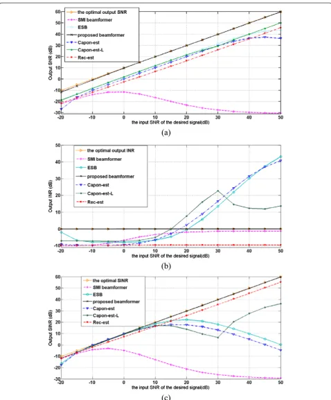
Example 3: The output SINR versus the desired signal SNR Recalling Equation (3), the following equation can be established the output SNR and output interference-to-noise ratio (INR) are defined as

INR versus different SNR of the desired signal are all given out. By observing these results, the process that the desired signal SNR how to affect the performance of each beamformer can be found out. Here, the look dir-ection is still randomly and uniformly distributed at [−2°,12°]. Hence, the random DOA mismatch of the

desired signal is still uniformly distributed in [−7°,7°]. The desired signal SNR varies from −20 to 50 dB. The snapshot number is assumed to be 500.

As deduced in the part 3, the proposed beamformer sup-presses the interference due to the fact that the steering vector of the interference is approximately orthogonal to Figure 1The beampattern of beamformers.

the reconstruction matrix R~f ¼R~−iþ1nR~s. For the optimal beamformer, the steering vector of the interference is ap-proximately orthogonal to the matrix R_f ¼R−1

iþnRs. It im-plies that the proposed beamformer and the optimal beamformer have nearly the same principle and ability of the interference suppression. The results in Figure 3b inves-tigate this saying. From Figure 3a, it can be found that the output SNR of the proposed one is quite close to the opti-mal beamformer in a large range from−20 to 50 dB. The optimal weight maximizing the output SINR can be consid-ered as a result of maximizing the output SNR under the premise of its approximately orthogonal to the steering vec-tor of the interference signal. The proposed weight is ob-tained by using the same scheme. Therefore, the proposed beamformer produce an output SNR quite close to the op-timal beamformer. As we know, the reconstructed matrix

~

Rs is constructed by using Capon spectral estimator inte-grated over regions where desired signals are located. Hence, when the SNR is very small, the spectral peak, ob-tained by using reconstructed matrix R~s, corresponding to the real DOA of the desired signal is quite flat. This causes an inaccurate estimate of the rotating vectorr, which leads to a slight worse result than the optimal beamformer. The joint action of the output SNR and the output INR results in that the proposed beamformer is always the closest one to the optimal SINR in a large range from −20 to 50 dB (see Figure 3c).

Because of the removing of the desired signal component from the covariance matrix, the output INR of the Rec-est. beamformer is not much sensitive to the desired signal SNR and can always follow the trend of the optimal beam-former. Moreover, the constraint of wHa^ ¼1 makes the value ofwHwvery small, which gives raise to that the out-put INR is smaller than the optimal beamformer and the proposed beamformer. However, due to the inaccurate esti-mation of the steering vector, the output SNR of the Rec-est. beamformer is inferior to the proposed one. Therefore, the final output SINR of the Rec-est. beamformer is smaller than the proposed one. The performance of the ESB, the Capon-est. beamformer and the Capon-est-L. beamformer can keep quite close to the optimal SINR in a range from −15 to 10 dB but degrade when SNR is higher than 20 dB. This is because their interference suppression becomes worse versus the increase of the SNR. For the SMI beam-former, as shown in Figure 3, the output SNR decreases and the output INR increases when the high desired signal SNR and large DOA mismatch appear at the same time. Thus, the performance of the SMI beamformer would de-grade versus the increase of the SNR.

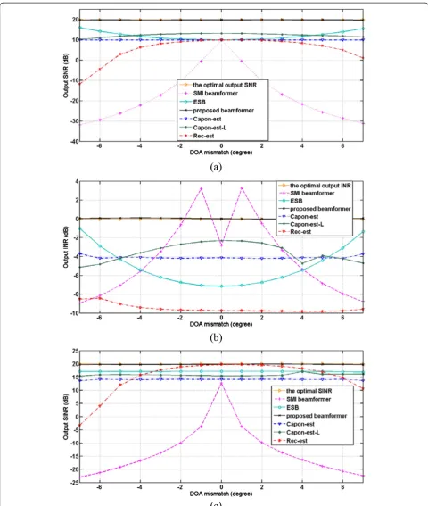
Example 4: The output SINR versus DOA mismatch In the last example, the output SINR of beamformers ver-sus different DOA mismatches is considered. Same with

example 3, the output SNR results and output INR results are also presented. SNR is assumed to be 10 dB and the number of snapshots is chosen as 200. The DOA mismatch is uniformly distributed at [−7°,7°]. Results are presented in Figure 4. As explained in example 3, the principle of obtain-ing the proposed beamformer imitates that of the optimal beamformer. When SNR = 10 dB, the proposed beamfor-mer has nearly the same output SNR and INR. Hence, it is easy to find that the proposed algorithm always provides an output SINR almost equal to the optimal value when DOA mismatch has a large uncertainty level. The Rec-est. beam-former is strongly affected by the DOA mismatch level and so does the SMI beamformer. For the Rec-est. beamformer, the imprecise estimation of the steering vector of the de-sired signal makes the output SNR small when the DOA mismatch level is large. For the SMI beamformer, the wrong constraint of wH_{a¼1 brings out a nulling in the} real DOA of the desired signal. Thus, the output SNR is quite small for large DOA mismatch level. The ESB, Capoon-est. beamformer, and Capoon-est-L. beamformer are not very sensitive to the DOA mismatch level. However, due to the constraint between the weight and the estimate steering vector of the desired signal, their output SNR is smaller than the optimal one and the proposed one. There-fore, their performance is inferior to the proposed beamformer.

5 Conclusions

A robust beamforming method based on the matrix struction is proposed. In this beamformer, two recon-structed matrices, the interference-plus-noise covariance matrix and the desired signal-plus-noise covariance matrix are used to replace their real sample covariance matrix, re-spectively. Then, an orthogonal subspace, orthogonal to the interference subspace and including the desired signal sub-space, can be obtained based on the principle of the output SINR maximization. Finally, an optimal weight vector can be found by maximizing the output power of the desired signal. This novel beamformer is able to always be a value nearly equal to the optimal value when DOA mismatch has a large uncertainty level and whenever the SNR level of the desired signal is low or high. Moreover, it has an excellent convergence rate. Numerical results demonstrate the effect-iveness of the proposed beamfomer compared with some of the existing ones.

Competing interests

The authors declare that they have no competing interests.

Acknowledgements

Received: 23 February 2014 Accepted: 27 May 2014 Published: 14 June 2014

References

1. M Wax, Y Anu, Performance analysis of the minimum variance beamformer. IEEE Trans. Signal Process.44(4), 928–937 (1996)

2. M Wax, Y Anu, Performance analysis of the minimum variance beamformer in the presence of steering vector errors. IEEE Trans. Signal Process.

44(4), 938–947 (1996)

3. HL Van Trees,Optimum Array Processing(Wiley, New York, 2002) 4. AB Gershman, Robust adaptive beamforming in sensor arrays. Int. J.

Electron. Commun.53, 305–314 (1999)

5. Y Han, D Zhang, A recursive Bayesian beamforming for steering vector uncertainties. EURASIP J Adv Signal Process.2013, 108 (2013) 6. DD Feldman, LJ Griffiths, A projection approach for robust adaptive

beamforming. IEEE Trans. Signal Process.42(4), 867–876 (1994) 7. BD Carlson, Covariance-matrix estimation errors and diagonal loading in

adaptive arrays. IEEE Trans. Aerosp. Electron. Syst.24(4), 397–401 (1988) 8. J Li, P Stoica, Z Wang, On robust Capon beamforming and diagonal

loading. IEEE Trans. Signal Process.51(7), 1702–1715 (2003)

9. SA Vorobyov, AB Gershman, ZQ Luo, Robust adaptive beamforming using worst-case performance optimization: a solution to the signal mismatch problem. IEEE Trans. Signal Process.51(2), 313–324 (2003)

10. RG Lorenz, SP Boyd, Robust minimum variance beamforming. IEEE Trans. Signal Process.53(5), 1684–1696 (2005)

11. JF Sturm, Using SeDuMi 1.02, a MATLAB toolbox for optimization over symmetric cones. Optimization Methods Software11–2(1–4), 625–653 (1999)

12. A Hassanien, SA Vorobyov, KM Wong, Robust adaptive beamforming using sequential programming: an iterative solution to the mismatch problem. IEEE Signal Process. Lett.15, 733–736 (2008)

13. A Khabbazibasmenj, SA Vorobyov, A Hassanien, Robust adaptive beamforming via estimating steering vector based on semidefinite relaxation, inProceedings of the 44th Asilomar Conference on Signals, Systems and Computers, ed. by SAM (Pacific Grove, CA, 2010), pp. 233–235 14. R Mallipeddi, JP Lie, PN Suganthan, SG Razul, CMS See, Robust adaptive

beamforming based on covariance matrix reconstruction for look direction mismatch. Progr. Electromagn. Res. Lett25, 37–46 (2011)

15. A Khabbazibasmenj, SA Vorobyov, A Hassanien, Robust adaptive beamforming based on steering vector estimation with as little as possible prior information. IEEE Trans Signal Process60(6), 2974–2987 (2012) 16. Y Gu, A Leshem, Robust adaptive beamforming based on interference

covariance matrix reconstruction and steering vector estimation. IEEE Trans. Signal Process.60(7), 3881–3885 (2012)

17. W Zhang, J Wang, S Wu, Robust Capon beamforming against large DOA mismatch. Signal Process.93(4), 804–810 (2013)

18. J Zhuang, A Manikas, Interference cancellation beamforming robust to pointing errors. IET Signal Process.7(2), 120–127 (2011)

19. M Grant, S Boyd, YY Ye, CVX: MATLAB software for disciplined convex programming, June 2014. http://cvxr.com/cvx/

20. RA Monzingo, TW Miller,Introduction to Adaptive Arrays(Wiley, New York, 1980)

doi:10.1186/1687-6180-2014-91

Cite this article as:Xieet al.:A robust adaptive beamforming method based on the matrix reconstruction against a large DOA mismatch.

EURASIP Journal on Advances in Signal Processing20142014:91.

_{Submit your manuscript to a}

journal and benefi t from:

7 Convenient online submission

7 Rigorous peer review

7 Immediate publication on acceptance

7 Open access: articles freely available online

7 High visibility within the fi eld

7 Retaining the copyright to your article