Spatial filter decomposition for interference mitigation

R E S E A R C H

Open Access

Spatial filter decomposition for interference

mitigation

Rabah Maoudj

, Michel Terre

, Luc Fety

, Christophe Alexandre

and Philippe Mege

Abstract

This paper presents a two-part decomposition of a spatial filter having to optimize the reception of a useful signal in the presence of an important co-channel interference level. The decomposition highlights the role of two parts of the filter, one devoted to the maximization of the signal to noise ratio and the other devoted to the interference cancellation. The two-part decomposition is used in the estimation process of the optimal reception filter. We propose then an estimation algorithm that follows this decomposition, and the global spatial filter is finally obtained through an optimal-weighted combination of two filters. It is shown that this two-component-based decomposition algorithm overcomes other previously published solutions involving eigenvalue decompositions.

Keywords:SIMO receiver; Optimum combining; Maximum ratio combining; Antenna array

1 Introduction

Increasing capacity demand for wireless communication networks should lead to a high co-channel interference level in the future. This interference problem is not new and has been addressed, for a long time, in wireless networks. The first solutions, coming from 2G networks, were based on frequency reuse patterns while, a few years later, scrambling codes were used, for the same purpose, in 3G networks. Nowadays, diversity techniques are more and more considered as one of the best answer for this interference problem, especially in 4G networks. The work presented in this paper was initially based on private mobile radio (PMR) characteristics linked to the TETRA enhanced data service (TEDS) standard, but it is suitable also in the context of 4G transmissions which are based on the Long-Term Evolution (LTE) standard. The presented work addresses essentially the problem of transmission with high interference level ratio and fast varying propagation channels.

In such a context, several previous works have treated and analyzed the best spatial filter to maximize the signal to interference plus noise ratio (SINR). The optimum combining (OC) filter [1-5] can be proposed as an exploitable solution. It was also proven that, in the absence of interference, this optimum combining

filter converges to the well-known maximum ratio combining (MRC) filter [6].

The main problem, in the estimation of the optimum combiner filter, resides in the estimation of the covariance matrix of the interference plus noise in addition to the estimation of the useful user propagation channel. The minimum mean square error estimation (MMSE) criterion can be used to estimate the desired user propagation chan-nel, while the covariance matrix can be estimated by the sample matrix inversion (SMI) approach [7-9]. However, this strategy is suboptimal and requires a large signal sample set to get a correct smoothing stage [10,11]. Another problem resides in the covariance matrix itself which will be obviously interpolated to the data locations since it is estimated on the pilot locations [10].

In this paper, we will prove that under certain condi-tions, the OC filter can perfectly be decomposed in two independent components. Hence, when the number of interferers is smaller than the number of receiving anten-nas, the OC filter can be split in two weighted components, namely MRC filter and interference canceller combiner (ICC). Moreover, for its own scientific interest, it will be proven that this decomposition leads to a new and efficient optimum filter estimation algorithm.

More precisely, we will show that for the MRC part of the OC filter, the classical MMSE can be proposed in order to obtain the estimation of the useful user propagation channel. On the other hand, we will show that the ICC part

* Correspondence:[email protected] 1_{CNAM/CEDRIC/Laetitia, Paris, France}

Full list of author information is available at the end of the article

can be estimated by modifying the matched desired impulse response (MDIR) algorithm [12]. This algorithm requires a null linear system solving, and a constraint is required to prevent the trivial solution. Following [12], a constraint, so-called maximum SINR constraint (MSINRC), can be introduced; it will maximize the SINR at the output of the filter. The final solution-vector will then be given by the eigenvector corresponding to the lowest eigenvalue of a Hermitian matrix generated by the algorithm. Due to the presence of the noise, the estimation still remains suboptimal and the result is corrupted by the training noise estimation. It was proven in [13] that combining all eigenvectors, weighted by the inverse of their correspond-ing output SINR, could lead to an enhanced algorithm, so-called solution-vectors maximum ratio combining (SoMRC). It was shown that this approach gives better performance than the single solution-vector [13,14]. Obvi-ously, such kind of algorithms is based on a complex eigendecomposition. To simplify this step, we propose to introduce another constraint, leading to a less complex algorithm where we can avoid the eigendecomposition. We will also show that this new constraint keeps the performance of the algorithm comparable to that of the SoMRC.

The contribution of the presented work in the study of the optimum combiner filter consists on identifying the cases where it can be decomposed to a MRC plus a ICC independent filters. Another contribution consists of the modified MDIR algorithm and in the introduction of the new constraint that does not degrade performances of the SoMRC. A 16-bit digital signal processor (DSP) implementation is also presented in order to evaluate the rounding errors effect on the performance of the algorithm and to determine the possibility of the algorithm execution under some real-time constraints.

The paper is organized as follows. The system model is given in Section 2. Section 3 presents the split of the OC into two weighted independent parts, namely MRC and ICC. In Section 4, the estimation algorithm for ICC is detailed. A simplification of this estimation algorithm is introduced in Section 5. Numerical results and per-formance of the algorithms are presented in Section 6. A performance degradation study, due to a practical 16-bit fixed point DSP implementation is detailed in Section 7. Conclusion summarizes the present work in Section 8.

1.1 Notation

Vectors and matrices are boldface small and capital letters; the transpose, complex conjugate transpose, and inverse of matrixAare denoted byAT,AH, andA−1, respectively.

The norm of vectoraand the diagonal matrix with the diagonal element extracted from a are denoted respect-ively by ‖a‖ and diag{a}, IN is theN × N identity matrix, andE[.] denotes the statistical expectation.

2 System model

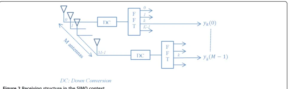
We consider a SIMO structure havingM receiving anten-nas, with one desired signal andUinterferers, as presented in Figure 1. Desired user and interferers are transmitting orthogonal frequency-division multiplexing (OFDM) wave-forms, and for the sake of simplicity, we will consider that all users are time and frequency synchronized. This remark is not restrictive, and all results presented are not linked to this hypothesis that will nevertheless simplify some notations in the sequel of the paper.

The OFDM frame of the desired user is composed of

Ksubcarriers andNsOFDM symbols. ANglength cyclic prefix is inserted. It is assumed that this cyclic prefix is sufficient to totally suppress intersymbol interferences. We will focus on one OFDM symbol, and we will avoid indicating the symbol number in the notations. Algo-rithms presented will then be able to cope with a unique OFDM symbol and therefore able to deal with very high-speed propagation channels.

With this assumption, the received sample, after the OFDM demodulation, corresponding to thekth subcarrier on the mth antenna, as presented in Figure 2, can be modeled by Equation 1:

y_kð Þ ¼m hx;kð Þm xkþnIkð Þm ð1Þ

nI

kð Þm denotes an additive noise plus interference term and can be developed as follows

nI_kð Þ ¼m XU

u¼1hz;k;uð Þmzk;uþnkð Þm ð2Þ

Zk,uis the symbol transmitted by theuth interferer.

hz,k,u(m) denotes the frequency response of the channel between the uth interferer and the mth antenna. nk(m) represents a centered additive white Gaussian noise term

with a variance equals toσn2.

XU

u¼1hz;k;uð Þm zk;uis then the total contribution of the U interferers received by the mth antenna on the kth subcarrier.

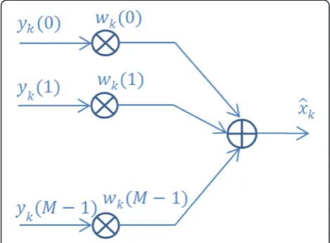
In this paper, we have to identify a spatial filterwkable to estimate the QAM symbol ^xk transmitted by the desired user. This leads to

^

xk ¼wHkyk ð3Þ

In this equation, corresponding to the kth subcarrier,

wk¼

A denotes, as illustrated in Figure 3,

M weights of the spatial filter and y_k¼

y_kð Þ0

ofM antennas. Combining Equations 1, 2, and 3 leads to Equation 4

^

xk ¼wHk hx;kxkþ

XU

u¼1hz;k;uzk;uþnk

ð4Þ

where hx;k¼

hx;kð Þ0

⋮

hx;kðM−1Þ

0 @

1

A denotes the M desired propagation channel frequency responses of the kth subcarrier,

hx;k;u¼

hx;k;uð Þ0

⋮

hx;k;uðM−1Þ

0 @

1

A the M interfering propaga-tion channel frequency responses between the uth in-terferer and the receiving antennas, and finally

nk ¼

nkð Þ0

⋮

nkðM−1Þ

0 @

1

A stands for the received noise on the

Mreceiving antennas.

The spatial filter that maximizes the signal to interfer-ence plus noise ratio (SINRk) for ^xk was introduced in

[1] and studied in [2,3]. Main steps of this derivation are presented hereafter.

We could consider, without loss of generality, that

E[|xk|2] = 1 andE[|zk,u|2] = 1. According to Equation 4, the SINRk, at the output of the spatial filter, is then given by

SINRk¼

wH

kh

x;khTx;kwk

wH

kRnn;kwk

ð5Þ

In this equation, Rnn,k stands for the M × M spatial covariance matrix of interference plus noise, and it is expressed by

Rnn;k¼E XU

u¼1

hz;k;uzk;uþnk !

XU

u¼1

hz;k;uzk;uþnk !H

" #

ð6Þ

Considering the decorrelation between interferer signals and noise terms, we have

Rnn;k¼XU

u¼1E h

z;k;uhTz;k;u

h i

þσ2

nIM ð7Þ

By introducing theRzz,kmatrix defined by Figure 1Context of the work, one useful user, andUinterferers.

Rzz;k¼XU_u¼1E hz;k;uhT_z;k;u

At the output of the combiner, in order to perfectly equalize the useful channel, we propose to introduce the following constraint

wH

kh

x;k¼1 ð10Þ

Merging Equations 5 and 9, the SINRkbecomes

SINRk¼

1

wH

kRnn;kwk

ð11Þ

The optimum spatial filter vector wk that maximizes the SINRk can then be obtained by minimizing wH_kRnn;k

wk under the constraint wHkh

x;k¼1 . Using Lagrange multiplier, the optimum spatial filter is obtained by solving the following equation

wk¼ arg minL 1

SINRk;wk;λ

ð12Þ

where the Lagrangian is defined such that

L 1

Under the assumption that det d

2_L 1 the solution is obtained by nulling the derivative of

L 1

SNIRk;wk;λ

with respect to wk

dL 1

SINRk;wk;λ

dwk ¼0 ð14Þ

Solving Equation 14 leads to

Rnn;kwk−λh

x;k¼0 ð15Þ

The optimal [1] solution is then expressed by

wk¼λR−1

nn;khx;k ð16Þ

The minimum of the solution (Equation 12) is justified by the positive Hermitian characteristic of the covariance matrixRnn,k. We have

Identifying the spatial filterwkthrough Equation 19 is a very complex task involvingRnn,kestimation and inversion plushx,k estimation. In order to address this spatial filter estimation problem, we propose to split it on two sepa-rated filters. This approach highlights how the optimal spatial filter works.

3 Spatial filter decomposition

We consider the eigenvector matrix Uk and the diag-onal matrix I_μk of the eigenvalues defined such that

Iμk¼

A. Then, the eigenspace de-composition ofRzz,kcan be written as follows

Rzz;k¼UkIμkU

H

k ð20Þ

According to the Rnn,k decomposition, presented in Equations 7 and 8, we obtain

Rnn;k¼UkIμkþσ2nU the transpose adjugate (cofactor) matrix of Rnn, defined as follows

R−1

nn;k¼_detCnn;k_Rnn;k ð22Þ

Replacing R−_nn1_;k by Cnn;k

detðRnn;kÞ in the denominator of

Equation 19 leads to

wk¼

stands for a

diag-onal matrix such that itsmth component is given by YM−1

Then, Equation 24 can be rewritten as follows

detRnn;kR−1nn;k ¼Czz;kþσn2ðM−1ÞIþGm;k ð25Þ

where Gm,k is null matrix for M≤2 otherwise is de-fined by the following expression

Gm;k¼

As shown in the previous equation, Gm,k is linked to the interference covariance matrix. We note that in the case of totally decorrelated interferers,Rzz;k ¼σ2cI.

Finally, we obtain the following decomposition of the spatial filterwk

wk¼

We conclude that the optimal spatial filter is a combin-ation of three filters: mainly a filter dedicated exclusively to the interference, a maximum ratio combiner filter, and a filter linked to the statistical dependency of the interferers. Due to the complexity of the third filter, the estimation of the optimal spatial filter through the sep-arate estimation of the filters is only interesting in the case of a two-antenna receiver (Gm,k=0).

3.1 Analysis forM= 2

If we consider now a two-antenna spatial filter (M= 2), in this case, the optimal spatial filter given by Equation 27 becomes From Equation 24, we have

Cnn;k¼UkIY _μþσ2

Replacing Equation 30 in Equation 28, we obtain

wk¼

We introduce now theρkscalar defined as follows

ρk¼

hH_x;kCzz;khx;k

hH_x;khx;k ð32Þ

After some derivations, we arrive to

wk¼

This equation can be presented as follows

wk¼

Equation 34 expresses the optimum combiner wk through a weighted combination of two combiners wz,k andwh,k.

From this observation, we can derive the following theorem.

Theorem: In the case of two-antenna SIMO receiver, the optimum combinerwkcan be expressed as a weighted

combination of the optimum combiner wz,k obtained in

the case of null additive white Gaussian noise and the maximum ratio combinerwh,k.

Furthermore, of the physical interpretation of the optimal spatial filter, this decomposition can also be used to esti-mate the optimal spatial filter in two steps: a step devoted to the optimum combiner without taking into account the additive noise wz,k and the other to the maximum ratio combinerwh,k.

4 Spatial filter estimation 4.1 Estimation algorithm forwh,k

Thewh,kfilter does not depend on interference but only on the desired signal propagation channel. Its estimation is then directly linked to the estimation of the propagation channelhx,k.

In this work, we consider that propagation channels, i.e., useful and interference channels, can be modeled asLtaps finite impulse response filters and withL<K. We introduce then these impulse responses, corresponding to themth antenna, through the following vectors

axð Þ ¼m

Thanks to this hypothesis we can introduce the hx(m) vector that represents the frequency response of the propagation channel between the useful user and the

mth antenna

where FK,L is the K×L truncated Fourier rectangular

matrix defined as follows

FK;Lðk;lÞ ¼ 1ffiffiffiffi

In the context of a real transmission, a first estimation ~

hxð Þm of hx(m) can be proceeded through the classical least square as given in the following equation

~ great number of observations, they are highly imprecise and they depend on the additive noise over the yk(m) received samples. A smoothing operation [15], leading to a new estimated ^hxð Þm vector, can be proposed through the following equation

^

hxð Þ ¼m FK;LFHK;L^hxð Þm ð42Þ

This estimation algorithm is known as the indirect esti-mation [16,17], and some papers [18] propose to enhance it through the introduction of a noise power estimation and an adaptive weight, able to take this estimation into consideration.

The main drawback of this algorithm comes from Equation 41 that involves knowledge of all transmitted symbols {xk}k∈[0,K−1]. In a real transmission, only pilot symbols are known. If we consider that we have K′<K

comb pilots {x0′,x1′,…,xK′}, then Equation 41 becomes

estimation of the propagation channel frequency responses on the pilot locations.

The first estimation for the propagation channel impulse response can then be obtained through

~

axð Þ ¼m FHK′;L~h′xð Þm ð44Þ

Then, an interpolation step is required. It is performed by the following equation

^

hxð Þ ¼m FH_K′;L~h′xð Þm ð45Þ

Equation 45 is devoted to themth antenna, and it can be generalized to all antennas. If we consider now the

kth component h^x;kð Þm of all these ^hxð Þm

n o

^

4.2 Estimation algorithm forwz,k

Thewz,kvector is jointly dependent on interference, and propagation channels are devoted to interference sources cancellation. It is well known that a M antenna spatial filter is able to cancel U=M−1 interferers. In our par-ticular case, where we chooseM= 2, we have then to cope with a unique interferer. In the sequel of this section, the

uindex that represents the interferer index will be omitted in equations.

We consider the transmission of a unique OFDM symbol, the eigendecomposition ofRzz,kis given by

Rzz;k ¼Uk μ₀0;k 0₀

UH_k ð48Þ

And the eigendecomposition of Czz,k is given as follows

where μ2,k is the second column vector of Uk

orthog-onal to the interference vector hz;kð Þ0

hz;kð Þ1

. Therefore,

the following scalar vector is null uT 2;k

The filterwz,kwill then be rewritten as

wz;k¼ μ0;ku2;ku

Finally, the solution is given by

wz;k¼wz;k;n

The positive scalar ρk in the general formula of the optimal spatial filter given in Equation 34 becomes

ρk¼μ0;k

uH_2;khx;k2 hx;k2

ð54Þ

Therefore, ρk is the intercorrelation factor between the desired and the interference channel vectors. From the theorem stated above and Equation 50, we emit the following proposition.

Proposition:In the case of two-antenna SIMO transmis-sion disturbed by an interferer,the optimum combinerwkis

a weighted combination of the interference cancellation filter

wz,kand the maximum ratio combining filterwh,k.

The estimation of wz,k,n and wz,k,d is a complex task that involves the knowledge of the desired and interferer propagation channels. Nevertheless, the expression ofwz,k,n andwz,k,dgiven by Equations 52 and 53, respectively, gives opportunities to project these components on a reduced Fourier basis.

4.2.1 wz,k,nestimation

On the first hand, we can notice that the components of wz,k,n are simply those of the frequency response of the interferer propagation channels, corresponding to the kth subcarrier. Therefore, the components of this filter can then easily be expressed on a reduced Fourier basis. For that purpose, we introduce the (K× 1), hz(m) vector that represents the frequency response of the propagation chan-nel between the interferer and themth antenna as follows

hzð Þ ¼m theL taps impulse responseaz(m) through the following equation

Therefore,wz,ncan be expressed as

wz;n¼FK;Lvz;n ð58Þ

4.2.2 wz,k,destimation

If we introduce the (2L× 1) vz,d vector representing this virtual impulse response

vz;d¼

vz;0;d

⋮ vz;2L−1;d

0 @

1

A ð59Þ

Then we can introduce thewz,dvector defined as

wz;d¼

wz;0;d

⋮ wz;K−1;d

0 @

1

A ð60Þ

with

wz;d¼FK;2Lvz;d ð61Þ

4.2.3 Replica spatial filter structure

The decomposition of wz,k in a numerator part and a de-nominator part as given by Equation 51 leads to propose a new spatial filter structure having two weights, represented bywz,k,nacting over the received signal and a weight, repre-sented bywz,k,d,acting over the useful signal (Figure 4).

We can then introduce the errorekdefined by

ek¼wz;k;dxk−½ykð Þ0 ykð Þ1 wz;k;n ð62Þ

At this stage, knowing that the wz,kfilter has to cancel the interference, we can propose to identify its two com-ponents through an error square minimization criterion

wz;k¼ arg min

wz;k;n;wz;k;d

ek

j j2 _ð63Þ

We have then to insert a constraint ψ(wz,k,n, wz,k,d ) in order to avoid the trivial solution: (wz,k,n= 0, wz,k,d= 0). Moreover, the minimization has to be done over all fre-quencies. It is then necessary to propose a global criterion. For that purpose, we introduce theXtransmitted diagonal data matrix, where each element xk corresponds to the desired symbol transmitted over thekth subcarrier

X¼diagfx0;x1;…;xK−1g ð64Þ

We introduce also the bi-diagonal matrix Y of the received signal over the two antennas

Y¼

y₀ð Þ0 0 0

0 ⋱ 0

0 0 y_K−1ð Þ0

y₀ð Þ1 0 0

0 ⋱ 0

0 0 y_K−1ð Þ1 0

@

1 A

ð65Þ

The e¼

e0

⋮

eK−1

0 @

1

A vector representing errors over all subcarriers is then given by

e¼Xwz;d−Y wz;n ð66Þ

The filter weights are then given by the following minimization

wz¼ arg min wz;d;wz;n

e2−μψwz;n;wz;d

ð67Þ

whereμis a Lagrange multiplier.

In [12,19] and in a similar context, a constraint called maximum signal to interference plus noise constraint (MSINRC) is proposed. It is defined as

ψwz;n;wz;d ¼ Xwz;d 2−1 ð68Þ

Without loss of generality, we can consider that all transmitted symbolsxkare normalized: |xk|2= 1, we have then XH X=I. The constraint presented in Equation 68 is then equivalent to‖wz,d‖2= 1.

By nulling the partial derivative of ‖e‖2−μψ(wz,n,wz,d) with respect towz,nandwz,d[20], we obtain the following system of equations

XHY wz;n−wz;d¼μwz;d

wz;n¼YHY−1YHXwz;d

(

ð69Þ

Merging the two equations of Equation 68, we arrive to

XH Y Y HY−1YH−I

Xwz;d¼μwz;d ð70Þ

It appears then that wz,d is the eigenvector of the

XH

(Y(YHY)−1YH−I)X matrix corresponding to the μ eigenvalue.

Left multiplying the two sides of Equation 70 by wH

This last equation leads to

1

In the right side of Equation 72, we recognize the SINR formula; we can then conclude that

1

μ¼SINR

Finally, as we have to maximize the SINR at the output of the filter, wz,d has to be the generalized eigenvector which corresponds to the minimal eigenvalue μ. Using Equation 61, Equation 72 becomes

XH Y Y HY−1YH−I

XFK;2Lvz;d¼μFK;2Lvz;d ð73Þ

Left multiplying the two sides of this equation by

FH

K;2Lyields to

F_K;H_2LXHY Y HY−1YH−IXFK;2Lvz;d¼μvz;d ð74Þ

It appears that from Equation 74, the virtual impulse response Vz,d is the (2L× 1) eigenvector of the matrix

XFK;2Lcorresponding to the minimal eigenvalueμ. This result is known and used by many authors. An enhanced maximum signal to interfer-ence plus noise constraint (EMSINRC) is proposed in [13]. It is based on the exploitation of the setVz,dof all the eigenvectors of the previous matrix defined as

Vz;d¼ v0z;d … v2z;dL−1

ð75Þ

The EMSINRC algorithm introduces a linear combin-ation of elements ofVz,d, in order to propose a composite virtual impulse responsevc

z;ddefined as follows

vc_z;d¼X

where μi is the eigenvalue corresponding to the eigenvector vi_z;d. The complex term ηiis defined such scalar is acting as a phase term that aligns all eigenvectors.

Concerning the vector vz,n, it is obtained by merging Equation 58 into the second equation of the system (69). Hence,vz,nis given as follows forming Equations 61 and 58, respectively, the interferer cancellation filterwz;k¼w_wzz;_;kk_;;n_dfor all subcarriers is obtained. At this stage, all elements have been established and the optimal filter, given by Equation 34, can be estimated. The combination of Equation 34 is based onρkthat can be obtained directly from Equation 54 noticing that the interferer power μ0 and σ2

n can be obtained through a noise plus interferer power estimation.

5 Interference cancellation filter simplification

The estimation of wz,d and wz,n involves an eigende-composition which is a complex task, especially if we consider a practical implementation of the algorithm in the real-time context of the receiver. We will show, in this section, how this eigendecomposition can be avoided without involving any loss in the global performances of the algorithm.

The key element comes from the constraint introduced to avoid the trivial solution. Instead of ‖wz,d‖2= 1, we propose to introduce a constraint directly applied to the virtual impulse response vz,d. This constraint consists in forcing a component of this vector to be equal to 1.

If we denote by kb, the index of this component, the constraint will be then given byvz,d(kb) = 1.

We will introduce now a square matrixB, with all zero components except a diagonal component set to 1; the constraint is then formalized as follows

Bvz;d¼1kb ð78Þ

where 1kb is a vector whose all components are null exceptkth_b component set to 1. The constraint can then be formalized with the following functionψ′(vz,d)

ψ′vz;d¼ Bvz;d 2−1 ð79Þ

The interference cancellation filter weights are then given by the new following minimization

vz;n;vz;d

The derivation of Equation 80 with respect to vz,d leads to the new solution (v′z,n,v′z,d) given by

v′z;d−FHK;2LXHY FKK;LLv′z;n−μ′BHBv′z;d¼0 ð81Þ

v′z;d−FHK;2LX H_{Y F}

KK;LLv′z;n−μ1kb¼0 ð82Þ

The derivation of Equation 80 with respect to vz,n leads to

−FH_KK;LLYHXFK;2Lv′z;dþFHKK;LLYHY FKK;LLv′z;n¼0

ð83Þ

By developing Equation 83, we obtain

v′z;n¼ FHKK;LLYHY FKK;LL

−1

FH_KK;LLYHXFK;2Lv′z;d

ð84Þ

Merging Equation 84 in Equation 82, we obtain

FH_K;2LXHI−Y Y HY−1YHXFk;2Lv′z;d¼μ′1kb ð85Þ

This last equation can be rewritten as

v′z;d¼μ′Ω−11kb ð86Þ

withΩ¼FH

K;2LXH I−Y YHY

−1

YH

XFK;2Land where

μ′is a scalar chosen such thatv′z,d(kb) = 1.

Finally, the solution obtained from the proposed con-straint leads to a solution given by Equations 84 and 86. With these two equations, the eigendecomposition is avoided and the implementation complexity is widely reduced. The question of the optimality of this new solution has then to be analyzed in details. For that purpose, we propose to decompose the vector v′z,d in the Vz,d orthogonal basis introduced in Equation 75. We can then define a (2L× 1) vector αd representing the image ofv′z,din theVz,dbasis as hereafter

v′z;d¼Vz;d

α

AsVz,dare eigenvectors of theΩmatrix, we have

Ωv′z;d¼Vz;dIμαd ð88Þ

whereIμis the diagonal matrix of eigenvalue ofΩ.

Considering Equation 86, theαdvector is then given by

αd¼I−1μVHz;dμ′1kb ð89Þ

Finally, Equation 89 becomes

v′z;d

X2L−1 i¼0 η′i

1 μi

vi

z;d ð90Þ

where η′iis theith component of the kth_b column vector

of the matrixVH z;d.

This last equation has to be compared to Equation 76 related to the EMSINRC algorithm. It leads to the conclusion that the EMSINRC algorithm is in fact equivalent to a constraint modification leading to a new constraint given by Equation 79.

6 Simulation results

In this section, we first evaluate performance of the vari-ous solutions presented in Sections 4 and 5. We will then compare:

– The solution based on (vz,n,vz,d) that will be referred

as maximum signal to interference plus noise ratio constraint (MSINRC)

– The solution based on vc

z;n;vcz;d

that will be referred as enhanced maximum signal to

interference plus noise ratio constraint (EMSINRC)

– The solution based on (v′z,n,v′z,d) that will be

referred as coefficient constraint (CC)

Table 1 OFDM parameters

Symbol Name Value

K Number of subcarriers 32

NFFT FFT size 32

Ncp Cyclic prefix NFFT

8 ¼4

W Total bandwidth 100 kHz

Δf Subcarrier spacing 3,125 kHz

TOFDM OFDM symbol duration 360μs

TFrame Frame duration 18.36 ms

Figure 5Pilots distribution over the OFDM symbol.

The simulation parameters based on OFDM waveform are summarized in Table 1, hereafter.

The modulation used is 4-QAM with the same

power for pilots and data. The propagation channels used follow the Jakes model [21] with a propagation channel impulse response described in GSM standard [22], namely TU50 (typical urban with a mobile vel-ocity of 50 km/h) and HT200 (hilly terrain with a mobile velocity of 200 km/h). The pilots are uniformly distributed along the frequency axis with a rate of 1

2as depicted in Figure 5 and along the time axis with a rate of1

5.

Algorithm's weights are estimated on the plots position for each OFDM symbol containing pilots. An interpolation within the subspace generated by the reduced DFTFLand

F2Lis followed to extend the weights to the whole OFDM symbol.

However, along the time axis, the interpolation method used is the spline cubic [23].

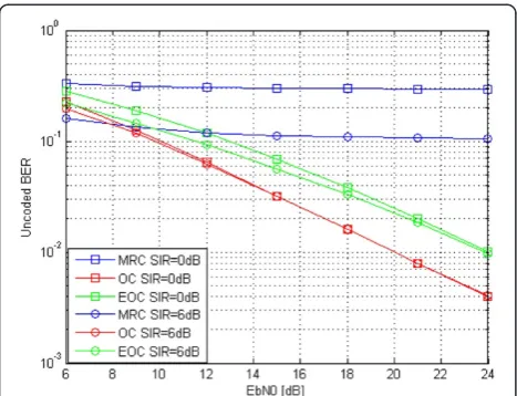
Performance assessment is performed by comparing the uncoded BER (bit error rate before channel decoding) vs.

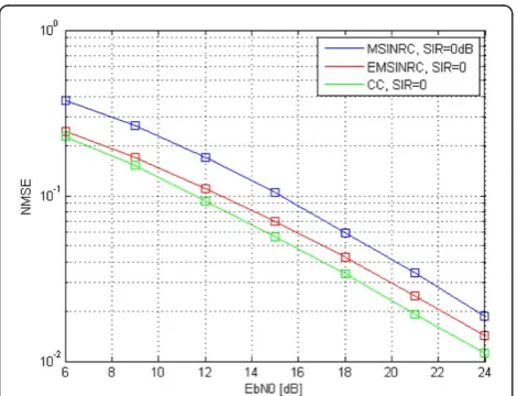
EbN0(signal to noise ratio) at signal to interference ratio (SIR) equal to 0 and 6 dB. As in [24,25], an additional comparison is done to confirm the previous one and con-sists on the study of the normalized mean square error

(NMSE) of^v expressed as NMSE¼k^v−vk v

k k2 2

;where vis the exact weight vector cancelling totally the interference, and

^

v¼ ^vn

^ vd

is the estimation of v using the constraints

studied in Section 4.

Figure 8Replica spatial filter structure NMSE ofvfor various constraints in TU50 channel propagation environment.

Figure 9Replica spatial filter structure NMSE ofvfor various constraints in HT200 channel propagation environment.

Figure 10BER performance of EOC vs. MRC and OC in TU50 channel propagation environment.

Figures 6 and 7 depict the uncoded BER obtained for the different constraints used in the weight vector estimation^v. The observation of the curves confirms the theoretical ana-lysis where the CC outperforms the MSINRC in the both cases of propagation channel environment. The difference in the performance is more pronounced for lowEbN0level, and obviously, the curves converge when EbN0 becomes high. Moreover, as expected in the theoretical analysis, the curves of CC and EMSINRC are superposed.

We conclude that CC is not only the best choice in the sense of bit error rate performance but also achieves very low complexity in its implementation. As shown in Equation 90, the solution is obtained by a simple matrix inversion unlike the other methods which need an eigendecomposition.

This difference of BER performance between the con-straints studied in Section 5 is confirmed by the NMSE as depicted by Figures 8 and 9. It is clearly shown that for CC constraint, the NMSE is less important than the MSINRC and close to the EMSINRC.

In the sequel, we discuss the performance of the esti-mated optimum combiner (EOC) based on the weighted combination of the estimated replica spatial filter using CC and the estimated MRC. EOC is then compared to the exact MRC (propagation channel hd is perfectly

known) and the exact optimum combiner (OC) where the covariance matrixRnnand propagation channelhdare perfectly known. Furthermore, additive white Gaussian noise (AWGN) power is assumed known.

Figures 8 and 9 show that the EOC in TU50 propaga-tion environment is better than in HT200 condipropaga-tions. In TU50, the EOC presents a good performance com-paring to OC, and there is only 2 dB of difference at

EbN0= 20 dB. However, in HT200 environment, this difference is more significant and is approximately about 4 dB atEbN0= 20 dB. This degradation is attributed to the estimation error of the EOC, which is proportional to the size of the weight vector. For example, in our case, the total weight vector length is equal to 4LTU= 8 for TU50 and 4LHT= 12 for HT200. We denote by LTU= 2 andLHT= 3 the maximum impulse response length of the propagation channels in TU50 and HT200 environments, respectively (Figures 10 and 11).

Table 2 Execution time and memory use

Step Memory used

[bytes]

DSP cycle count

Execution

time (μs)

Weights estimation (with Gauss)

2,348 1,859,684 1,860

Gauss (with prescaling) 420 84,770 (97,205) 84

Cholesky (with prescaling) 1,280 70,306 (83,777) 70

Channel equalization 28 458,725 458

Figure 11BER performance of EOC vs. MRC and OC in HT200 channel propagation environment.

Figure 12BER performance replica filter on 16-bit fixed point in TU50 channel propagation environment.

7 Real-time implementation

The complexity of an algorithm is often quantified in terms of the number of arithmetic operations. This quan-tification provides an estimate of the use of memory and execution time necessary to execute the algorithm.

Generally, algorithms are designed for real-time use and have to be performed by finite precision processors then the study of complexity raised above can meet the first requirement, but not enough to satisfy the second. In this section, we have performed a 16-bit DSP imple-mentation in order to insure a full analysis, namely to check that the real-time constraint and 16-bit fixed points degradation tolerance are respected.

EOC using CC constraint is implemented into the 16-bit fixed-point DSP (TMS 320C6474) which works at frequency clock of 1G Hz [26]. The whole of the receive chain is implemented, but we will show only the results of the part where the discussed algorithms are involved, namely the channel equalization.

Table 2 shows the execution time and memory uses performance of the algorithm. The main complexity cost in the EOC algorithm steels the relatively high dimension matrix to be inverted. Two methods of matrix inversion are implemented, namely Gauss-Jordan and Cholesky decomposition. The difference in the sense of execution time is negligible. The total execution time for the channel equalization is 210.7 μs per OFDM symbol which represents 1.15% of the frame duration.

The degradation caused by the 16-bit fixed-point format over the full precision floating point is shown in Figures 12 and 13 for TU50 and HT200 environments, respectively. These results are given in terms of uncoded BER vs. signal to interference ratio (SIR) at EbN0= 20 dB. One can observe that we have obtained satisfactory results in both cases of Gauss and Cholesky implementation.

8 Conclusions

This paper presents a new expression for the optimum combining filter for the case of a two-antenna based receiver. This expression is a weighted combination of two components. The first component is the combiner obtained in the case of null additive white Gaussian noise and the second is the combiner obtained in the case of null interference. This decomposition is important because it allows the optimal combining estimation through two filters of known sizes, so the problem of the size of the filters is avoided. A detailed study dedicated to a SIMO transmission in the case of one interferer and two receive antennas is presented in order to confirm the importance of this decomposition. A DSP implementation is also investigated to quantify the algorithm complexity. The success of this implementation is a proof that this algorithm is ready to use at least in cases close to the given example.

We note that all developments presented in the estima-tion part of the OC study have been based on one dimen-sion estimation, mainly the frequency axis of the OFDM frame. However, the proposed method can be done on the time axis of the frame such as in [27,28] or on both axis.

Competing interests

The authors declare that they have no competing interests.

Author details

1_{CNAM/CEDRIC/Laetitia, Paris, France.}2_{Airbus Group, Elancourt, France.}

Received: 28 March 2014 Accepted: 29 July 2014 Published: 15 August 2014

References

1. GG Raleigh, JM Cioffi, Spatio-temporal coding for wireless communication. IEEE Trans. Commun.46, 357–366 (1998)

2. Z Tang, RC Cannizzaro, G Leus, P Banelli, Pilot-assisted time-varying channel estimation for OFDM systems. IEEE Trans. Signal Process.55(5), 2226–2238 (2007) 3. AJ Baird, CL Zahm, Performance criteria for narrowband array processing.

Proc. IEEE Conf. Decis. Control.1, 564–565 (1971)

4. Y Zhihang, J MinChul, K Il-Min, Outage probability and optimum combining for time division broadcast protocol. IEEE Trans. Commun.10, 1362–1367 (2011) 5. JH Winters, Optimum combining in digital mobile radio with cochannel

interference. IEEE J. Selected Areas Commun.2, 528–539 (1984) 6. S Roy, P Fortier, Maximal-ratio combining architectures and performance

with channel estimation based on a training sequence. IEEE Trans. Wireless Commun.3, 1154–1164 (2004)

7. Y Hara, Weight-convergence analysis of adaptive antenna arrays based on SMI algorithm. IEEE Trans. Wireless Commun.2, 56–57 (2003)

8. LL Horowitz, H Blatt, WG Brodsky, Controlling adaptive antenna arrays with the sample matrix inversion algorithm. IEEE Trans. Aerosp. Electron. Syst.

15, 840–848 (1979)

9. J Ketonen,Equalization and Channel Estimation Algorithms and Implementations for Cellular MIMO-OFDM Downlink(University Of Oulu, Oulu, Finland, 2012) 10. I Barhumi, G Leus, M Moonen,MMSE Estimation of Basis Expansion Models

for Rapidly Time-Varying Channels(ESAT laboratory of the Katholieke Universiteit Leuven, Leuven, Belgium, 2005)

11. S-H Lee, H-S Kim, Y-H Lee, Complexity reduced space ML detection for other-cell interference mitigation in SIMO cellular systems. Eur. Trans. Telecom.

22(1), 51–60 (2011)

12. MA Lagunas, J Vidal, AI Pérez Neira, Joint array combining and MLSE for single-user receivers in multipath gaussian multiuser channels. IEEE J. Selected Areas Commun.18(11), 2252–2259 (2000)

13. J Vidal, M Cabrera, A Augustin, Full exploitation of diversity in space-time MMSE receivers. IEEE Vehicular Tech. Conf.5, 2497–2502 (2000) 14. R Maoudj, M Terre, Post-combiner for interference cancellation algorithm.

Int. Conf. Softw. Telecomm. Comput. Netw.1, 1–5 (2012)

15. C Dumard, T Zemen, Low-complexity MIMO multiuser receiver: a joint an-tenna detection scheme for time-varying channels. IEEE Trans. Signal Process.56(7), 2931-2940 (2008)

16. P Hoeher, S Kaiser, P Robertson, Pilot-symbol-aided channel estimation in time and frequency. IEEE Global Telecom. Conf. GLOBECOM 90–96 (1997) 17. G Auer, E Karipidis, Pilot aided channel estimation for OFDM: a separated

approach for smoothing and interpolation. IEEE Trans. Commun.

4, 2173–2178 (2005)

18. F Salman, J Cosmas, Y Zhang,Pilot aided channel estimation for SISO and SIMO in DVB-T2 (Annual post graduate symposium on the convergences of telecommunication, networking and broadcasting(Liverpool, England, 2012), pp. 1–6

19. M Caus, A Perez-Neira, Space-time receiver for filterbank based multicarrier systems, inProcedure of international ITG workshop on Smart Antennas WSA (Bremen, Germany, 2010), pp. 421–427

20. H Wen-Sheng, C Bor-Sen, ICI Cancellation for OFDM communication systems in time-varying multipath fading channels. IEEE Trans. Commun.

4(5), 2100–2110 (2005)

22. COST-207,Digital land mobile radio communications(Final report of the COST-project 207, Commission Of the European Community, Brussels, 1989) 23. SA Dyer, JS Dyer, Cubic-spline interpolation. 1. IEEE Instrum. Meas. Mag.

4(1), 44–46 (2001)

24. MR Raghavendra, S Bhashyam, K Giridar, Interference rejection for parametric channel estimation in reuse-1 cellular OFDM systems. IEEE Trans. Vehicular Tech.58, 4342–4352 (2009)

25. T Zemen, CF Mecklenbräuker, J Wehinger, RR Müller, Iterative joint time-variant channel estimation and multi-user detection for MC-CDMA. IEEE Trans. Commun.5, 1469–1478 (2006)

26. TMS320C6474 Multicore digital signal processor data manual (Rev. H) (Texas Instruments Incorporated, 2001)

27. T Zemen, CF Mecklenbrauker, Time-variant channel estimation using discrete prolate spheroidal sequences. IEEE Trans. Signal Process.

53, 3597–3607 (2005)

28. T Zemen, L Bernado, N Czink, Iterative time-variant channel estimation for 802.11p using generalized discrete prolate spheroidal sequences. IEEE Vehicular Tech. Conf.1, 1222–1233 (2012)

doi:10.1186/1687-6180-2014-127

Cite this article as:Maoudjet al.:Spatial filter decomposition for interference mitigation.EURASIP Journal on Advances in Signal Processing 20142014:127.

Submit your manuscript to a

journal and benefi t from:

7 Convenient online submission

7 Rigorous peer review

7 Immediate publication on acceptance

7 Open access: articles freely available online

7 High visibility within the fi eld

7 Retaining the copyright to your article