Two types of co-accretion scenarios for the origin of the Moon
Ryuji Morishima and Sei-ichiro Watanabe
Department of Earth and Planetary Sciences, Nagoya University, Nagoya 464-8602, Japan
(Received May 24, 2000; Revised October 19, 2000; Accepted December 19, 2000)
Based on orbital calculations of Keplerian planetesimals incident on a planet with various initial orbital elements, we develop a numerical model which describes the accretional and dynamical evolution of planet-satellite systems in a swarm of planetesimals on heliocentric orbits with given spatial and velocity distributions. In the plane of orbital radius of the satellite vs. satellite/planet mass ratio, a satellite with some initial value moves quickly toward the balanced orbital radius, where accretion drag compensates with tidal repulsion, and then grows toward the equilibrium mass ratio. Using the model, we propose two types of co-accretion scenarios for the origin of the Moon, both of which satisfy the most fundamental dynamical constraints: the large angular momentum of the Earth-Moon system and the large Moon/Earth mass ratio. In the first scenario the Moon starts from a small embryo and grows in a swarm of planetesimals with low velocity dispersion and nonuniform spatial distribution, so that large spin angular momentum is supplied to the planet. Such a situation would be realized when the Earth grows up rapidly before dissipation of the solar nebula. Second one considers co-accretion after a giant impact during Earth accretion, which produces enough angular momentum as large as that of the present Earth-Moon system as well as a lunar-sized satellite. In this case, solar nebula would have already dissipated and random velocities of incident planetesimals are rather high, so that the Earth grows slowly. We find that the total angular momentum decreases by 5–25% during this co-accretion stage.
1.
Introduction
The origin of the Moon has been controversial for many years, but it has not been clarified yet (Boss and Peale, 1986; Idaet al., 1997). The lunar formation scenario must satisfy the following constraints: the large mass ratio of the Moon (μM =MM/ME=1.23×10−2, whereMMandMEdenote
the masses of the Moon and the Earth), the anomalously large angular momentum of the Earth-Moon system (LEM=
3.46×1041g cm2s−1), the large obliquity of the Earth (0.409
rad), the small orbital eccentricity of the Earth-Moon system around the Sun (0.017), and some geochemical constraints especially the depletion of iron and volatile elements in the bulk composition of the Moon. However, no hypotheses can satisfy all of the constraints yet.
Classifying the lunar-formation hypotheses by the direct origin of a lunar embryo, impact and capture are consider-able. The giant-impact hypothesis is very popular (Benzet al., 1986, 1987, 1989; Cameron and Benz, 1991; Cameron, 1997; Idaet al., 1997), which is mostly favorable from the dynamical and geochemical constraints. In the capture hy-potheses, capture by gas drag (Nakazawaet al., 1983), by mutual tidal interactions (Singer and Bandermann, 1970), and by collisions between planetesimals in the Hill sphere of the Earth (Ruskol, 1960) have been proposed. The capture hypotheses, however, have been considered not to be plausi-ble from the geochemical constraints. Note that co-accretion is not one that specifies the direct origin of the lunar
em-Copy right cThe Society of Geomagnetism and Earth, Planetary and Space Sciences (SGEPSS); The Seismological Society of Japan; The Volcanological Society of Japan; The Geodetic Society of Japan; The Japanese Society for Planetary Sciences.
bryo. Once a satellite formed around the planet by some mechanism, it would grow together with the planet under ac-cretion of planetesimals. The co-acac-cretion stage inevitably exists whether its period is long or short, so that one must investigate not only the direct origin but also the dynamical evolution of the co-accretion stage.
In the co-accretion stage, accumulating planetesimals sup-ply mass and angular momentum to the planet and the satel-lite. The spin angular momentum of the planet is then trans-ferred to the orbital angular momentum of the satellite by their tidal interaction. In the present paper, we propose a new method for calculating accretional and dynamical evo-lutions (i.e., semimajor axis of the satellite) of planet-satellite systems in a swarm of planetesimals on heliocentric orbits with given spatial and velocity distributions.
In their pioneer works, Harris and Kaula (1975) (here-after HK75) and Harris (1978) calculated evolution of the Moon/Earth mass ratio and the semimajor axis of the Moon in a swarm of planetesimals using the particle-in-a-box ap-proximation. HK75 showed that under the balance between accretion drag and tidal repulsion, the semimajor axis of the proto-Moon is kept about 10 times of proto-Earth radius in the course of co-accretion. They also found a lunar progenitor would grow from an initial mass of 10−4of the proto-Earth
to the present lunar mass while the Earth itself grows from 0.1ME to the present mass. The rapid growth of the Moon
relative to the Earth growth is because their adopted random velocities are so large that the ratio of collisional cross sec-tion of the Earth to that of the Moon is determined mainly by the ratio of their geometrical cross sections.
Harris (1978) extended the model of HK75 including the
effect of planetary-ring materials produced by mutual colli-sions of planetesimals in the Hill sphere of the planet. How-ever, these contributions are considered to be rather small, since the mass of the planetary ring produced by such a mech-anism is generally much smaller than the present lunar mass (Stevensonet al., 1986). Hence, the evolution of mass and angular momentum of the Earth-Moon system should be determined mainly by direct collisions of planetesimals to the Earth and the Moon. A fatal problem of the model of HK75 is that thefinal spin angular momentum of the Earth supplied by planetesimals with large relative-random veloc-ities as adopted by HK75 is much smaller than 1LEM(Ida
and Nakazawa, 1990; Lissauer and Kary, 1991; Dones and Tremaine, 1993a).
Two mechanisms have been proposed to explain the large angular momentum of the Earth-Moon system. One is con-tinuous accretion of planetesimals with spatially nonuniform distributions (Ohtsuki and Ida, 1998; hereafter OI98). When a clear gap of planetesimals in the vicinity of a protoplanet is formed due to the balance between gravitational scattering of the protoplanet and gas drag of the solar nebula (Tanaka and Ida, 1997, 1999), only planetesimals of lower Jacobi energies can collide to the planet and supply net prograde angular mo-mentum, which fairly explain the angular momentum of the Earth-Moon system (OI98). The other invokes the giant im-pact hypothesis. An oblique collision between a Mars-sized protoplanet and the proto-Earth brings forth the rapid spin of the proto-Earth as well as orbiting debris from which the Moon is made. If the total mass of the proto-Earth and the impactor is larger than say 0.5ME, formed system can have
angular momentum larger than 1LEM(Cameron and Canup,
1998a).
The plausible mechanism of angular momentum supple-ment depends on a adopted formation scenario of the terres-trial planets. The recent studies of planetary accretion reveal that a small number of protoplanets with masses of 0.1MEare
formed in the terrestrial zone by runaway growth (Wetherill and Stewart, 1993; Kokubo and Ida, 1996, 1998). However, the subsequent stage of planetary formation is kept unclear. One possible case is that each protoplanet is isolated from other protoplanets and grows rapidly by sweeping up a large number of planetesimals in the course of its radial migration (Tanaka and Ida, 1999) due to tidal interaction between the solar nebula and the protoplanet (e.g., Ward, 1997; and ref-erences therein). In this case, protoplanets may have circular orbits due to the dynamical friction exerted by the surround-ing planetesimals (or by the solar nebula).
The other case is that each protoplanet grows rather slowly, so that the solar nebula is disappeared before the completion of the growth. Then the orbital crossings due to mutual interactions may bring forth giant impacts. Recent N-body simulations support the picture, but it is hard to explain the present small orbital eccentricities of the terrestrial planets (Chambers and Wetherill, 1998; Ito and Tanikawa, 1999; Agnoret al., 1999).
Corresponding to the two pictures of planetary accretion, we propose two types of co-accretion scenarios for the origin of the Moon: co-accretion from small embryos in the solar nebula and co-accretion after the later-stage giant impact in vacuum.
In the former scenario, a small lunar embryo is assumed to be formed by some mechanism such as capture due to gas drag or an oblique impact when the mass of the proto-Earth is much smaller than 1ME. We examine whether such
a small embryo can grow up to the Moon in the swarm of planetesimals with nonuniform spatial distribution and lower random velocities, both of which guarantee the large angular momentum of the Earth-Moon system. It should be noted that if the Moon gains most of the mass in the co-accretion, it might be hard to explain the bulk composition of the Moon. But it is not clear from the chemical constraints how much the mass is allowed to accumulate onto the Moon in the co-accretion. So, first we will clarify dynamical constraints on the co-accretion process (period, velocity dispersion of incident planetesimals, etc.) in the present paper.
The latter scenario invokes co-accretion after the Moon-forming giant impact. The debris of the impact-generated disk would accrete to a single satellite within a year (Idaet al., 1997). Judging from the proportion of incorporation of the disk into the satellite (<∼ 0.4), the disk masses formed by impacts with angular momentum 1LEM and total mass
1ME (e.g., Cameron and Benz, 1991) are found to be
gen-erally insufficient to account for the lunar mass. However, Cameron and Canup (1998a, b) showed that impacts with an-gular momentum about 1LEMand total mass roughly 23ME
can produce the disks massive enough to form the Moon. Thus the giant impact during Earth accretion is plausible and we should investigate co-accretion afterwards to clarify the change of mass ratio of the Moon as well as angular mo-mentum of the Earth-Moon system due to accretion of rather high-speed planetesimals in vacuum.
In Section 2, we present methods of calculating accretion rates of mass and angular momentum supplied to the planet and the satellite from planetesimals with given spatial and velocity distributions. The results are shown in Section 3 for wide ranges of parameters. In Section 4, we apply the results to the two types of lunar formation scenarios and dis-cuss the plausibility. In Section 5, we compare our results for co-accretion after the giant impact with results of simula-tions of satellite-forming impacts, and constrain the physical parameter of the Moon-forming impact. In this section, we also discuss the effects of imperfect coalescence between the satellite and planetesimals, gas drag on the satellite, and stochastic impacts. Finally, our summary is presented in Section 6.
2.
Methods
2.1 Basic equations and assumptions
We consider a planet-satellite system rotating around the Sun in a swarm of planetesimals. In order to examine ac-cretional and dynamical evolution of the planet-satellite sys-tem, we numerically evaluate mass and planetocentric an-gular momentumfluxes supplied to the satellite as well as to the planet by numerous orbital calculations of incident planetesimals with different orbital elements.
In order to calculate orbital motion of massless planetesi-mals, we adopt the following assumptions:
A2 The center of mass of the planet-satellite system has a circular orbit around the Sun.
We adopt a rotating local Cartesian coordinate with the origin at the center of the mass of the planet-satellite system,xtaken along the radial direction, yalong the azimuthal direction, andzalong the vertical direction. The equations of motion of the satellite are given as (e.g., Nakazawa and Ida, 1988)
⎧
to the planet. The equations of motion of a planetesimal are given by
wherex=(x,y,z)is the position of the planetesimal relative to the planet. Furtherμsis the mass ratio of the satellite given
byμs = Ms/Mp, where Mp and Ms are the masses of the
planet and the satellite, respectively. Equations (1) and (2) are written in non-dimensional forms with time normalized by the inverse of the Keplerian angular velocity−K1of the center of mass of the planet-satellite system and distance by the Hill radiusRHdefined by
whereApis the heliocentric distance of the center of mass.
Here we also introduced the reduced Hill radiush =RH/Ap.
When the distance between the planet-satellite system and the planetesimal is large enough, the analytic solution of Eq. (2) reduces to simple Keplerian motion. We adopt the following scaled orbital elements:
where A,e∗, and i∗ are, respectively, the semimajor axis, eccentricity, and inclination of the planetesimal in ordinary use.
To simplify the problem, we further assume that
A3 The orbital plane of the satellite is coplanar with that of the planet-satellite system around the Sun.
A4 The planetocentric orbit of the satellite is circular and prograde.
Then the free orbital elements of the satellite are only two: the planetocentric distance of the satelliteas (= As/RH, where
As denotes the dimensional distance) and the initial phase
angleϕs, which determines the position of the satellite.
We consider that a planetesimal collides with the planet or the satellite if the relative distances become smaller than each physical radius. The physical radius of the planet normalized byRHis given by
whereρp denotes the density of the planet. In the
follow-ing orbital calculations, we adopt the radius of the planet rp to be 0.005. The radius of the satellite is given byrs =
Morishima and Watanabe (1996) obtained the growth rates of the planet and the satellite by numerical integrations of Eq. (2) in the case for e = i = 0. They fully took into account the gravity of the satellite since mass ratios of the satellite were so large (0.05≤μs≤1) in their calculations.
In general, there are 8 parameters needed for uniquely spec-ifying the orbit of a planetesimal(b,e,i, τ, ω,as,rs,andϕs;
whereτ andωare the longitude of periheiron and the lon-gitude of ascending node of planetesimals, respectively). In order to reduce the number of parameters, we here exam-ine the condition that the satellite gravity makes negligible contribution to the orbital motion of planetesimals:
A5 The relative collision velocities of planetesimals to the satellite are much larger than the escape velocity of the satellitevesc,s=(6μs/rs)1/2(=(2G Ms/Rs)1/2/RHK,
whereGis the gravity constant).
Then neglecting the relative velocities of planetesimals with respect to the heliocentric orbit of the planet, we obtain the sufficient condition for neglecting the satellite gravity as
as
sider smallerμsoras, so that we can safely neglect the effect
of satellite gravity in calculating planetesimal orbits. Thus, we putμs=0 in Eq. (2) in the following orbital calculations.
Even for the cases with larger satellites, we can fairly esti-mate the growth rate of the satellite by simply multiplying the gravitational focusing factorα=1+(vesc,s/vr,s)2of the
satellite, wherevr,sdenotes the averaged relative velocity of
planetesimals to the satellite.
The collision rate Pp(e,i)of planetesimals to the planet
is given, from orbital calculations, by (Ida and Nakazawa, 1989)
where pcol,pis unity for collision orbits and zero otherwise,
and σd(b) is the nondimensional surface density of
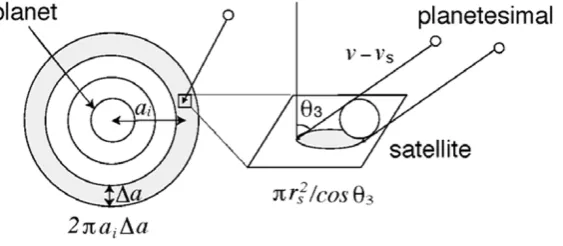
Fig. 1. Schematic illustration of oblique penetration of a planetesimal through anith planetocentric annulus with radiusai and widtha. Hereθ3 is the angle between relative-velocity vector of the planetesimal to the satellite and normal direction of the satellite’s orbital plane, andrsis radius of the satellite.
orbital angular momentum of a grazing satellite 3rp 1/2
[=(G MpRp)1/2/(RH2K)] is given by
Jp(e,i)=
z
(3rp)1/2
= 1 Pp
3
2|b|σd(b)
z(e,i,b, τ, ω)
3rp
·pcol,p(e,i,b, τ, ω)
dτdω
(2π)2db. (8)
In the abovezis thez-component of the specific
planetocen-tric angular momentum given by a colliding planetesimal:
z(e,i,b, τ, ω)=rϕ˙+r2, (9)
where we use a planetocentric cylindrical coordinate for con-venient sake; the position and the velocity of the planetesimal at the collision are given by(r, ϕ,z)and(r,˙ ϕ,˙ ˙z), respec-tively.
2.2 Evaluation of the accretion rate of mass and specific angular momentum supplied to the satellite For a satellite at planetocentric distanceas, the collision
ratePs(e,i,as,rs)and the mean specific planetocentric
angu-lar momentumJs(e,i,as)normalized by the satellite orbital
angular momentumo [=(3as)1/2] are, respectively, given
by
Ps(e,i,as,rs)=
3
2|b|σd(b)pcol,s(e,i,b, τ, ω,as,rs, ϕs)
·dϕsdτdω
(2π)3 db, (10)
Js(e,i,as)=
z
o
= 1 Ps
3
2|b|σd(b) z
o(
e,i,b, τ, ω)
·pcol,s(e,i,b, τ, ω,as,rs, ϕs) ·dϕsdτdω
(2π)3 db, (11)
where pcol,sis unity for collision orbits to the satellite and
zero otherwise. It should be noted that ifJs>1, the specific
angular momentum of the satellite increases and its orbit expands.
Since we neglect satellite gravity, the orbits of planetesi-mals are not affected by the position of the satellite, so that
only one orbital calculation is needed for each planetesimal of given orbital elements. Further we safely expect the prin-ciple of equal a prioriprobabilities in the orbital phase of the satellite. Then, instead of counting direct collisions to each satellite, we merely count number of penetrating orbits through concentric annuli with the center at the planet and widtha(see Fig. 1). When a planetesimal with given or-bital elements penetrates theith annulus, the collision prob-ability between the satellite therein and the planetesimal is given by the ratio of the projection area of the satellite body to the total area of the annulus:
pcol,3D(e,i,b, τ, ω,ai,rs)
= 1
2πaia
·
ai+a/2
ai−a/2 2π
0
pcol,s(e,i,b, τ, ω,as,rs, ϕs)asdϕsdas
= ⎧ ⎨ ⎩
g3rs2
2aia (for penetrating orbits),
0 (otherwise),
(12)
whereaiis the mean radius of theith annulus. In the above,
g3 denotes the enlargement factor for oblique penetration
given by
g3min
1 cosθ3
,3ai
rs
. (13)
Here θ3 is the angle between the incident direction of the
planetesimal in the comoving system for the satellite and normal direction of the orbital plane of the satellite given by
tanθ3=
(rϕ˙−rωs)2+ ˙r2+ ˙z2 ˙
z
, (14)
whereωsdenotes the angular velocity of the satellite given
by
ωs=
G Mp
A3
s
1/2
−1
K =
3 a3
s
1/2
. (15)
The upper limit ofg3in Eq. (13) is derived in Appendix A.
Wefind that 1/cosθ3scarcely exceeds the upper limit 3ai/rs,
wheni >∼0.01, so thatg3is almost independent ofrs. Thus
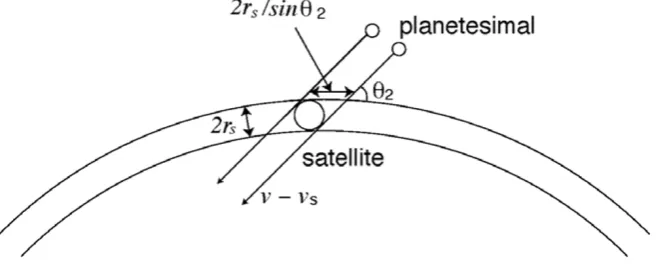
Fig. 2. Same as Fig. 1 but for the two-dimensional case (i =0). Hereθ2is the angle between relative-velocity vector of the planetesimal to the satellite and direction of the satellite’s orbital motion.
for any other radius by multiplying the square of the ratio of the radius to the standard value except extremely lowicases. Wefind that the results have little dependence onaifa is smaller than 0.01. So wefixa=0.01 in the following. In order to know the behavior of Ps in the cases of low
inclination case, we also calculatePsandJsfor purely
two-dimensional cases. When a planetesimal orbit crosses the satellite orbit, the collision probability is given by the ratio of the satellite diameter to the length of the orbital circum-ference (see Fig. 2):
pcol,2D(e,i =0,b, τ,as,rs)
= 2π
0
pcol,s(e,i=0,b, τ,as,rs, ϕs)
dϕs
2π
= g
2rs
πas (for crossing orbits),
0 (otherwise). (16)
Hereg2is the enlargement factor for oblique crossing given
by
g2=min
1 sinθ2
,4
as
2rs
, (17)
whereθ2is the angle between the relative-velocity vector of
the planetesimal to the satellite and the velocity vector of the satellite given by
cosθ2=
asϕ˙−asωs
(asϕ˙−asωs)2+ ˙r2
. (18)
The upper limit ofg2in Eq. (17) can be derived, considering
a parabolic tangential orbit with the satellite orbit. Wefind that orbits with 1/sinθ2 >4
√
as/2rsare very rare, so that
g2is almost independent ofrs.
In order to obtain Ps and Js, we numerically integrate
Eq. (2) using a fourth-order time-step variable Runge-Kutta method. An orbital integration of a planetesimal with given orbital elements is continued until the planetesimal collides with the planet or goes far away from the planet-satellite system.
According to OI98, we modeled spatial distributions of planetesimals as follows. For an uniform case, nondimen-sional surface number densityσd(b)is unity for allb. On the
other hand, for nonuniform cases, planetesimals only exist in
the range ofE ≤ Emax, whereEdenotes the Jacobi integral
given by (e.g., Nakazawa and Ida, 1988)
E =1 2(e
2+
i2)−3 8b
2+9
2,
andEmaxdenotes the maximum value ofE. Thusσd(b)for
nonuniform cases is given by
σd(b)=
0 for|b|<4(e2+i2)/3+12−8Emax/3 1/2
, 1 for|b| ≥4(e2+i2)/3+12−8E
max/3 1/2
. (19) We perform calculations for the uniform case (OI98 calls it the case of Emax = ∞) and two nonuniform cases with
Emax=1.5 and 2.0. In the case ofEmax∼1.5, thefinal spin
angular momentum of the planet was found to be as large as the present total angular momentum of the Earth-Moon system (OI98). We assume that planetesimals are distributed uniformly in the phase space(τ, ω)for all the cases.
3.
Results
3.1 Collision rate of planetesimals to the satellite
Using the methods described in Subsection 2.2, we nu-merically calculate the collision rate of planetesimals to the satellite from the data of more than 104 orbits penetrating each annulus of Fig. 1. Though we only show the results for the case ofrs=0.001, which corresponds toμs=0.01 with
ρp=ρs, one can easily obtainPsfor an arbitrary radius by
multiplying the ratio of geometrical cross sections.
Using Eq. (10) wefirst examine the collision rate of the satellite in a planetesimal disk with uniform spatial distri-bution. Figure 3 shows Ps as a function of as for various
values ofewithfixing the ratioi/eto be 0.5. Wefind the following properties: (1) in all cases Ps decrease with the
increase of as ande, and the simple approximate relation
Ps∝a−s1is valid for 1≤e≤8; (2)Ps(e=i=0)is almost
independent ofasfor as <∼ 0.05 and is approximated as a
power law Ps(e=i = 0)∝ a−s1 for largeras, and similar
as-dependencies ofPscan be seen fore<∼1.0.
Property (1) is explained by using a semi-analytical form of collision rate Ps,2B, which is practically valid fore,i >∼
Fig. 3. Collision rate versus planetocentric distance of the satellite (μs=0.01) in the case of uniform spatial distribution of planetesimals with variouse(0≤ e ≤8) withfixingi/e = 0.5. The solid curves denote numerical solutions and the dashed curves in the case ofe≥1.0 denote analytic solutions given by Eq. (20).
Ps,2B(e,i,as,rs)=
2 π
2
[E(k)K(k)]1/2πrs2
·
1+ 6 asvr2,p
vr,p
2i , (20)
wherevr,pis the random velocity of planetesimals given by
vr,p=
e2+i2 E(k)
K(k)
1/2
. (21)
In the aboveK(k)andE(k)are the complete elliptic integral of thefirst and second kind, respectively, with
k=
3e2
4(e2+i2). (22)
Considering the case that the gravitational energy of the planet 3/as is much larger than the kinetic energy of the
planetesimalv2
r,p/2, we obtain Ps ∝ as−1. On the contrary,
for largereandas,Psbecomes independent ofas.
Compar-ing Ps,2Bwith Ps, wefind Ps coincides well with Ps,2B for √
e2+i2> ∼4.0.
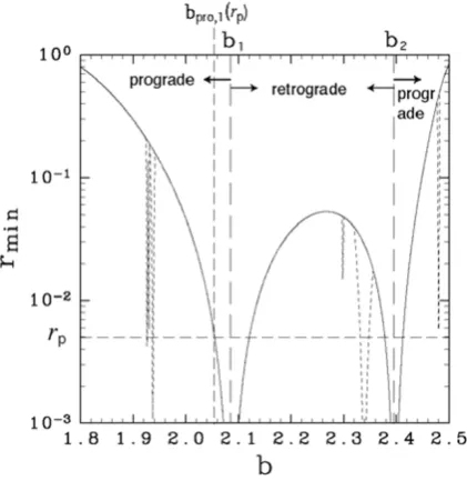
Property (2) can be interpreted from properties of retro-grade orbits of planetesimals around the planet. In the case of e=i =0, wefind that there are no retrograde orbits around the planet (i.e., orbits withϕ <˙ 0 at the time of collisions) withrmin >∼0.06, wherermindenotes the minimum distance
between a planetesimal and the planet, so thatas-dependency
of Ps(e=i =0)changes nearas ∼0.06; the detail is
ex-plained in Appendix B using theb-dependency ofrmin. In
the cases of smalle(<∼1.0), we alsofind that each kink of Ps(e,i)corresponds to the maximumrmin of all retrograde
orbits.
Next, we examine the collision rate of the satellite in plan-etesimal disks with nonuniform spatial distributions. With the decrease of Emax, both Ps and Pp decrease because of
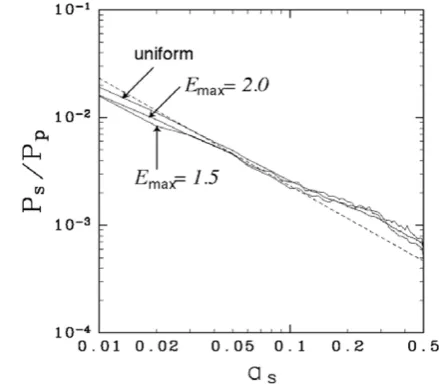
Fig. 4. Ratio of collision rate of the satellite (μs=0.01) to that of the planet for two spatially nonuniform cases (Emax=1.5 and 2.0) and a uniform case withfixing all the cases as(e,i)=(2,1). The dashed curve denotes analytic solutionPs/Pp=rs2/(rpas)(see Eq. (23)).
broadening of the gap of planetesimals in the vicinity of the planet. For example, the values of Ps(e=2,i =1,as)with
Emax = 1.5 are reduced by a factor of about 20 from the
values of Ps(e=2,i =1,as)for the uniform case. Hence,
Eq. (20) is no longer valid for the nonuniform disk. We are rather interested in the ratioPs/Ppthan each absolute value,
since the ratio determines the evolution ofμs. Figure 4 shows
Ps/Pp as a function ofas for Emax = 1.5 and 2.0, and the
uniform case withfixing all the cases as(e,i)=(2.0,1.0); wefind that Ps/Pp is almost independent of Emax. In fact,
Ps/Ppis well approximated by
Ps
Pp
2B =
rs
rp 2 (E
max−9)/2+3/as
(Emax−9)/2+3/rp
, (23)
for √e2+i2 >
∼ 2.0. Since the kinetic energy of random motion of planetesimals, (Emax −9)/2, can be negligible
compared with the planetary potential energy 3/asin the case
of √e2+i2 <
∼ 4.0, Ps/Pp is almost independent of Emax.
In this case, Eq. (23) is simply described as (Ps/Pp)2B =
r2
s/(rpas), which is also shown as a dotted line in Fig. 4. 3.2 Specific angular momentum of planetesimals
sup-plied to the satellite
We here show the angular momentum supplied by plan-etesimals to the satellite. Neglecting planetary growth and tidal torque, we can say thatasdecreases with satellite growth
when the specific angular momentum of the planetesimalsJs
is smaller than unity. For the sake of comparison withJs, we
also calculate mean specific angular momentum supplied to afictitious circumplanetary disk with radiusasafter Herbert
et al.(1986), which is given by
J0(e,i,as)
=
3 2|b|σd(b)
z
o
(e,i,b, τ, ω)pcol,d(e,i,b, τ, ω,as)
dτdω (2π)2db
3
2|b|σd(b)pcol,d(e,i,b, τ, ω,as)
dτdω (2π)2db
,
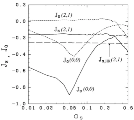
Fig. 5. Specific angular momentums supplied to the satelliteJs(e,i)and to a planetocentric diskJ0(e,i)as functions of planetocentric distance
asfor the case of uniform spatial distribution of planetesimals. Analytic solutionJs,HKgiven by Eq. (25) in the case of(e,i) =(2,1)is also shown.
wherepcol,dis unity for crossing (i =0) or penetrating (i=
0) orbits and zero otherwise. It should be noted that putting g3=1 (org2=1) in Eq. (12) (or in Eq. (16)) Eq. (11) reduces
to Eq. (24). This means that the effect of the orbital motion of the satellite is not included in the value ofJ0whereas it is
taken into account in the value ofJs.
Wefirst calculate Js andJ0for many pairs of(e,i)for a
planetesimal disk with uniform spatial distribution. Figure 5 shows JsandJ0as functions ofasfor the cases of(e,i)=
(0,0)and(e,i)=(2,1), respectively. For(e,i)=(0,0), bothJ0andJsare negative for allas, which means that there
exist more retrograde planetesimals than prograde ones. Be-haviors ofJsandJ0are similar and both have the minimum
values nearas∼0.06. For largeras,JsandJ0increase with
as. This is because number of collisional planetesimals with
prograde orbits around the planet increases withas, whereas
number of retrograde orbits is kept constant. In Appendix B, we explain the detailed behavior of Js(e = i = 0)from
rmin(b)like that ofPs(e=i =0).
For (e,i) = (2,1), both Js and J0 are constant when
as <∼ 0.30, whereas they decrease with increasingas for
largeras. In such higher random-velocity cases incident of
planetesimals is almost isotropic in the frame of reference of the planet, so thatJ0is almost 0. However,Jsis negative even
in these cases, since in the frame of reference of the satel-lite, incident of planetesimals is not isotropic due to orbital motion of the satellite; considering the relative azimuthal velocity of colliding planetesimals (vrϕ= |rϕ˙−rωs|), a
ret-rograde planetesimal withϕ˙ (<0) has largervrϕ than that
of prograde one with same| ˙ϕ|, so that the enlargement fac-tor (g3in Eq. (13)) of collision probability for a retrograde
planetesimal (it has negative z) is larger than that for the
prograde counterpart (see Eq. (14)).
When incident of planetesimals is isotropic in the frame of reference of the planet, Js is analytically obtained from
Eqs. (9) and (12) of HK75:
Fig. 6. Specific angular momentum supplied to the satelliteJs(e,i)for the case of nonuniform spatial distribution (Emax = 1.5 and 2.0) of planetesimals with(e,i) = (2,1). For comparison, the uniform case with the same(e,i)is also shown.
Js,HK= −
1 3
1+ 27 5asvr2,p
1+ 7 asvr2,p
−1
, (25)
which is also shown as a long-dashed curve in Fig. 5. Wefind that Js,HKis almost independent ofasandvrand has a little
deviation from the numerical results of Js. The deviation
becomes smaller for largereif we focus on smallas(<∼0.1).
It should be noted that Jp(e,i) given in Eq. (8) and
J0(e,i,as) are the same quantity for the two-dimensional
case. The previous studies showed that Jpis about−0.1 for
e = i = 0 (Ida and Nakazawa, 1990; Lissauer and Kary, 1991; Dones and Tremaine, 1993a; OI98), which well coin-cides with the value ofJ0withas∼0.01. We alsofind that
J0 is almost zero fore >∼2.0, which is consistent with the
previous studies ofJp.
Next, we show the results of Js for nonuniform disks.
Figure 6 shows Js as a function ofas for two nonuniform
cases withEmax=1.5 and 2.0, and an uniform case. All of
the cases, wefix(e,i)=(2,1). In the nonuniform cases,Js
becomes positive for smallEmax, which means that there exist
more prograde planetesimals than retrograde ones. Hence, in this case, accretion of planetesimals boosts up the angular momentum of the planet-satellite system. However,Jsnever
exceeds unity, so thatasinevitably decreases with satellite
growth. These results for smallEmaxare consistent with the
case of planetary spin; the accretion of planetesimals with smallEmaxaccounts for the rapid prograde spin of the planet,
but the outcoming spin rate is much smaller than the value required for rotational instability (OI98).
3.3 Evolution of planet-satellite systems
The evolution of the mass ratioμscan be expressed by
whereτgrow,pis the growth time of the planet given by
τgrow,p=
Heredis the surface density of planetesimals.
The evolution of the semimajor axisascan be expressed
symbolically by
drag, tidal repulsion, and gas drag, respectively. To simplify the problem we here neglect the effect of gas drag (which will be discussed in Subsection 5.3). The effect of accretion drag is given by
wherefirst and second terms originate from accretion of plan-etesimals to the satellite and to the planet, respectively.
The satellite affects the repulsive force from the planet by tidal interaction whenasis larger than the so-called
synchro-nized radiusrsyn =(3/ω2p)
1/3, whereω
p is the normalized
spin angular velocity of the planet. The effect of tidal repul-sion is given by (e.g., Mignard, 1979)
1
wherek2 andQp are, respectively, the Love number of the
second degree and the quality factor of the planet. Herek2for
a homogeneous and incompressible planet can be estimated by (Love, 1934)
REandk2Eare the radius and the Love number of the present
Earth, respectively, andmp =Mp/ME. The ratio of the two
time scalesτacc/τtidalis given by
τacc
where f˜denotes the tidal parameter defined by
˜
tidal repulsion becomes dominant in comparison with accretion drag. Taking the present values of parameters k2E = 0.3 and Qp = 10, and the standard valueτ˜grow,E =
Fig. 7. Evolution of orbital radiusasand mass ratioμsof the satellite in the
as–μsplane in the swarm of planetesimals with(e,i)=(2,1). (a) Tidal parameter f =0.21, which corresponds to a spatially uniform disk. (b)
f =3.9, which corresponds to a nonuniform disk withEmax=1.5. Each vector component is proportional to inverse of corresponding evolutional time scale (but truncated by an upper limit). The solid curves show the stationary mass ratio wheredμs/dt =0. The dashed curves show the balanced semimajor axis wheredas/dt=0. The satellitefinally evolves into the equilibrium points wheredμs/dt=das/dt=0.
where 0 is the surface density of planetesimals for the
minimum-mass solar nebula model at 1 AU (Hayashiet al., 1985).
Here we assume that the planet spins so rapidly that exert-ing enough tidal repulsion. Figure 7 shows change rates ofas
andρp = ρs. Further, we choose two types of spatial
dis-tributions of planetesimals, a uniform one (Fig. 7(a)) and a nonuniform one (Fig. 7(b)). The spatial distribution of plan-etesimals affects the normalized tidal parameter f through Pp; wefind that Fig. 7(a) corresponds to the case off =0.21
and Fig. 7(b) to f = 3.9. The solid curves show the sta-tionary mass ratio where dμs/dt = 0. If μs is smaller
than the stationary mass ratio,μsincreases with growth,
be-cause smaller satellites have larger cross sections per mass. The dashed curves show the balanced semimajor axis where das/dt =0 (in other words,τacc/τtidal =1). The balanced
semimajor axis for the nonuniform case is larger than that for the uniform case, because of the effects of larger f (which comes from smallerPp) and larger Js(see Fig. 6). Since the
evolution time scale ofasis generally much shorter than that
ofμs,asevolves toward the balanced semimajor axis quickly.
Then, with keepingasto be the balanced semimajor axis,μs
evolves toward the stationary mass ratio. We denote thefinal locus the equilibrium point, wheredas/dt =dμs/dt =0,
and its mass ratioμs,eq.
Note thatμs,eqis the maximum mass ratio of the satellite if
the satellite grows from a smaller embryo. Wefind thatμs,eq
for the nonuniform case is smaller than that for the uniform case and both are smaller thanμM. However, one should note
that we show here the case with(e,i)=(2,1)as a nominal example. In Section 4 we consider more realistic(e,i)and examine whetherμs,eqexceedsμM.
In the case of a smaller planetary mass (mp < 1.0), the
balanced radius becomes smaller (see Eq. (32)) and μs,eq
becomes larger in comparison with the case ofmp = 1.0.
Also, the value of f would not be a constant during the ac-cretion. Thus,μs,eqchanges with growth, so that the final
mass ratioμs will deviate fromμs,eq. Let us simply
esti-mate how much thefinalμswould deviate fromμs,eq, using
Eq. (26). For the case thatμsμs,eq, the time scale of the
mass-ratio evolution (i.e., μs(dμs/dt)−1)is much shorter
thanτgrow,p. Equatingμs(dμs/dt)−1withτgrow,pin Eq. (26),
wefind that within the time ofτgrow,p,μs will be converge
μs,eqwithin a factor 2 in spite of the initial value ofμs. Thus,
we can roughly estimate thefinal mass ratios of long-lasting co-accretion cases from the mass ratio of the equilibrium pointμs,eq(see Subsection 4.1).
On the other hand, ifmpbecomes unity and stop growing
beforeμsgetting closer toμs,eq, the value ofμsat this point
should be frozen as thefinal value. Thus, when discussing the co-accretion after late-stage formation of the satellite (such as the giant-impact hypothesis), we should directly deal with time evolution ofμsandasinstead of using onlyμs,eq(see
Subsection 4.2).
4.
Two Types of Co-Accretion Scenarios for Lunar
Origin
In Subsection 3.3 we assumed that the planet spins so rapidly that tidal repulsion prevents the satellite from spi-raling into the planet. We here demonstrate two types of promising situations which satisfy the rapid-spin condition and would bring forth the present Earth-Moon system. One is a long-lasting co-accretion case, in which an initial satellite embryo much smaller than the present Moon successively grew in a swarm of low-Jacobi-energy planetesimals in the
solar nebula, and the other is an additional co-accretion case, in which a satellite as large as the present Moon was formed by a giant impact in the later stage, but not in thefinal stage, of Earth formation.
In both cases, the large angular momentum of the Earth-Moon systemLEMas well as the large relative mass of the
MoonμMcan be accounted for within possible ranges of
ini-tial masses and angular momentum. These ranges of iniini-tial values are important for us to constrain the conditions of pos-sible Moon-forming events from the dynamical viewpoint.
It should be noted that if the Moon gained most of the mass during co-accretion, it might be hard to explain the bulk composition of the Moon, which is different from that of the Earth (e.g., Wood, 1986). It is a severe obstacle es-pecially for a long-lasting co-accretion case. But it is not clear from the geochemical constraints how much the mass is allowed to accumulate onto the Moon during co-accretion. In order to overcome the geochemical constraints, one must first clarify a picture of accretional and dynamical evolution of co-accretion. So we here confine our discussion only to the dynamical constraints.
4.1 Co-accretion from small embryos
In this scenario, we consider that large spin angular mo-mentum of the planet was supplied by a swarm of low-Jacobi-energy planetesimals with nonuniform spatial distribution. OI98 showed that the final planetary spin rate by accre-tion of planetesimals with nonuniform spatial distribuaccre-tion of Emax<∼1.5 is large enough to explain 1LEM, whereEmaxis
the maximum Jacobi integral of planetesimals (see Eq. (19)). Such lower values of the maximum Jacobi integral as well as lower random velocities is expected when the spatial and velocity distributions of the planetesimals are determined mainly by the balance between gravitational scattering by the planet and gas drag by the solar nebula.
We examine the case that a small satellite embryo evolves under the swarm of planetesimals with smallEmax. In
Sub-section 3.3, we found that the relative mass of the satel-lite evolves toward the equilibrium mass ratio μs,eq.
In-serting the relationdμs/dt = das/dt = 0 into Eqs. (26)
and (28) and using the relation Ps/Pp = rs2α/(rpas)(see
Eq. (23)) (here we multiply the focusing factor of the satel-liteα=1+(vesc,s/vr,s)2, which is not negligible for a
lunar-sized satellite), we can estimate the equilibrium mass ratio as
μs,eq=
2(1−Js)+4/3
3√3f m˜ prp5
6/19
ρs
ρp
−26/19
rpα 39/19
=3.3×10⁻³f−6/19m−p6/19, (35)
where we adopt appropriate values of parameters: Js=0.25
(the averaged value for the case of(e,i)=(2,1)andEmax=
1.5; see Fig. 6),rp =0.004,ρs/ρp=0.6 (the present values
for the Earth-Moon system), andα = 1.2 (for the case of μs,eq =μM). Eq. (35) suggests that with decreasing f, the
larger satellite is produced under the benefit of gravitational focusing by the planet, since the semimajor axis of the satel-lite is kept smaller. Choosingmp = 1.0 and f =3.9, we
find thatμs,eqis about one tenth ofμM(see Fig. 7b). Since
f depends on the uncertain values of the parametersPp,d,
proba-ble minimum value of f at the later stage of Earth formation (mp∼1.0) in order to check the possibility thatμs,eqreaches
μM.
Wefirst evaluate maximum value of the collision ratePp,
which is a function of mean eccentricitye, inclinationi, and maximum Jacobi integralEmaxof planetesimals. In the later
stage of planetary accretion, small fragments produced by mutual collisions of planetesimals are expected to make a main contribution to the planetary growth in the solar nebula (Wetherill and Stewart, 1993). The eccentricities and incli-nations of these small fragments are estimated ase∼3 and i e under the balance between gravitational scattering by the proto-Earth and gas drag of the solar nebula (OI98). The condition that thefinal angular momentum of the Earth-Moon system reaches 1LEMrestricts Emax must be smaller
than 1.5. Under these values ofe,i,andEmax, we obtain the
maximum value ofPpto be about 0.01 (OI98). It should be
noted that such a large value of Ppcan be acheived by the
effect of smalliprevailing against that of smallEmax.
The maximum value of surface densitydof solid material
in the circumsolar disk can be somewhat larger than that of the minimum-mass model0(Hayashiet al., 1985), whereas
in the later stage of Earth formation it would decrease from the initial value. So we choose0to be the maximum value
of the surface density at the later stage of Earth formation. We next estimate the maximum value of plausibleQp. The
value for the present Earth isQp ∼12 (e.g., Lambeck, 1980;
Burns, 1986); the main contribution is due to oceanic tides. Whereas Qp would be 370 if solid tides only (Ray et al.,
1996). The value ofQpfor a planet with the surface ocean is
expected to increase with the depth of the ocean (Goldreich and Soter, 1966; Sagan and Dermott, 1982). In the course of planetary accretion we must consider the effect of the surface magma ocean, which would be formed when the mass of the proto-Earth exceeds 0.1ME (e.g., Kaula, 1979; Sasaki and
Nakazawa, 1986). At the later stage of the Earth formation, the magma ocean would be deep and fully melted due to the strong green-house effect of the protoatmosphere (Abe and Matsui, 1985, 1986; Sasaki and Nakazawa, 1990) and the large values of estimated Pp(i.e.,τ˜grow,E <∼106 years).
Hence, we expect that contribution of the magma ocean to tidal dissipation of the proto-Earth is rather small, so that we here adopt the maximum value ofQpto be 400.
It should be noted that the maximum values of the parame-ters given above were consistently realized if the Earth grew rapidly. Re-normalizing each parameter by the correspond-ing maximum value, we can rewrite Eq. (34) as
f =0.015
Qp
400
−1 d
0 −1
Pp
1×10⁻² −1
. (36)
Figure 8 shows the equilibrium points on theμsvs.asplane
for f = 0.015 and 1.0 with mp = 1.0, Js = 0.25, and
ρs/ρp = 0.6. Note thatμs,eq exceeds μM in the case of
f = 0.015. In fact, μs,eq ∼ μM when f ∼ 0.03 (see
Eq. (35)).
This means that, as long as from the dynamical viewpoint, the Moon could be grown up from a small embryo, if the following conditions were satisfied for the long-lasting co-accretion:
Fig. 8. Tidal-parameter(f)dependency of the mass ratio at the equilibrium pointμs,eqin theas–μsplane. In the case of the minimum value of f (=0.015, see Eq. (37)),μs,eqhas the maximum value.
(1) The Earth and the Moon grew up in the solar nebula, so that the growth time of the Earth is short enough (τ˜grow,E <∼106years) and that large angular momentum
was supplied by planetesimals with smallEmax.
(2) Owing to fully-melted and deep magma ocean through accretion,Qpof the proto-Earth was kept large (∼400).
(3) The satellite avoided from spiraling into the planet owing to gas drag by the solar nebula (see Subsection 5.3).
These are rather strong dynamical constraints, so that we should examine whether these constraints are really satisfied in the course of Earth accretion. In the future work we will be able to clarify the possibility of realization of the long-lasting co-accretion from these dynamical constraints, besides from the frequentry-discussed geochemical constraints.
Until now, we focused on thefinal mass ratio of the lite. Here, we estimate the minimum mass of an initial satel-lite embryo from which the Moon could grow up succes-sively. As shown in Section 3, the embryo with small mass ratio grows around the balanced radius, which increases with the mass ratio. We can estimate the minimum mass by equat-ing the balanced radius with the Roche radiusrR∼2.5rp∼
0.01, within which planetary tides prevent the embryo from growing. Note that the synchronized radius is expected to be smaller thanrR, since planetary rotation is rapid enough due
to accumlation of planetesimals with small Emax (∼ 1.5).
The minimum mass Ms,min of the initial embryo is given
approximately from Eqs. (23), (29), and (30) as
Ms,min =6.3×10⁻³MM
f 0.015
−3/4
·mp
0.1
1/4 rR
2.5rp 33/8
. (37)
Note that dependency of Ms,min on mp is rather small, so
smaller than ours. This is because their adopted random velocity of planetesimals was larger (i.e., smaller Pp) and
Qpwas smaller than ours.
4.2 Co-accretion after the Moon-forming giant impact
Recently, the Moon-forming giant impact is considered to have occurred during Earth accretion (Cameron and Canup, 1998a, b; Canupet al., 2001). In this scenario, the large spin angular momentum as well as a lunar-sized satellite were produced by the giant impact itself. Then, the mass ratio and the angular momentum of the Earth-Moon system would be changed through co-accretion thereafter. After the dissipa-tion of the solar nebular, random velocities of planetesimals were determined by the balance between gravitational scat-tering by the planet and dissipation due to mutual inelastic collisions. The balanced values of the random velocities become larger than those in gaseous environment, so that net angular momentum brought by planetesimals was almost zero and the planet would spin down in the post giant-impact stage.
In order to confine dynamical parameters (e.g., mass ratio, angular momentum) immediately after the giant impact, we go back evolution of the Earth-Moon system from thefinal stage of Earth formation to the past. The changes ofμsand
ascan be expressed by Eqs. (26) and (28), respectively, and
the change ofωpby
1 ωp
dωp
dt = − 5 3
1 τgrow,p −
1 2
μs √
3as
I r2 pωp
1 τtidal,
(38)
where I is the normalized moment of inertia of the planet (we here adopt I =0.33, the value for the present Earth). In Eq. (38), thefirst term of the right-hand side denotes the effect of planetesimal accretion and the second term the effect of tidal interaction with the satellite. We also calculate the total angular momentum of the planet-satellite system,Lps=
I MpRp2ωpK+Ms
G MpAs. We choose the starting values
of the mass ratio to beμM, the total angular momentum to
beLEM, andasto be the balanced radiusas,baforμs=μM
(see Subsection 3.3).
We halt each backward integration if one of the following conditions is satisfied:
(1)as>as,ba,
(2)as<rR,
(3)ωp>5600.
Condition (3) corresponds to the marginal value of the sec-ular bar instability of a rapidly rotating planet (Durisen and Gingold, 1986). During the integration we keep the semi-major axis of the satellite to be the balanced radius at each time; otherwise the integration would halt more rapidly.
We determine the parameters for the integration, i.e., the mean random velocity, the surface density of planetesimals, and the specific angular momentums supplied to the planet and the satellite, as follows.
The mean random velocity vr of planetesimals in
gas-free environment is given by the balance between gravita-tional scattering by the planet and dissipation due to mu-tual inelastic collisions. The time scale of increasing ofvr
by planet’s gravitational scattering (i.e., the viscous stirring
time) is given by (Ida, 1990; Ida and Makino, 1993)
Tvs=
ce1
nprp2
v
r
vesc,p 4
, (39)
wherece1is a numerical factor (∼0.10),np is the effective
surface number density of protoplanets (one of which is the proto-Earth), andvesc,p(∼35)is the escape velocity of the
planet. On the other hand, the time scale of mutual collisions of planetesimals is given by (Greenzweig and Lissauer, 1990; Ohtsuki, 1993)
Tcol=
ce2
ndr2
, (40)
wherece2 is a numerical factor (∼ 0.54),nd is the surface
number density of planetesimals, andr is the sum of plan-etesimal radii. Here we assumed thate=2iand that masses of all the planetesimals are equal. EquatingTvswithTcol, we
obtain
vr =0.4
npMp/d
2.0
1/4m/M p
10−6 1/12
vesc,p, (41)
where m is the mass of planetesimals. According to the above equation, we here choose the value of eccentricity and inclination of planetesimals as(e,i)=(15,7.5).
We assume that the surface density of planetesimals is kept constant with the value of the minimum-mass model during the growth for simplicity. Then in gas-free environ-ment, the growth time of the Earth given by Eq. (27) is about 6.0×10⁷ years, which is two orders of magnitude longer
than that for accretion in the gaseous environment adopted in Subsection 4.1.
Because of the large random velocities of planetesimals, we adopt that specific angular momentums supplied to the planet and to the satellite are, respectively, Jp=0 andJs= −0.2 (see Subsection 3.2), which are fairly smaller than those in the gaseous environment (Jp∼0.2,Js∼0.1).
Using these parameters, we perform the integration. Fig-ure 9 shows the results; changes of ps (= Lps/LEM),ωp,
as, andμs as functions of mp for two different values of
f =60 (long-dashed curves) and 1.5 (solid curves), which correspond to the cases ofQp=10 and 400, respectively. In
both cases the backward integrations were halted by satisfy-ing Condition (3) (see Fig. 9(b)) whenmp ∼0.55, because
a smaller planet cannot have angular momentum as large as that of the Earth-Moon system. Hence, the giant impact should occur after the mass of the proto-Earth exceeds about half of the present mass.
Figure 9(a) shows thatpsdecreases with increasingmp.
This is because of collisional-planetesimals anisotropy due to the orbital motion of the satellite (see Subsection 3.2). We find that the angular momentum supplied by the giant impact should be a factor 0.5|Js|(1−mp)(formp∼0.5, about 5%)
larger than 1LEM. The giant-impact simulations by Cameron
and Canup (1998a) in the case ofmp =0.6 (where we use
mp as the total mass of the impactor and the target) show
that mass of the disk generated by an impact with the total angular momentum 1.2LEM is twice as large as that with
1.0LEM. Thus, even 5% increase of total angular momentum
Fig. 9. Evolutions of total angular momentumps(a), planet’s spin angular velocityωp(b), satellite’s planetocentric distanceas(c), and relative mass μs(d) as functions of planet mass for two perfect accretion cases with f =1.5 (solid curves) and 60 (long-dashed curves), and one non accretion case (d Ms/dt=0)with f =60 (short-dashed curves). The integrations start frommp=1.0 to the past. The starting values forμsandpsare the present values of the Earth-Moon system (μs=μM,ps=1.0), butasis determined from a given value of f (as=as,ba) andωpis determined from all these values. In all the cases, the backward integrations are halted where rotational instability of the planet will occur (ωp>5600).
protoMoon if co-accretion after the giant impact is taken into account.
Figure 9(d) shows thatμsincreases withmp. This is
be-cause the Moon has larger collision cross section per mass than that of the Earth. In other words,μs,eqfor the case of
largervr(as adopted in Fig. 9) exceedsμMeven for the case
of larger f. The value ofμsincreases more rapidly with
de-creasing f because a satellite with smaller balanced radius (see Fig. 9(c)) receives a larger benefit of planetary focus-ing. In any cases, however, mass-ratio changes are rather small compared with the situation in Subsection 4.1 because of smaller mass change of the Earth itself.
Until now, we assumed that the coalescence probability between the satellite and planetesimals to be unity. But in high-speed collisions, the total mass of escaping ejecta from the satellite might become comparable to the mass of a im-pactor (for a full discussion of ejecta, see Subsection 5.2). Here we also calculate the post-giant-impact co-accretion
in an extreme case that d Ms/dt = 0. We assume that all
of escaping ejecta from the satellite also escape from the planetary Hill sphere and that their mean specific geocen-tric angular momentum is same as that of the satellite. We perform integration of the co-accretion evolution backward frommp =1.0 for the case of f =60. The results are also
shown in Fig. 9 (short-dashed curves). Figure 9(a) shows that ps decreases with increasingmpmuch faster than the
perfect accretion cases, since escaping ejecta take away large amount of angular momentum from the planet-satellite sys-tem. With a increase in total mass of escaping ejecta from the satellite, largerpsis allowed immediately after the giant
impact.
5.
Discussion
5.1 Comparison with results of giant-impact simula-tions
Fig. 10. Mass ratio of a impact-generated satellite relative to total colliding mass as a function of impact angular momentum normalized byL∗(dotted curve) withfixing an impactor-to-target mass ratio to be 3:7 and an impact velocity to be the mutual escape velocity. Three evolutional curves, which correspond to the results shown in Fig. 9 (solid, short-dashed, and long-dashed curves), are also shown. The converging point of three curves corresponds to the present state of the Earth-Moon system.
mass ratio and the total angular momentum, we went back the evolution of the Earth-Moon system to the past. Thus, if all the dynamical quantities of the outcome of a giant-impact simulation locate on the evolution curves of the cor-responding quantities obtained in our calculation, the gen-erated system willfinally reach to the present Earth-Moon system through co-accretion. Here we compare our results with the results of the giant-impact simulations.
Canup et al. (2001) compiled the results of the impact simulations, all employing an impactor-to-target mass ratio of 3:7 and equalizing the impact velocity with the mutual escape velocity of the target and the impactor. They showed that mass of the impact-generated satelliteMsis given by
Ms
Mt =
0.15
Limp
L∗
3.83
−0.064
Limp
L∗
3.40
0.5< Limp L∗ <1.0
, (42)
whereLimpand Mt are the impact angular momentum and
the total mass of the impactor and the target, and L∗ = 2.91(Mt/ME)5/3LEMdenotes the planetary angular
momen-tum spinning at the maximum rate for rotational instability. Figure 10 shows the relation betweenMs/MtandLimp/L∗
given by Eq. (42) (dotted curve). It is clear thatMs/Mt
dras-tically increases with Limp/L∗. In the samefigure, we also
re-plot three evolution curves shown in Fig. 9. Note that the converging point of the three curves corresponds to the present state of the Earth-Moon system. An important fea-ture of this figure is that mass of a satellite formed by a impact with the present total mass and the angular momen-tum of the Earth-Moon system is much smaller than that of the Moon. This problem has been discussed by multiple pre-vious works (Canup and Esposito, 1996; Idaet al., 1997; Cameron, 1997, Cameron and Canup, 1998a, b; Canupet
al., 2001). If smaller total mass is considered, larger satel-lite mass is achieved owing to increasing of Limp/L∗. We
find each evolution curve has a point of intersection with the curve represented by Eq. (42). It should be noted that if a gi-ant impact produces a planet-satellite system corresponding to each point of intersection, the generated system evolves into the Earth-Moon system through co-accretion with the corresponding conditions. From Fig. 9(d), we canfind that the value ofmpof at the three points of intersection are
al-most equal to 0.7. This suggests that the Moon-forming impact was occurred when Mt 0.7ME, regardless of the
conditions of subsequent co-accretion stage.
However, Eq. (42) is confined to the case that the impactor-to-target mass ratio to be 3:7 and the impact velocity to be the mutual escape velocity. Giant-impact simulations in wider parameters region are desirable.
5.2 Coalescence probability between the satellite and planetesimals
In most of the calculations, we assumed that coalescence probability between the satellite and planetesimals to be unity. It might fairly decrease in high-speed collisions. Here, we estimate the coalescence probability Pco, i.e.,
Pco=1−
mesc
m (1−qre), (43)
wherem andmesc denote, respectively, the colliding
plan-etesimal mass and the total mass of ejecta escaping from the satellite, andqreis the mass fraction of re-accumulating
ejecta which once escaped from the gravitational sphere of the satellite to the circumplanetary orbit.
Using the scaling laws of impact cratering in the gravity regime given by Housenet al.(1983), we estimate the escap-ing massmescas a power-law function of impact velocity of
the planetesimalvimp=(vr2+9/as+v2esc,s)
1/2. Adopting the
coefficients and the power-law indices determined from labo-ratory experiments of sand targets (Holsapple, 1993; Housen et al., 1983), we obtain
mesc
m =0.12
vimp
vesc,s 1.23
. (44)
Setting as to be the balanced radius, we obtain vimp ∼
2.3vesc,s for μs = μM and vimp ∼ 12.5vesc,s for μs =
Ms,min/(0.1ME) in the gaseous environment discussed in
Subsection 4.1. In the gas-free environment discussed in Subsection 4.2, we havevimp ∼2.6–3.2vesc,s. Putting these
values in Eq. (44), we havemesc/m ∼0.33–2.7 and 0.39–
0.50, respectively. A small initial embryo as evaluated in Eq. (37) ejects mass more than impactor mass, which would prevent the satellite growth (Pco<0), ifqreis small enough.
Hence, the minimum mass of the initial embryo might be larger than that in the perfect accretion case. On the other hand, even forqre = 0, the satellite with the mass ratio as
large as that of the Moon can safely grow (Pco>0) in both
situations in Subsection 4.1 and Subsection 4.2, though the growth rate would be reduced. For the situation in Subsection 4.1, we estimate theμs,eqagain adopting imperfect accretion
given by Eqs. (43) and (44) withqre = 0, andfind that the
conditionμs,eq > μM is still satisfied for f ∼0.015. Note