1
Tutorial on EM Algorithm
Loc Nguyen
Sunflower Soft Company, Vietnam Email: [email protected]
Abstract
Maximum likelihood estimation (MLE) is a popular method for parameter estimation in both applied probability and statistics but MLE cannot solve the problem of incomplete data or hidden data because it is impossible to maximize likelihood function from hidden data. Expectation maximum (EM) algorithm is a powerful mathematical tool for solving this problem if there is a relationship between hidden data and observed data. Such hinting relationship is specified by a mapping from hidden data to observed data or by a joint probability between hidden data and observed data. In other words, the relationship helps us know hidden data by surveying observed data. The essential ideology of EM is to maximize the expectation of likelihood function over observed data based on the hinting relationship instead of maximizing directly the likelihood function of hidden data. Pioneers in EM algorithm proved its convergence. As a result, EM algorithm produces parameter estimators as well as MLE does. This tutorial aims to provide explanations of EM algorithm in order to help researchers comprehend it. Moreover some improvements of EM algorithm are also proposed in the tutorial such as combination of EM and third-order convergence Newton-Raphson process, combination of EM and gradient descent method, and combination of EM and particle swarm optimization (PSO) algorithm.
Keywords: expectation maximization, EM, generalized expectation maximization, GEM, EM convergence.
1. Introduction
Literature of expectation maximization (EM) algorithm in this tutorial is mainly extracted from the preeminent article “Maximum Likelihood from Incomplete Data via the EM Algorithm” by Arthur P. Dempster, Nan M. Laird, and Donald B. Rubin (Dempster, Laird, & Rubin, 1977). For convenience, let DLR be reference to such three authors.
We begin a review of EM algorithm with some basic concepts. Before discussing main subjects, there are some conventions. For example, if there is no additional explanation, random variables are denoted as uppercase letters such as X, Y, and Z. Bold and uppercase letters such as X and R denotes algebraic structures such as spaces and fields. By default, vectors are column vectors. For example, given two vectors X and Y and two matrices A and B:
𝑋 = ( 𝑥1 𝑥2 ⋮ 𝑥𝑟
) 𝑌 = (
𝑦1 𝑦2 ⋮ 𝑦𝑟
)
𝐴 = (
𝑎11 𝑎12 ⋯ 𝑎1𝑛 𝑎21 𝑎22 ⋯ 𝑎2𝑛
⋮ ⋮ ⋱ ⋮
𝑎𝑚1 𝑎𝑚2 ⋯ 𝑎𝑚𝑛
) 𝐵 = (
𝑏11 𝑏12 ⋯ 𝑏1𝑘 𝑏21 𝑏22 ⋯ 𝑏2𝑘
⋮ ⋮ ⋱ ⋮
𝑏𝑛1 𝑏𝑛2 ⋯ 𝑎𝑛𝑘 )
Matrix A is squared if m = n. Matrix Λ is diagonal if it is squared and its elements outside the main diagonal are zero:
2
Λ = (
𝜆1 0 ⋯ 0
0 𝜆2 ⋯ 0
⋮ ⋮ ⋱ ⋮
0 0 ⋯ 𝜆𝑟
)
Let I be identity matrix or unit matrix, as follows:
𝐼 = (
1 0 ⋯ 0
0 1 ⋯ 0
⋮ ⋮ ⋱ ⋮
0 0 ⋯ 1
)
Let superscript “T” denote transposition operation for vector and matrix, as follows:
𝑋𝑇 = (𝑥
1, 𝑥2, … , 𝑥𝑟)
𝐴𝑇 = (
𝑎11 𝑎21 ⋯ 𝑎𝑟1 𝑎12 𝑎22 ⋯ 𝑎𝑟2
⋮ ⋮ ⋱ ⋮
𝑎1𝑝 𝑎2𝑝 ⋯ 𝑎𝑟𝑝 )
Dot product or scalar product of two vectors can be written with transposition operation, as follows:
𝑋𝑇𝑌 = ∑ 𝑥𝑖𝑦𝑖 𝑟
𝑖=1
However, the product XYT results out a matrix as follows:
𝑋𝑌𝑇 = (
𝑥1𝑦1 𝑥1𝑦2 ⋯ 𝑥1𝑦𝑟 𝑥2𝑦1 𝑥2𝑦2 ⋯ 𝑥2𝑦𝑟
⋮ ⋮ ⋱ ⋮
𝑥𝑟𝑦1 𝑥𝑟𝑦2 ⋯ 𝑥𝑟𝑦𝑟 )
The length of module of vector X in Euclidean space is:
|𝑋| = √𝑋𝑇𝑋 = √∑ 𝑥 𝑖2 𝑟
𝑖=1
The product of two matrices is:
𝐴𝐵 = 𝐶 = (
𝑎11 𝑎12 ⋯ 𝑎1𝑘 𝑎21 𝑎22 ⋯ 𝑎2𝑘
⋮ ⋮ ⋱ ⋮
𝑎𝑚1 𝑎𝑚2 ⋯ 𝑎𝑚𝑘 )
𝑐𝑖𝑗 = ∑ 𝑎𝑖𝑣𝑏𝑣𝑗 𝑛
𝑣=1
Matrix A is symmetric if aij = aji for all i and j. If A is symmetric then, AT = A. If both A and B are symmetric then, they are commutative such that AB = BA.
Suppose f(X) is scalar-by-vector function, for example, f: Rr → R where Rr is r-dimensional real vector space. The first-order derivative of f(X) is gradient vector as follows:
𝑓′(𝑋) = ∇𝑓(𝑋) =d𝑓(𝑋)
d𝑋 = 𝐷𝑓(𝑋) = ( 𝜕𝑓(𝑋)
𝜕𝑥1 ,
𝜕𝑓(𝑋) 𝜕𝑥2 , … ,
𝜕𝑓(𝑋) 𝜕𝑥𝑟 )
Where 𝜕𝑓(𝑋)
𝜕𝑥𝑖 is partial derivative of f with regard to xi. So gradient vector is row vector. The
3
𝑓′′(𝑋) = d
2𝑓(𝑋)
d𝑋2 = 𝐷2𝑓(𝑋) =
(
𝜕2𝑓(𝑋) 𝜕𝑥12
𝜕2𝑓(𝑋) 𝜕𝑥1𝜕𝑥2 ⋯
𝜕2𝑓(𝑋) 𝜕𝑥1𝜕𝑥𝑟 𝜕2𝑓(𝑋)
𝜕𝑥2𝜕𝑥1
𝜕2𝑓(𝑋) 𝜕𝑥22 ⋯
𝜕2𝑓(𝑋) 𝜕𝑥2𝜕𝑥𝑟
⋮ ⋮ ⋱ ⋮
𝜕2𝑓(𝑋) 𝜕𝑥𝑟𝜕𝑥1
𝜕2𝑓(𝑋) 𝜕𝑥𝑟𝜕𝑥2 ⋯
𝜕2𝑓(𝑋) 𝜕𝑥𝑟2 )
Hessian matrix is squared matrix. Function f(X) is called nth-order analytic function or nth-order smooth function if there is existence and continuity of kth-order derivatives of f(X) where k = 1, 2,…, n. Function f(X) is called smooth enough function if n is large enough. According to Schwarz’s theorem (Wikipedia, Symmetry of second derivatives, 2018), if f(X) is second-order smooth function then, its Hessian matrix is symmetric.
Now we skim through an introduction of EM algorithm. Suppose there are two samples X
and Y, in which X is hidden space (missing space) whereas Y is observed space. We do not know X but there is a mapping from X to Y so that we can survey X by observing Y. The mapping is many-one function φ: X → Y and we denote X(Y) as all 𝑋 ∈ 𝑿 such that φ(X) = Y. So we have X(Y) = {X: φ(X) = Y}. Let f(X | Θ) be probability density function of random variable 𝑋 ∈ 𝑿 and let g(Y | Θ) be probability density function of random variable 𝑌 ∈ 𝒀. Note, Y is also called observation. Equation 1.1 specifies g(Y | Θ) as integral of f(X | Θ) over X(Y).
𝑔(𝑌|Θ) = ∫ 𝑓(𝑋|Θ)d𝑋
𝑿(𝑌)
(1.1) Where Θ is probabilistic parameter represented as a column vector, Θ= (θ1, θ2,…, θr)T in which each θi is a particular parameter. For example, normal distribution has two particular parameters such as mean μ and variance σ2 and so we have Θ = (μ, σ2)T. Note that, Θ can degrades into a scalar as Θ = θ. The conditional probability density function of X given Y, denoted k(X | Y, Θ), is specified by equation 1.2.
𝑘(𝑋|𝑌, Θ) =𝑓(𝑋|Θ)
𝑔(𝑌|Θ) (1.2)
DLR (Dempster, Laird, & Rubin, 1977, p. 1) considered X as complete data and Y as incomplete data because the mapping φ: X → Y is many-one function. In general, we only know Y, f(X | Θ), and k(X | Y, Θ) and so our purpose is to estimate Θ based on such Y, f(X | Θ), and k(X | Y, Θ). Pioneers in EM algorithm firstly assumed that f(X | Θ) belongs to exponential family with note that many popular distributions such as normal, multinomial, and Poisson belong to exponential family. Although DLR (Dempster, Laird, & Rubin, 1977) proposed a generality of EM algorithm in which f(X | Θ) distributes arbitrarily, we should concern exponential family a little bit. Exponential family (Wikipedia, Exponential family, 2016) refers to a set of probabilistic distributions whose density functions have the same exponential form according to equation 1.3 (Dempster, Laird, & Rubin, 1977, p. 3):
𝑓(𝑋|Θ) = 𝑏(𝑋) exp(Θ𝑇𝜏(𝑋)) 𝑎(Θ)⁄ (1.3)
Where b(X) is a function of X, which is called base measure and τ(X) is a vector function of X, which is sufficient statistic. Equation 1.3 expresses the canonical form of exponential family. Let Ω be the convex set such that Θ ∈ Ω. If Θ is restricted only to Ω then, f(X | Θ) specifies a regular exponential family. If Θ lies in a curved sub-manifold of Ω then, f(X | Θ) specifies a curved exponential family. The a(Θ) is partition function for variable X, which is used for normalization.
4 The first-order derivative of log(a(Θ)) is expectation of τ(X).
log′(𝑎(Θ)) =𝑎 ′(Θ)
𝑎(Θ) =
dlog(𝑎(Θ))
dΘ =
d𝑎(Θ) dΘ⁄
𝑎(Θ) =
1 𝑎(Θ)
d(∫ 𝑏(𝑋)exp(Θ𝑇𝜏(𝑋))d𝑋
𝑋 )
dΘ
= 1
𝑎(Θ)∫
d (𝑏(𝑋)exp(Θ𝑇𝜏(𝑋)))
dΘ d𝑋
𝑋
= ∫ 𝜏(𝑋)𝑏(𝑋) exp(Θ𝑇𝜏(𝑋)) 𝑎(Θ)⁄ d𝑋
𝑋 = 𝐸(𝜏(𝑋)|Θ)
The second-order derivative of log(a(Θ)) is (Jebara, 2015):
log′′(𝑎(Θ)) = d dΘ(
𝑎′(Θ) 𝑎(Θ)) =
𝑎′′(Θ) 𝑎(Θ) −
𝑎′(Θ) 𝑎(Θ)
(𝑎′(Θ))𝑇 𝑎(Θ)
=𝑎 ′′(Θ)
𝑎(Θ) − (𝐸(𝜏(𝑋)|Θ))(𝐸(𝜏(𝑋)|Θ)) 𝑇
Where,
𝑎′′(Θ) 𝑎(Θ) =
1 𝑎(Θ)∫
d2(𝑏(𝑋)exp(Θ𝑇𝜏(𝑋)))
dΘ d𝑋
𝑋
= ∫(𝜏(𝑋))(𝜏(𝑋))𝑇𝑏(𝑋) exp(Θ𝑇𝜏(𝑋)) 𝑎(Θ)⁄ d𝑋 𝑋
= 𝐸 ((𝜏(𝑋))(𝜏(𝑋))𝑇|Θ)
Hence (Hardle & Simar, 2013, pp. 125-126),
log′′(𝑎(Θ)) = 𝐸 ((𝜏(𝑋))(𝜏(𝑋))𝑇|Θ) − (𝐸(𝜏(𝑋)|Θ))(𝐸(𝜏(𝑋)|Θ))𝑇 = 𝑉(𝜏(𝑋)|Θ)
= ∫(𝜏(𝑋) − 𝐸(𝜏(𝑋)|Θ))(𝜏(𝑋) − 𝐸(𝜏(𝑋)|Θ))𝑇𝑓(𝑋|Θ)d𝑋 𝑋
Where V(τ(X) | Θ) is central covariance matrix of τ(X). Please read the book “Matrix Analysis and Calculus” by Nguyen (Nguyen, 2015) for comprehending derivative of vector and matrix. Let a(Θ | Y) be a so-called observed partition function for observation Y.
𝑎(Θ|𝑌) = ∫ 𝑏(𝑋)exp(Θ𝑇𝜏(𝑋))d𝑋 𝑿(𝑌)
Similarly, we obtain that the first-order derivative of log(a(θ | Y)) is expectation of τ(X) based on Y.
log′(𝑎(Θ|𝑌)) = 1 𝑎(Θ)
d (∫𝑿(𝑌)𝑏(𝑋)exp(Θ𝑇𝜏(𝑋))d𝑋)
dΘ = 𝐸(𝜏(𝑋)|𝑌, Θ)
If f(X | Θ) follows exponential family, the conditional density k(X | Y, Θ) is determined as follows:
𝑘(𝑋|𝑌, Θ) =𝑓(𝑋|Θ) 𝑔(𝑌|Θ)
If f(X | Θ) follows exponential family then, k(X | Y, Θ) also follows exponential family. In fact, we have:
𝑘(𝑋|𝑌, Θ) = 𝑓(𝑋|Θ) 𝑔(𝑌|Θ)=
𝑏(𝑋) exp(Θ𝑇𝜏(𝑋)) 𝑎(Θ)⁄ ∫ 𝑏(𝑋) exp(Θ𝑇𝜏(𝑋)) 𝑎(Θ)⁄ d𝑋
𝑿(𝑌)
= 𝑏(𝑋)exp(Θ
𝑇𝜏(𝑋))
∫ 𝑏(𝑋)exp(Θ𝑇𝜏(𝑋))d𝑋 𝑿(𝑌)
= 𝑏(𝑋) exp(Θ𝑇𝜏(𝑋)) 𝑎(Θ|𝑌)⁄
Note that k(X | Y, Θ) is determined on 𝑋 ∈ 𝑿(𝑌). Of course, we have:
∫ 𝑘(𝑋|𝑌, Θ)d𝑋 𝑿(𝑌)
= ∫ 𝑏(𝑋)exp(Θ
𝑇𝜏(𝑋))
𝑎(Θ|𝑌) d𝑋
𝑿(𝑌)
=∫ 𝑏(𝑋)exp(Θ
𝑇𝜏(𝑋))d𝑋 𝑿(𝑌)
𝑎(Θ|𝑌) =
5 The first-order derivative of log(a(Θ | Y)) is:
log′(𝑎(Θ|𝑌)) = 𝐸(𝜏(𝑋)|𝑌, Θ) = ∫ 𝜏(𝑋)𝑘(𝑋|𝑌, Θ)d𝑋 𝑋
The second-order derivative of log(a(Θ) | Y) is:
log′′(𝑎(Θ|𝑌)) = 𝑉(𝜏(𝑋)|𝑌, Θ)
= ∫(𝜏(𝑋) − 𝐸(𝜏(𝑋)|𝑌, Θ))(𝜏(𝑋) − 𝐸(𝜏(𝑋)|𝑌, Θ))𝑇𝑘(𝑋|𝑌, Θ)d𝑋
𝑋
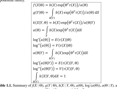
Where V(τ(X) | Y, Θ) is central covariance matrix of τ(X) given observed Y. Table 1.1 is summary of f(X | Θ), g(Y | Θ), k(X | Y, Θ), a(Θ), log’(a(Θ)), a(Θ | Y), and log’(a(Θ | Y)) with exponential family.
𝑓(𝑋|Θ) = 𝑏(𝑋) exp(Θ𝑇𝜏(𝑋)) 𝑎(Θ)⁄
𝑔(𝑌|Θ) = ∫ 𝑏(𝑋) exp(Θ𝑇𝜏(𝑋)) 𝑎(Θ)⁄ d𝑋 𝑿(𝑌)
𝑘(𝑋|𝑌, Θ) = 𝑏(𝑋) exp(Θ𝑇𝜏(𝑋)) 𝑎(Θ|𝑌)⁄
𝑎(Θ) = ∫ 𝑏(𝑋)exp(Θ𝑇𝜏(𝑋))d𝑋 𝑋
log′(𝑎(Θ)) = 𝐸(𝜏(𝑋)|Θ) log′′(𝑎(Θ)) = 𝑉(𝜏(𝑋)|Θ)
𝑎(Θ|𝑌) = ∫ 𝑏(𝑋)exp(Θ𝑇𝜏(𝑋))d𝑋
𝑿(𝑌)
log′(𝑎(Θ|𝑌)) = 𝐸(𝜏(𝑋)|𝑌, Θ) log′′(𝑎(Θ|𝑌)) = 𝑉(𝜏(𝑋)|𝑌, Θ)
∫ 𝑘(𝑋|𝑌, Θ)d𝑋 𝑿(𝑌)
= 1
Table 1.1. Summary of f(X | Θ), g(Y | Θ), k(X | Y, Θ), a(Θ), log’(a(Θ)), a(Θ | Y), and log’(a(Θ | Y)) with exponential family.
Simply, EM algorithm is iterative process including many iterations, in which each iteration has expectation step (E-step) and maximization step (M-step). E-step aims to estimate sufficient statistic given current parameter and observed data Y whereas M-step aims to re-estimate the parameter based on such sufficient statistic by maximizing likelihood function of X. EM algorithm is described in the next section in detail. As an introduction, DLR gave an example for illustrating EM algorithm (Dempster, Laird, & Rubin, 1977, pp. 2-3). Rao (Rao, 1955) presents observed data (incomplete data) Y of 197 animals following multinomial distribution with four categories, such as Y = (y1, y2, y3, y4) = (125, 18, 20, 34). The probability density function of Y is:
𝑔(𝑌|𝜃) = (∑ 𝑦𝑖 4
𝑖=1 )!
∏4𝑖=1𝑦𝑖! ∗ (1
2+ 𝜃 4)
𝑦1
∗ (1 4−
𝜃 4)
𝑦2
∗ (1 4−
𝜃 4)
𝑦3
∗ (𝜃 4)
𝑦4
Note, probabilities py1, py2, py3, and py4 in g(Y | θ) are 1/2 + θ/4, 1/4 – θ/4, 1/4 – θ/4, and θ/4, respectively as parameters. The expectation of any sufficient statistic yi with regard to g(Y | θ) is:
6 Observed data (incomplete data) Y is associated with hidden data X following multinomial distribution with five categories, such as X = {x1, x2, x3, x4, x5} where y1 = x1 + x2, y2 = x3, y3 = x4, y4 = x5. The probability density function of X is:
𝑓(𝑋|𝜃) = (∑ 𝑥𝑖 5
𝑖=1 )!
∏5𝑖=1(𝑥𝑖!) ∗ (1
2) 𝑥1
∗ (𝜃 4)
𝑥2
∗ (1 4−
𝜃 4)
𝑥3
∗ (1 4−
𝜃 4)
𝑥4
∗ (𝜃 4)
𝑥5
Note, probabilities px1, px2, px3, px4, and px5 in f(X | θ) are 1/2, θ/4, 1/4 – θ/4, 1/4 – θ/4, and θ/4, respectively as parameters. The expectation of any sufficient statistic xi with regard to f(X | θ) is:
𝐸(𝑥𝑖|𝜃) = 𝑥𝑖𝑝𝑥𝑖
Due to y1 = x1 + x2, y2 = x3, y3 = x4, y4 = x5, the mapping function φ between X and Y is y1 = φ(x1, x2) = x1 + x2. Therefore g(Y | θ) is sum of f(X | θ) over x1 and x2 such that x1 + x2 = y1 according to equation 1.1. In other words, g(Y | θ) is resulted from summing f(X | θ) over all (x1, x2) pairs such as (0, 125), (1, 124),…, (125, 0) because of y1 = 125 from observed Y.
𝑔(𝑌|𝜃) = ∑ ( ∑ 𝑓(𝑋|𝜃)
0
𝑥2=125−𝑥1
) 125
𝑥1=0
Rao (Rao, 1955) applied EM algorithm into determining the optimal estimate θ*. Note y2 = x3, y3 = x4, y4 = x5 are known and so only sufficient statistics x1 and x2 are not known. Given the tth iteration, sufficient statistics x1 and x2 are estimated as x1(t) and x2(t) based on current parameter θ(t) and g(Y | θ) in E-step below:
𝑥1(𝑡)+ 𝑥2(𝑡) = 𝑦1(𝑡) = 𝐸(𝑦1|𝑌, 𝜃(𝑡))
Due to y1 = 125 from observed data and py1 = 1/2 + θ/4, which implies that:
𝑥1(𝑡)+ 𝑥2(𝑡) = 𝐸(𝑦1|𝑌, 𝜃(𝑡)) = 𝑦1𝑝𝑦1 = 125 (1 2+
𝜃(𝑡) 4 )
We select:
𝑥1(𝑡) = 125 1 2⁄ 1 2⁄ + 𝜃(𝑡)⁄4
𝑥2(𝑡) = 125 𝜃 (𝑡)⁄4
1 2⁄ + 𝜃(𝑡)⁄4
According to M-step, the next estimate θ(t+1) is a maximizer of the log-likelihood function of X. This log-likelihood function is:
log(𝑓(𝑋|𝜃)) = log ((∑ 𝑥𝑖 5
𝑖=1 )!
∏5𝑖=1(𝑥𝑖!)) − (𝑥1 + 2𝑥2 + 2𝑥3+ 2𝑥4+ 2𝑥5)log(2) + (𝑥2 + 𝑥5)log(𝜃) + (𝑥3 + 𝑥4)log(1 − 𝜃)
The first-order derivative of log(f(X | θ) is:
dlog(𝑓(𝑋|𝜃))
d𝜃 =
𝑥2+ 𝑥5
𝜃 −
𝑥3 + 𝑥4 1 − 𝜃 =
𝑥2 + 𝑥5− (𝑥2+ 𝑥3+ 𝑥4+ 𝑥5)𝜃 𝜃(1 − 𝜃)
Because y2 = x3 = 18, y3 = x4 = 20, y4 = x5 = 34 and x2 is approximated by x2(t), we have:
𝜕log(𝑓(𝑋|𝜃))
𝜕𝜃 =
𝑥2(𝑡) + 34 − (𝑥2(𝑡)+ 72)𝜃
𝜃(1 − 𝜃)
As a maximizer of log(f(X | θ), the next estimate θ(t+1) is solution of the following equation
𝜕log(𝑓(𝑋|𝜃))
𝜕𝜃 =
𝑥2(𝑡)+ 34 − (𝑥2(𝑡) + 72)𝜃
𝜃(1 − 𝜃) = 0
7
𝜃(𝑡+1) =𝑥2 (𝑡)
+ 34
𝑥2(𝑡)+ 72
For example, given the initial θ(1) = 0.5, at the first iteration, we have:
𝑥2(1) = 125 𝜃 (0)⁄4
1 2⁄ + 𝜃(0)⁄4=
125 ∗ 0.5/4 0.5 + 0.5/4 = 25
𝜃(2) =𝑥2 (1)
+ 34
𝑥2(1)+ 72=
25 + 34
25 + 72 = 0.6082
After five iterations we gets the optimal estimate θ*:
𝜃∗ = 𝜃(4) = 𝜃(5)= 0.6268
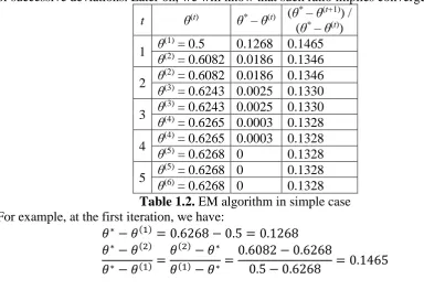
Table 1.2 (Dempster, Laird, & Rubin, 1977, p. 3) lists estimates of θ over five iterations (t =1, 2, 3, 4, 5) with note that θ(1) is initialized arbitrarily and θ* = θ(5) = θ(6) is determined at the 5th iteration. The third column gives deviation θ* and θ(t) whereas the fourth column gives the ratio of successive deviations. Later on, we will know that such ratio implies convergence rate.
t θ(t) θ* – θ(t) (θ
* – θ(t+1)) / (θ* – θ(t)) 1 θ
(1) = 0.5 0.1268 0.1465 θ(2) = 0.6082 0.0186 0.1346 2 θ
(2) = 0.6082 0.0186 0.1346 θ(3) = 0.6243 0.0025 0.1330 3 θ
(3) = 0.6243 0.0025 0.1330 θ(4) = 0.6265 0.0003 0.1328 4 θ
(4) = 0.6265 0.0003 0.1328 θ(5) = 0.6268 0 0.1328 5 θ
(5) = 0.6268 0 0.1328 θ(6) = 0.6268 0 0.1328
Table 1.2. EM algorithm in simple case For example, at the first iteration, we have:
𝜃∗− 𝜃(1)= 0.6268 − 0.5 = 0.1268 𝜃∗− 𝜃(2)
𝜃∗− 𝜃(1)=
𝜃(2)− 𝜃∗ 𝜃(1)− 𝜃∗ =
0.6082 − 0.6268
0.5 − 0.6268 = 0.1465
2. EM algorithm
Expectation maximization (EM) algorithm has many iterations and each iteration has two steps in which expectation step (E-step) calculates sufficient statistic of hidden data based on observed data and current parameter whereas maximization step (M-step) re-estimates parameter. When DLR proposed EM algorithm (Dempster, Laird, & Rubin, 1977), they firstly concerned that the probability density function f(X | Θ) of hidden space belongs to exponential family. E-step and M-step at the tth iteration are described in table 2.1 (Dempster, Laird, & Rubin, 1977, p. 4), in which the current estimate is Θ(t).
E-step:
We calculate current value τ(t) of the sufficient statistic τ(X) from observed Y and current parameter Θ(t) as follows:
𝜏(𝑡) = 𝐸(𝜏(𝑋)|𝑌, Θ(𝑡))
M-step:
Basing on τ(t), we determine the next parameter Θ(t+1) as solution of following equation:
𝐸(𝜏(𝑋)|Θ) = 𝜏(𝑡)
8
Table 2.1. E-step and M-step of EM algorithm
EM algorithm stops if two successive estimates are equal, Θ* = Θ(t) = Θ(t+1), at some tth iteration. At that time we conclude that Θ* is the optimal estimate of EM process. Please see table 1.1 to know how to calculate E(τ(X) | Θ(t)) and E(τ(X) | Y, Θ(t)).
It is necessary to explain E-step and M-step as well as convergence of EM algorithm. Essentially, the two steps aim to maximize log-likelihood function of Θ, denoted L(Θ), with respect to observation Y.
Θ∗ = argmax Θ
𝐿(Θ)
Where,
𝐿(Θ) = log(𝑔(𝑌|Θ))
Note that log(.) denotes logarithm function. Therefore, EM algorithm is an extension of maximum likelihood estimation (MLE) method. In fact, let l(Θ) be log-likelihood function of Θ with respect to variable X.
𝑙(Θ) = log(𝑓(𝑌|Θ)) = 𝑏(𝑋) exp(Θ𝑇𝜏(𝑋)) 𝑎(Θ)⁄ = log(𝑋) + Θ𝑇𝜏(𝑋) − log(𝑎(Θ))
By referring to table 1.1, the first-order derivative of l(Θ) is:
d𝑙(Θ)
dΘ =
dlog(𝑓(𝑌|Θ))
dΘ = 𝜏(𝑋) − log
′(𝑎(Θ)) = 𝜏(𝑋) − 𝐸(𝜏(𝑋)|Θ) (2.1)
Maximizing l(Θ) is to set the first-order derivative of l(Θ) to be zero. Therefore, the optimal estimate Θ* is solution of the following equation which is specified in M-step.
𝐸(𝜏(𝑋)|Θ) = 𝜏(𝑋)
The expression E(τ(X) | Θ) is function of Θ but τ(X) is still dependent on X. Let τ(t) be value of τ(X) at the tth iteration of EM process, candidate for the best estimate of Θ is solution of equation 2.2 according to M-step.
𝐸(𝜏(𝑋)|Θ) = 𝜏(𝑡) (2.2)
Thus, we will calculate τ(t) by maximizing the log-likelihood function L(Θ) with respect to observation Y. Recall that maximizing L(Θ) is the ultimate purpose of EM algorithm.
Θ∗ = argmax Θ
𝐿(Θ)
Where,
𝐿(Θ) = log(𝑔(𝑌|Θ)) = log ( ∫ 𝑓(𝑋|Θ)d𝑋 𝑿(𝑌)
) (2.3)
Due to:
𝑘(𝑋|𝑌, Θ) =𝑓(𝑋|Θ) 𝑔(𝑌|Θ)
It implies:
𝐿(Θ) = log(𝑔(𝑌|Θ)) = log(𝑓(𝑋|Θ)) − log(𝑘(𝑋|𝑌, Θ))
Because f(X | Θ) belongs to exponential family, we have:
𝑓(𝑋|Θ) = 𝑏(𝑋) exp(Θ𝑇𝜏(𝑋)) 𝑎(Θ)⁄ 𝑘(𝑋|𝑌, Θ) = 𝑏(𝑋) exp(Θ𝑇𝜏(𝑋)) 𝑎(Θ|𝑌)⁄
The log-likelihood function L(Θ) is reduced as follows:
𝐿(Θ) = −log(𝑎(Θ)) + log(𝑎(Θ|𝑌))
By referring to table 1.1, the first-order derivative of L(Θ) is:
d𝐿(Θ)
dΘ = −log
′(𝑎(Θ)) + log′(𝑎(Θ|𝑌)) = −𝐸(𝜏(𝑋)|Θ) + 𝐸(𝜏(𝑋)|𝑌, Θ) (2.4)
Maximizing L(Θ) is to set the first-order derivative of L(Θ) to be zero as be zero as follows:
−𝐸(𝜏(𝑋)|Θ) + 𝐸(𝜏(𝑋)|𝑌, Θ) = 0
9
𝐸(𝜏(𝑋)|Θ) = 𝐸(𝜏(𝑋)|𝑌, Θ)
Let Θ(t) be the current estimate at some tth iteration of EM process. Derived from the equality above, the value τ(t) is calculated as seen in equation 2.5.
𝜏(𝑡) = 𝐸(𝜏(𝑋)|𝑌, Θ(𝑡)) (2.5)
Equation 2.5 specifies the E-step of EM process. After t iterations we will obtain Θ* = Θ(t+1) = Θ(t) such that E(τ(X) | Y, Θ(t)) = E(τ(X) | Y, Θ*) = τ(t) = E(τ(X) | Θ*) = E(τ(X) | Θ(t+1)) when Θ(t+1) is solution of equation 2.2 (Dempster, Laird, & Rubin, 1977, p. 5). This means that Θ* is the optimal estimate of EM process because Θ* is solution of the equation:
𝐸(𝜏(𝑋)|Θ) = 𝐸(𝜏(𝑋)|𝑌, Θ)
Thus, we conclude that Θ* is the optimal estimate of EM process.
Θ∗ = argmax Θ
𝐿(Θ)
For further research, DLR gave a preeminent generality of EM algorithm (Dempster, Laird, & Rubin, 1977, pp. 6-11) in which f(X | Θ) specifies arbitrary distribution. In other words, there is no requirement of exponential family. They define the conditional expectation Q(Θ’ | Θ) according to equation 2.6 (Dempster, Laird, & Rubin, 1977, p. 6).
𝑄(Θ′|Θ) = 𝐸(log(𝑓(𝑋|Θ′))|𝑌, Θ) = ∫ 𝑘(𝑋|𝑌, Θ)log(𝑓(𝑋|Θ′))d𝑋 𝑿(𝑌)
(2.6) The two steps of generalized EM (GEM) algorithm aim to maximize Q(Θ | Θ(t)) at some tth iteration as seen in table 2.2 (Dempster, Laird, & Rubin, 1977, p. 6).
E-step:
The expectation Q(Θ | Θ(t)) is determined based on current Θ(t), according to equation 2.6.
M-step:
The next parameter Θ(t+1) is a maximizer of Q(Θ | Θ(t)). Note that Θ(t+1) will become current parameter at the next iteration ((t+1)th iteration).
Table 2.2. E-step and M-step of GEM algorithm
DLR proved that GEM algorithm converges at some tth iteration. At that time, Θ* = Θ(t+1) = Θ(t) is the optimal estimate of EM process. It is deduced from E-step and M-step that Q(Θ | Θ(t)) is increased after every iteration. How to maximize Q(Θ | Θ(t)) is optimization problem which is dependent on applications. For example, some popular methods to solve optimization problem are Newton-Raphson (Burden & Faires, 2011, pp. 67-71), gradient descent (Ta, 2014), and Lagrangian duality (Jia, 2013). GEM algorithm still aims to maximize the log-likelihood function L(Θ) specified by equation 2.3. The next section focuses on the convergence of GEM algorithm proved by DLR (Dempster, Laird, & Rubin, 1977, pp. 7-10) but firstly we should discuss some features of Q(Θ’ | Θ). In special case of exponential family, Q(Θ’ | Θ) is modified by equation 2.7.
𝑄(Θ′|Θ) = 𝐸(log(𝑏(𝑋))|𝑌, Θ) + (Θ′)𝑇𝜏
Θ− log(𝑎(Θ′)) (2.7)
Where,
𝐸(log(𝑏(𝑋))|𝑌, Θ) = ∫ 𝑘(𝑋|𝑌, Θ)log(𝑏(𝑋))d𝑋 𝑿(𝑌)
𝜏Θ = ∫ 𝑘(𝑋|𝑌, Θ)𝜏(𝑋)d𝑋 𝑿(𝑌)
Following is a proof of equation 2.7.
𝑄(Θ′|Θ) = 𝐸(log(𝑓(𝑋|Θ′))|𝑌, Θ)
10
= ∫ 𝑘(𝑋|𝑌, Θ) (log(𝑏(𝑋)) + (Θ′)𝑇𝜏(𝑋) − log(𝑎(Θ′))) d𝑋 𝑿(𝑌)
= ∫ 𝑘(𝑋|𝑌, Θ)log(𝑏(𝑋))d𝑋 𝑿(𝑌)
+ ∫ 𝑘(𝑋|𝑌, Θ)(Θ′)𝑇𝜏(𝑋)d𝑋 𝑿(𝑌)
− ∫ 𝑘(𝑋|𝑌, Θ) 𝑿(𝑌)
log(𝑎(Θ′))d𝑋
= 𝐸(log(𝑏(𝑋))|𝑌, Θ) + (Θ′)𝑇 ∫ 𝑘(𝑋|𝑌, Θ)𝜏(𝑋)d𝑋
𝑿(𝑌)
− log(𝑎(Θ′))
= 𝐸(log(𝑏(𝑋))|𝑌, Θ) + (Θ′)𝑇𝐸(𝜏(𝑋)|𝑌, Θ) − log(𝑎(Θ′))
Because k(X | Y, Θ) belongs exponential family, the expectation E(τ(X) | Y, Θ) is function of Θ, denoted τΘ. It implies:
𝑄(Θ′|Θ) = 𝐸(log(𝑏(𝑋))|𝑌, Θ) + (Θ′)𝑇𝜏
Θ− log(𝑎(Θ′))∎
If there is no mapping function φ: X → Y, the equation 2.6 is modified with assumption that there is a joint probability of X and Y, denoted P(X, Y | Θ). Note that P(X, Y | Θ) can be discrete or continuous. The condition probability of X given Y is specified according to Bayes’ rule as follows:
𝑃(𝑋|𝑌, Θ) = 𝑃(𝑋, 𝑌|Θ) ∫𝑋∈𝑿 𝑃(𝑋, 𝑌|Θ)d𝑋
0
Note, 𝑿0 ⊆ 𝑿 is domain of X. Given Y, we always have:
∫ 𝑃(𝑋|𝑌, Θ)d𝑋
𝑋∈𝑿0
= 1
Equation 2.8 specifies the conditional expectation Q(Θ’ | Θ) without mapping function.
𝑄(Θ′|Θ) = ∫ 𝑃(𝑋|𝑌, Θ)log(𝑃(𝑋, 𝑌|Θ′))d𝑋 𝑋∈𝑿0
(2.8) Note, the requirement of joint probability is stricter than requirement of mapping function φ and so, equation 2.6 is the most general definition of Q(Θ’ | Θ).
3. Convergence of EM algorithm
Recall that DLR proposed GEM algorithm which aims to maximize the log-likelihood function L(Θ) by maximizing Q(Θ’ | Θ) over many iterations. This section focuses on mathematical explanation of the convergence of GEM algorithm given by DLR (Dempster, Laird, & Rubin, 1977, pp. 6-9). Recall that we have:
𝐿(Θ) = log(𝑔(𝑌|Θ)) = log ( ∫ 𝑓(𝑋|Θ)d𝑋 𝑿(𝑌)
)
𝑄(Θ′|Θ) = 𝐸(log(𝑓(𝑋|Θ′))|𝑌, Θ) = ∫ 𝑘(𝑋|𝑌, Θ)log(𝑓(𝑋|Θ′))d𝑋 𝑿(𝑌)
Let H(Θ’ | Θ) be another conditional expectation which has strong relationship with Q(Θ’ | Θ) (Dempster, Laird, & Rubin, 1977, p. 6).
𝐻(Θ′|Θ) = 𝐸(log(𝑘(𝑋|𝑌, Θ′))|𝑌, Θ) = ∫ 𝑘(𝑋|𝑌, Θ)log(𝑘(𝑋|𝑌, Θ′))d𝑋
𝑿(𝑌)
(3.1) From equation 2.6 and equation 3.1, we have:
𝑄(Θ′|Θ) = 𝐿(Θ′) + 𝐻(Θ′|Θ) (3.2)
Following is a proof of equation 3.2.
𝑄(Θ′|Θ) = ∫ 𝑘(𝑋|𝑌, Θ)log(𝑓(𝑋|Θ′))d𝑋
𝑿(𝑌)
= ∫ 𝑘(𝑋|𝑌, Θ)log(𝑔(𝑌|Θ′)𝑘(𝑋|𝑌, Θ′))d𝑋
11
= ∫ 𝑘(𝑋|𝑌, Θ)log(𝑔(𝑌|Θ′))d𝑋 𝑿(𝑌)
+ ∫ 𝑘(𝑋|𝑌, Θ)log(𝑘(𝑋|𝑌, Θ′))d𝑋 𝑿(𝑌)
= log(𝑔(𝑌|Θ′)) ∫ 𝑘(𝑋|𝑌, Θ)d𝑋 𝑿(𝑌)
+ 𝐻(Θ′|Θ) = log(𝑔(𝑌|Θ′)) + 𝐻(Θ′|Θ)
= 𝐿(Θ′) + 𝐻(Θ′|Θ)∎
Lemma 1 (Dempster, Laird, & Rubin, 1977, p. 6). For any pair (Θ’, Θ) in Ω x Ω,
𝐻(Θ′|Θ) ≤ 𝐻(Θ|Θ) (3.3)
The equality occurs if and only if k(X | Y, Θ’) = k(X | Y, Θ) almost everywhere ■
Following is a proof of lemma 1 as well as equation 3.3. The log-likelihood function L(Θ’) is re-written as follows:
𝐿(Θ′) = log ( ∫ 𝑓(𝑋|Θ′)d𝑋
𝑿(𝑌)
) = log ( ∫ 𝑘(𝑋|𝑌, Θ) 𝑓(𝑋|Θ ′)
𝑘(𝑋|𝑌, Θ)d𝑋 𝑿(𝑌)
)
Due to
∫ 𝑘(𝑋|𝑌, Θ′)d𝑋
𝑿(𝑌)
= 1
By applying Jensen’s inequality (Sean, 2009, pp. 3-4) with concavity of logarithm function, Sean (Sean, 2009, p. 6) proved that:
𝐿(Θ′) ≥ ∫ 𝑘(𝑋|𝑌, Θ)log ( 𝑓(𝑋|Θ ′)
𝑘(𝑋|𝑌, Θ)) d𝑋 𝑿(𝑌)
= ∫ 𝑘(𝑋|𝑌, Θ) (log(𝑓(𝑋|Θ′)) − log(𝑘(𝑋|𝑌, Θ))) d𝑋 𝑿(𝑌)
= ∫ 𝑘(𝑋|𝑌, Θ)log(𝑘(𝑋|𝑌, Θ′)𝑔(𝑌|Θ′))d𝑋 𝑿(𝑌)
− ∫ 𝑘(𝑋|𝑌, Θ)log(𝑘(𝑋|𝑌, Θ))d𝑋 𝑿(𝑌)
= ∫ 𝑘(𝑋|𝑌, Θ) (log(𝑘(𝑋|𝑌, Θ′)) + log(𝑔(𝑌|Θ′))) d𝑋 𝑿(𝑌)
− 𝐻(Θ|Θ)
= ∫ 𝑘(𝑋|𝑌, Θ) (log(𝑘(𝑋|𝑌, Θ′))) d𝑋 𝑿(𝑌)
+ ∫ 𝑘(𝑋|𝑌, Θ) (log(𝑔(𝑌|Θ′))) d𝑋 𝑿(𝑌)
− 𝐻(Θ|Θ)
= 𝐻(Θ′|Θ) + log(𝑔(𝑌|Θ′)) ∫ 𝑘(𝑋|𝑌, Θ)d𝑋 𝑿(𝑌)
− 𝐻(Θ|Θ)
= 𝐻(Θ′|Θ) + 𝐿(Θ′) − 𝐻(Θ|Θ)
It implies:
𝐻(Θ′|Θ) ≤ 𝐻(Θ|Θ)∎
According to Jensen’s inequality (Sean, 2009, pp. 3-4), the equality occurs if and only if k(X | Y, Θ’) is linear or f(X | Θ’) is constant. In other words, the equality occurs if and only if k(X | Y, Θ’) = k(X | Y, Θ) almost everywhere when f(X | Θ) is not constant.
Let {Θ(𝑡)} 𝑡=1 +∞
= Θ(1), Θ(2), … , Θ(𝑡), Θ(𝑡+1), … be a sequence of estimates of Θ resulted from iterations of EM algorithm. Let Θ → M(Θ) be the mapping such that each estimation Θ(t) → Θ(t+1) at any given iteration is defined by equation 3.4 (Dempster, Laird, & Rubin, 1977, p. 7).
Θ(𝑡+1) = 𝑀(Θ(𝑡)) (3.4)
Definition1 (Dempster, Laird, & Rubin, 1977, p. 7). An iterative algorithm with mapping M(Θ)
is a GEM algorithm if
12 Of course, specification of GEM shown in table 2.2 satisfies the definition 1 because Θ(t+1) is a maximizer of Q(Θ | Θ(t)) with regard to variable Θ in M-step.
𝑄(𝑀(Θ(𝑡))|Θ(𝑡)) = 𝑄(Θ(𝑡+1)|Θ(𝑡)) ≥ 𝑄(Θ(𝑡)|Θ(𝑡)), ∀𝑡 Theorem 1 (Dempster, Laird, & Rubin, 1977, p. 7). For every GEM algorithm
𝐿(𝑀(Θ)) ≥ 𝐿(Θ) for all Θ ∈ Ω (3.6)
Where equality occurs if and only if Q(M(Θ) | Θ) = Q(Θ | Θ) and k(X | Y, M(Θ)) = k(X | Y, Θ) almost everywhere ■
Following is the proof of theorem 1 (Dempster, Laird, & Rubin, 1977, p. 7):
𝐿(𝑀(Θ)) − 𝐿(Θ) = (𝑄(𝑀(Θ)|Θ) − 𝐻(𝑀(Θ)|Θ)) − (𝑄(Θ|Θ) − 𝐻(Θ|Θ)) = (𝑄(𝑀(Θ)|Θ) − 𝑄(Θ|Θ)) + (𝐻(Θ|Θ) − 𝐻(𝑀(Θ)|Θ)) ≥ 0∎
Because the equality of lemma 1 occurs if and only if k(X | Y, Θ’) = k(X | Y, Θ) almost everywhere and the equality of the definition 1 is Q(M(Θ) | Θ) = Q(Θ | Θ), we deduce that the equality of theorem 1 occurs if and only if Q(M(Θ) | Θ) = Q(Θ | Θ) and k(X | Y, M(Θ)) = k(X | Y, Θ) almost everywhere. It is easy to draw corollary 1 and corollary 2 from definition 1 and theorem 1.
Corollary 1 (Dempster, Laird, & Rubin, 1977). Suppose for some Θ∗ ∈ Ω, L(Θ*) ≥ L(Θ) for all Θ ∈ Ω then for every GEM algorithm:
(a) L(M(Θ*)) = L(Θ*)
(b) Q(M(Θ*) | Θ*) = Q(Θ* | Θ*) (c) k(X | Y, M(Θ*)) = k(X | Y, Θ*) ■
Proof. From theorem 1 and the assumption of corollary 1, we have:
{𝐿(𝑀(Θ)) ≥ 𝐿(Θ) for all Θ ∈ Ω 𝐿(Θ∗) ≥ 𝐿(Θ) for all Θ ∈ Ω
This implies:
{𝐿(𝑀(Θ
∗)) ≥ 𝐿(Θ∗)
𝐿(𝑀(Θ∗)) ≤ 𝐿(Θ∗)
As a result,
𝐿(𝑀(Θ∗)) = 𝐿(𝑀(Θ∗))
From theorem 1, we also have:
𝑄(𝑀(Θ∗)|Θ∗) = 𝑄(Θ∗|Θ∗) 𝑘(𝑋|𝑌, 𝑀(Θ∗)) = 𝑘(𝑋|𝑌, Θ∗)∎
Corollary 2 (Dempster, Laird, & Rubin, 1977). If for some Θ∗∈ Ω, L(Θ*) > L(Θ) for all Θ ∈ Ω such that Θ ≠ Θ*, then for every GEM algorithm:
M(Θ*) = Θ* ■
Proof. From corollary 1 and the assumption of corollary 2, we have:
{𝐿(𝑀(Θ
∗)) = 𝐿(Θ∗)
𝐿(Θ∗) > 𝐿(Θ) for all Θ ∈ Ω and Θ ≠ Θ∗
If M(Θ*) ≠ Θ*, there is a contradiction L(M(Θ*)) = L(Θ*) > L(M(Θ*)). Therefore, we have M(Θ*) = Θ* ■
Theorem 2 (Dempster, Laird, & Rubin, 1977, p. 7). Suppose {Θ(𝑡)} 𝑡=1 +∞
is the sequence of estimates resulted from GEM algorithm such that:
(1) The sequence {𝐿(Θ(𝑡))}𝑡=1+∞ = 𝐿(Θ(1)), 𝐿(Θ(2)), … , 𝐿(Θ(𝑡)), … is bounded above, and (2) Q(Θ(t+1) | Θ(t)) – Q(Θ(t) | Θ(t)) ≥ ξ(Θ(t+1) – Θ(t))T(Θ(t+1) – Θ(t)) for some scalar ξ > 0 and all
t.
13 Proof. The sequence {𝐿(Θ(𝑡))}
𝑡=1 +∞
is non-decreasing according to theorem 1 and is bounded above according to the assumption 1 of theorem 2 and hence, the sequence {𝐿(Θ(𝑡))}
𝑡=1 +∞
converges to some L* < +∞. According to Cauchy criterion (Dinh, Pham, Nguyen, & Ta, 2000, p. 34), for all ε > 0, there exists a t(ε) such that, for all t ≥ t(ε) and all v ≥ 1:
𝐿(Θ(𝑡+𝑣)) − 𝐿(Θ(𝑡)) = ∑ (𝐿(Θ(𝑡+𝑖)) − 𝐿(Θ(𝑡+𝑖−1))) 𝑣
𝑖=1
< 𝜀
By applying equations 3.2 and 3.3, for all i ≥ 1, we obtain:
𝑄(Θ(𝑡+𝑖)|Θ(𝑡+𝑖−1)) − 𝑄(Θ(𝑡+𝑖−1)|Θ(𝑡+𝑖−1))
= 𝐿(Θ(𝑡+𝑖)) + 𝐻(Θ(𝑡+𝑖)|Θ(𝑡+𝑖−1)) − 𝑄(Θ(𝑡+𝑖−1)|Θ(𝑡+𝑖−1))
≤ 𝐿(Θ(𝑡+𝑖)) + 𝐻(Θ(𝑡+𝑖−1)|Θ(𝑡+𝑖−1)) − 𝑄(Θ(𝑡+𝑖−1)|Θ(𝑡+𝑖−1)) = 𝐿(Θ(𝑡+𝑖)) − 𝐿(Θ(𝑡+𝑖−1))
(Due to L(Θ(t+i–1)) = Q(Θ(t+i–1) | Θ(t+i–1)) – H(Θ(t+i–1) | Θ(t+i–1)) according to equation 3.2) It implies
∑ (𝑄(Θ(𝑡+𝑖)|Θ(𝑡+𝑖−1)) − 𝑄(Θ(𝑡+𝑖−1)|Θ(𝑡+𝑖−1))) 𝑣
𝑖=1
< ∑ (𝐿(Θ(𝑡+𝑖)) − 𝐿(Θ(𝑡+𝑖−1))) 𝑣
𝑖=1 = 𝐿(Θ(𝑡+𝑣)) − 𝐿(Θ(𝑡)) < 𝜀
By applying v times the assumption 2 of theorem 2, we obtain:
𝜀 > ∑ (𝑄(Θ(𝑡+𝑖)|Θ(𝑡+𝑖−1)) − 𝑄(Θ(𝑡+𝑖−1)|Θ(𝑡+𝑖−1))) 𝑣
𝑖=1
≥ 𝜉 ∑(Θ(𝑡+𝑖)− Θ(𝑡+𝑖−1))𝑇(Θ(𝑡+𝑖)− Θ(𝑡+𝑖−1)) 𝑣
𝑖=1
It means that
∑|Θ(𝑡+𝑖)− Θ(𝑡+𝑖−1)|2 𝑣
𝑖=1
< 𝜀 𝜉⁄
Where,
|Θ(𝑡+𝑖)− Θ(𝑡+𝑖−1)|2 = (Θ(𝑡+𝑖)− Θ(𝑡+𝑖−1))𝑇(Θ(𝑡+𝑖)− Θ(𝑡+𝑖−1))
Notation |.| denotes length of vector and so |Θ(t+i) – Θ(t+i –1)| is distance between Θ(t+i) and Θ(t+i –1). Applying triangular inequality, for any ε > 0, for all t ≥ t(ε) and all v ≥ 1, we have:
|Θ(𝑡+𝑣)− Θ(𝑡)|2 < 𝜀 𝜉⁄
According to Cauchy criterion, the sequence {Θ(𝑡)} 𝑡=1 +∞
converges to some Θ* in the closure of Ω.
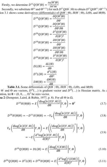
14 - Firstly, we determine 𝐷11𝑄(Θ′|Θ) = 𝜕𝑄(Θ
′|Θ)
𝜕Θ′𝜕Θ
- Secondly, we substitute Θ(t) and Θ(t+1)) for such D11Q(Θ’ | Θ) to obtain D11Q(Θ(t) | Θ(t+1)). Equation 3.1 shows some derivatives (differentials) of Q(Θ’ | Θ), H(Θ’ | Θ), L(Θ), and M(Θ).
𝐷10𝑄(Θ′|Θ) = 𝜕𝑄(Θ ′|Θ)
𝜕Θ′
𝐷11𝑄(Θ′|Θ) = 𝜕𝑄(Θ ′|Θ)
𝜕Θ′𝜕Θ
𝐷20𝑄(Θ′|Θ) =𝜕
2𝑄(Θ′|Θ)
𝜕(Θ′)2
𝐷10𝐻(Θ′|Θ) =𝜕𝐻(Θ ′|Θ)
𝜕Θ′
𝐷11𝐻(Θ′|Θ) =𝜕𝐻(Θ ′|Θ)
𝜕Θ′𝜕Θ
𝐷20𝐻(Θ′|Θ) =𝜕
2𝐻(Θ′|Θ)
𝜕(Θ′)2
𝐷𝐿(Θ) =d𝐿(Θ) dΘ
𝐷2𝐿(Θ) =d
2𝐿(Θ)
dΘ2
𝐷𝑀(Θ) =d𝑀(Θ) dΘ
Table 3.1. Some differentials of Q(Θ’ | Θ), H(Θ’ | Θ), L(Θ), and M(Θ)
When Θ’ and Θ are vectors, D10(…) is gradient vector and D20(…) is Hessian matrix. As a convention, let 0 = (0, 0,…, 0)T be zero vector.
Lemma 2 (Dempster, Laird, & Rubin, 1977, p. 8). For all Θ in Ω,
𝐷10𝐻(Θ|Θ) = 𝐸 (dlog(𝑘(𝑋|𝑌, Θ))
dΘ |𝑌, Θ) = 𝟎𝑇 (3.7)
𝐷20𝐻(Θ|Θ) = −𝐷11𝐻(Θ|Θ) = −𝑉
𝑁(
dlog(𝑘(𝑋|𝑌, Θ))
dΘ |𝑌, Θ) (3.8)
𝑉𝑁(dlog(𝑘(𝑋|𝑌, Θ))dΘ |𝑌, Θ) = 𝐸 ((dlog(𝑘(𝑋|𝑌, Θ))dΘ ) 2
|𝑌, Θ)
= −𝐸 (𝑑
2log(𝑘(𝑋|𝑌, Θ))
d(Θ)2 |𝑌, Θ)
(3.9)
𝐷10𝑄(Θ|Θ) = 𝐷𝐿(Θ) = 𝐸 (dlog(𝑓(𝑋|Θ))dΘ |𝑌, Θ) (3.10)
𝐷20𝑄(Θ|Θ) = 𝐷2𝐿(Θ) + 𝐷20𝐻(Θ|Θ) = 𝐸 (𝑑
2log(𝑓(𝑋|Θ))
15
𝑉𝑁(dlog(𝑓(𝑋|Θ))dΘ |𝑌, Θ) = 𝐸 ((dlog(𝑓(𝑋|Θ))dΘ ) 2
|𝑌, Θ)
= 𝐷2𝐿(Θ) + (𝐷𝐿(Θ))2− 𝐷20𝑄(Θ|Θ)∎
(3.12) Note, VN(.) denotes non-central covariance matrix. Followings are proofs of equations 3.7, 3.8, 3.9, 3.10, 3.11, and 3.12. In fact, we have:
𝐷10𝐻(Θ′|Θ) = 𝜕
𝜕Θ′𝐸(log(𝑘(𝑋|𝑌, Θ
′))|𝑌, Θ) = 𝜕
𝜕Θ′( ∫ 𝑘(𝑋|𝑌, Θ)log(𝑘(𝑋|𝑌, Θ ′))d𝑋
𝑿(𝑌)
)
= ∫ 𝑘(𝑋|𝑌, Θ)dlog(𝑘(𝑋|𝑌, Θ ′))
dΘ′ d𝑋
𝑿(𝑌)
= 𝐸 (dlog(𝑘(𝑋|𝑌, Θ ′))
dΘ′ |𝑌, Θ) =
= ∫ 𝑘(𝑋|𝑌, Θ) 𝑘(𝑋|𝑌, Θ′)
d(𝑘(𝑋|𝑌, Θ′))
dΘ′ d𝑋
𝑿(𝑌)
It implies:
𝐷10𝐻(Θ|Θ) = ∫ 𝑘(𝑋|𝑌, Θ) 𝑘(𝑋|𝑌, Θ)
d(𝑘(𝑋|𝑌, Θ))
dΘ d𝑋
𝑿(𝑌)
= d
dΘ( ∫ 𝑘(𝑋|𝑌, Θ)d𝑋 𝑿(𝑌)
) = d
dΘ(1) = 𝟎 𝑇
We also have:
𝐷11𝐻(Θ′|Θ) = 𝜕𝐷
10𝐻(Θ′|Θ)
𝜕Θ = ∫
1 𝑘(𝑋|𝑌, Θ′)
d𝑘(𝑋|𝑌, Θ) 𝑑Θ
d𝑘(𝑋|𝑌, Θ′)
dΘ′ d𝑋
𝑿(𝑌)
It implies:
𝐷11𝐻(Θ|Θ) = ∫ 1
𝑘(𝑋|𝑌, Θ) d𝑘(𝑋|𝑌, Θ) 𝑑Θ d𝑘(𝑋|𝑌, Θ) dΘ d𝑋 𝑿(𝑌)
= ∫ 𝑘(𝑋|𝑌, Θ) ( 1 𝑘(𝑋|𝑌, Θ) d𝑘(𝑋|𝑌, Θ) 𝑑Θ ) 2 d𝑋 𝑿(𝑌) = 𝑉𝑁( dlog(𝑘(𝑋|𝑌, Θ))
dΘ |𝑌, Θ)
We also have:
𝐷20𝐻(Θ′|Θ) =𝜕𝐷
10𝐻(Θ′|Θ)
𝜕Θ′ = 𝐸 (
𝑑2log(𝑘(𝑋|𝑌, Θ′)) d(Θ′)2 |𝑌, Θ)
= − ∫ 𝑘(𝑋|𝑌, Θ) (𝑘(𝑋|𝑌, Θ′))2(
d𝑘(𝑋|𝑌, Θ′)
dΘ′ )
2 d𝑋 𝑿(𝑌)
= −𝐸 ((dlog(𝑘(𝑋|𝑌, Θ))dΘ ) 2
|𝑌, Θ)
It implies:
𝐷20𝐻(Θ|Θ) = − ∫ 𝑘(𝑋|𝑌, Θ) ( 1 𝑘(𝑋|𝑌, Θ) d𝑘(𝑋|𝑌, Θ) 𝑑Θ ) 2 d𝑋 𝑿(𝑌) = −𝑉𝑁( dlog(𝑘(𝑋|𝑌, Θ))
dΘ |𝑌, Θ)
From equation 3.2, we have:
𝐷20𝑄(Θ′|Θ) = 𝐷2𝐿(Θ′) + 𝐷20𝐻(Θ′|Θ)
We also have:
𝐷10𝑄(Θ′|Θ) = 𝜕
𝜕Θ′( ∫ 𝑘(𝑋|𝑌, Θ)log(𝑓(𝑋|Θ′))d𝑋 𝑿(𝑌)
) = ∫ 𝑘(𝑋|𝑌, Θ)dlog(𝑓(𝑋|Θ ′))
dΘ′ d𝑋
16
= ∫ 𝑘(𝑋|𝑌, Θ)dlog(𝑓(𝑋|Θ ′))
dΘ′ d𝑋
𝑿(𝑌)
= 𝐸 (dlog(𝑓(𝑋|Θ ′))
dΘ′ |𝑌, Θ)
= ∫ 𝑘(𝑋|𝑌, Θ) 𝑓(𝑋|Θ′)
d𝑓(𝑋|Θ′) dΘ′ d𝑋 𝑿(𝑌)
It implies:
𝐷10𝑄(Θ|Θ) = ∫ 𝑘(𝑋|𝑌, Θ) 𝑓(𝑋|Θ)
d𝑓(𝑋|Θ)
dΘ d𝑋
𝑿(𝑌)
= ∫ 1
𝑔(𝑌|Θ) d𝑓(𝑋|Θ) dΘ d𝑋 𝑿(𝑌) = 1 𝑔(𝑌|Θ) ∫ d𝑓(𝑋|Θ) dΘ d𝑋 𝑿(𝑌) = 1 𝑔(𝑌|Θ) d
dΘ( ∫ 𝑓(𝑋|Θ)d𝑋 𝑿(𝑌) ) = 1 𝑔(𝑌|Θ) d𝑔(𝑌|Θ) dΘ = dlog(𝑔(𝑌|Θ))
dΘ = 𝐷𝐿(Θ)
We have:
𝐷20𝑄(Θ′|Θ) =𝜕𝐷
10𝑄(Θ′|Θ)
𝜕Θ′ =
𝜕 𝜕Θ′( ∫
𝑘(𝑋|𝑌, Θ) 𝑓(𝑋|Θ′)
d𝑓(𝑋|Θ′)
dΘ′ d𝑋
𝑿(𝑌)
)
= ∫ 𝑘(𝑋|𝑌, Θ) 𝑑 dΘ′(
d𝑓(𝑋|Θ′) dΘ⁄ ′ 𝑓(𝑋|Θ′) ) d𝑋 𝑿(𝑌)
= 𝐸 (𝑑
2log(𝑓(𝑋|Θ′))
d(Θ′)2 |𝑌, Θ)
= ∫ 𝑘(𝑋|𝑌, Θ) ((d2𝑓(𝑋|Θ′) d(Θ⁄ ′)2)𝑓(𝑋|Θ′) − (d𝑓(𝑋|Θ′) dΘ⁄ ′)2) (𝑓(𝑋|Θ⁄ ′))2d𝑋 𝑿(𝑌)
= ∫ 𝑘(𝑋|𝑌, Θ)(d
2𝑓(𝑋|Θ′) d(Θ⁄ ′)2)
𝑓(𝑋|Θ′) d𝑋
𝑿(𝑌)
− ∫ 𝑘(𝑋|𝑌, Θ) (d𝑓(𝑋|Θ ′) dΘ⁄ ′
𝑓(𝑋|Θ′) ) 2
d𝑋 𝑿(𝑌)
= ∫ 𝑘(𝑋|𝑌, Θ)(d
2𝑓(𝑋|Θ′) d(Θ⁄ ′)2)
𝑓(𝑋|Θ′) d𝑋
𝑿(𝑌)
− 𝑉𝑁(
dlog(𝑓(𝑋|Θ′))
dΘ′ |𝑌, Θ)
It implies:
𝐷20𝑄(Θ|Θ) = ∫ 𝑘(𝑋|𝑌, Θ)(d
2𝑓(𝑋|Θ) d(Θ)⁄ 2)
𝑓(𝑋|Θ) d𝑋
𝑿(𝑌)
− 𝑉𝑁(dlog(𝑓(𝑋|Θ))dΘ |𝑌, Θ)
= 1
𝑔(𝑌|Θ) ∫
d2𝑓(𝑋|Θ) d(Θ)2 d𝑋 𝑿(𝑌)
− 𝑉𝑁(dlog(𝑓(𝑋|Θ))
dΘ |𝑌, Θ)
= 1
𝑔(𝑌|Θ) d2
d(Θ)2( ∫
𝑓(𝑋|Θ)
dΘ d𝑋
𝑿(𝑌)
) − 𝑉𝑁(dlog(𝑓(𝑋|Θ))dΘ |𝑌, Θ)
= 1
𝑔(𝑌|Θ)
d2𝑔(𝑌|Θ)
d(Θ)2 − 𝑉𝑁(
dlog(𝑓(𝑋|Θ))
dΘ |𝑌, Θ)
Due to:
𝐷2𝐿(Θ) =d
2log(𝑔(𝑌|Θ))
d(Θ)2 =
1 𝑔(𝑌|Θ)
d2𝑔(𝑌|Θ)
d(Θ)2 − (𝐷𝐿(Θ)) 2
We have:
𝐷20𝑄(Θ|Θ) = 𝐷2𝐿(Θ) + (𝐷𝐿(Θ))2− 𝑉𝑁(
dlog(𝑓(𝑋|Θ))
17
Lemma 3 (Dempster, Laird, & Rubin, 1977, p. 9). If f(X | Θ) and k(X | Y, Θ) belong to exponential family, for all Θ in Ω, we have:
𝐷10𝐻(Θ′|Θ) = 𝐸(𝜏(𝑋)|𝑌, Θ) − 𝐸(𝜏(𝑋)|𝑌, Θ′) (3.13)
𝐷20𝐻(Θ′|Θ) = −𝑉(𝜏(𝑋)|𝑌, Θ′) (3.14)
𝐷10𝑄(Θ′|Θ) = 𝐸(𝜏(𝑋)|Θ) − 𝐸(𝜏(𝑋)|Θ′) (3.15)
𝐷20𝑄(Θ′|Θ) = −𝑉(𝜏(𝑋)|Θ′)∎ (3.16)
Proof. If f(X | Θ’) and k(X | Y, Θ’) belong to exponential family, from table 1.1 we have:
dlog(𝑓(𝑌|Θ′))
dΘ′ =
d
dΘ′(𝑏(𝑋) exp((Θ
′)𝑇𝜏(𝑋)) 𝑎(Θ⁄ ′)) = 𝜏(𝑋) − log′(𝑎(Θ′))
= 𝜏(𝑋) − 𝐸(𝜏(𝑋)|Θ′)
And,
d2log(𝑓(𝑌|Θ′)) d(Θ′)2 =
d
d(Θ′)2(𝑏(𝑋) exp((Θ′)𝑇𝜏(𝑋)) 𝑎(Θ⁄ ′)) = −log′′(𝑎(Θ′)) = −𝑉(𝜏(𝑋)|Θ′)
And,
dlog(𝑘(𝑌|Θ′))
dΘ′ =
d
dΘ′(𝑏(𝑋) exp((Θ′)𝑇𝜏(𝑋)) 𝑎(Θ⁄ ′|𝑌)) = 𝜏(𝑋) − log′(𝑎(Θ′)|𝑌) = 𝜏(𝑋) − 𝐸(𝜏(𝑋)|𝑌, Θ′)
And,
d2log(𝑘(𝑋|𝑌, Θ′)) d(Θ′)2 =
d
d(Θ′)2(𝑏(𝑋) exp((Θ
′)𝑇𝜏(𝑋)) 𝑎(Θ⁄ ′|𝑌)) = −log′′(𝑎(Θ′|𝑌))
= −𝑉(𝜏(𝑋)|𝑌, Θ′)
Hence,
𝐷10𝐻(Θ′|Θ) = 𝜕
𝜕Θ′( ∫ 𝑘(𝑋|𝑌, Θ)log(𝑘(𝑋|𝑌, Θ′))d𝑋 𝑿(𝑌)
)
= ∫ 𝑘(𝑋|𝑌, Θ)dlog(𝑘(𝑋|𝑌, Θ ′))
dΘ′ d𝑋
𝑿(𝑌)
= ∫ 𝑘(𝑋|𝑌, Θ)𝜏(𝑋)d𝑋
𝑿(𝑌)
− ∫ 𝑘(𝑋|𝑌, Θ)𝐸(𝜏(𝑋)|𝑌, Θ′)d𝑋
𝑿(𝑌)
= 𝐸(𝜏(𝑋)|𝑌, Θ) − 𝐸(𝜏(𝑋)|𝑌, Θ′) ∫ 𝑘(𝑋|𝑌, Θ)d𝑋 𝑿(𝑌)
= 𝐸(𝜏(𝑋)|𝑌, Θ) − 𝐸(𝜏(𝑋)|𝑌, Θ′)
We have:
𝐷20𝐻(Θ′|Θ) = 𝜕 2
𝜕(Θ′)2( ∫ 𝑘(𝑋|𝑌, Θ)log(𝑘(𝑋|𝑌, Θ′))d𝑋 𝑿(𝑌)
)
= ∫ 𝑘(𝑋|𝑌, Θ)d
2log(𝑘(𝑋|𝑌, Θ′))
d(Θ′)2 d𝑋 𝑿(𝑌)
= − ∫ 𝑘(𝑋|𝑌, Θ)log′′(𝑎(Θ′)|𝑌)d𝑋 𝑿(𝑌)
= −log′′(𝑎(Θ′)|𝑌) ∫ 𝑘(𝑋|𝑌, Θ)d𝑋 𝑿(𝑌)
= −log′′(𝑎(Θ′)|𝑌) = −𝑉(𝜏(𝑋)|𝑌, Θ′)
18
𝐷10𝑄(Θ′|Θ) = 𝜕
𝜕Θ′( ∫ 𝑘(𝑋|𝑌, Θ)log(𝑓(𝑋|Θ′))d𝑋 𝑿(𝑌)
) = ∫ 𝑘(𝑋|𝑌, Θ)dlog(𝑓(𝑋|Θ ′))
dΘ′ d𝑋
𝑿(𝑌)
= ∫ 𝑘(𝑋|𝑌, Θ)𝜏(𝑋)d𝑋 𝑿(𝑌)
− ∫ 𝑘(𝑋|𝑌, Θ)𝐸(𝜏(𝑋)|Θ)d𝑋 𝑿(𝑌)
= 𝐸(𝜏(𝑋)|Θ) − 𝐸(𝜏(𝑋)|Θ′) ∫ 𝑘(𝑋|𝑌, Θ)d𝑋 𝑿(𝑌)
= 𝐸(𝜏(𝑋)|Θ) − 𝐸(𝜏(𝑋)|Θ′)
We have:
𝐷20𝑄(Θ′|Θ) = 𝜕 2
𝜕(Θ′)2( ∫ 𝑘(𝑋|𝑌, Θ)log(𝑓(𝑋|Θ′))d𝑋 𝑿(𝑌)
)
= ∫ 𝑘(𝑋|𝑌, Θ)d
2log(𝑓(𝑋|Θ′))
d(Θ′)2 d𝑋 𝑿(𝑌)
= − ∫ 𝑘(𝑋|𝑌, Θ)log′′(𝑎(Θ′))d𝑋 𝑿(𝑌)
= −log′′(𝑎(Θ′)) ∫ 𝑘(𝑋|𝑌, Θ)d𝑋 𝑿(𝑌)
= −log′′(𝑎(Θ′)) = −𝑉(𝜏(𝑋)|Θ′)∎
Theorem 3 (Dempster, Laird, & Rubin, 1977, p. 8). Suppose the sequence {Θ(𝑡)} 𝑡=1 +∞
is an instance of GEM algorithm such that
𝐷10𝑄(Θ(𝑡+1)|Θ(𝑡)) = 𝟎𝑇
Then for all t, there exists a Θ0(t+1) on the line segment joining Θ(t) and Θ(t+1) such that
𝑄(Θ(𝑡+1)|Θ(𝑡)) − 𝑄(Θ(𝑡)|Θ(𝑡)) = −(Θ(𝑡+1)− Θ(𝑡))𝑇𝐷20𝑄(Θ0(𝑡+1)|Θ(𝑡))(Θ(𝑡+1)− Θ(𝑡))
Furthermore, if D20Q(Θ0(t+1) | Θ(t)) is negative definite, and the sequence {𝐿(Θ(𝑡))}𝑡=1+∞ is bounded above then, the sequence {Θ(𝑡)}
𝑡=1 +∞
converges to some Θ* in the closure of Ω ■ Note, if Θ is a scalar parameter, D20Q(Θ0(t+1) | Θ(t)) degrades as a scalar and the concept “negative definite” becomes “negative” simply. Following is a proof of theorem 3.
Proof. Second-order Taylor series expending for Q(Θ | Θ(t)) at Θ = Θ(t+1) to obtain:
𝑄(Θ|Θ(𝑡)) = 𝑄(Θ(𝑡+1)|Θ(𝑡)) + 𝐷10𝑄(Θ(𝑡+1)|Θ(𝑡))(Θ − Θ(𝑡+1)) + (Θ − Θ(𝑡+1))𝑇𝐷20𝑄(Θ
0
(𝑡+1)|Θ(𝑡))(Θ − Θ(𝑡+1))
= 𝑄(Θ(𝑡+1)|Θ(𝑡)) + (Θ − Θ(𝑡+1))𝑇𝐷20𝑄(Θ0(𝑡+1)|Θ(𝑡))(Θ − Θ(𝑡+1)) (due to 𝐷10𝑄(Θ(𝑡+1)|Θ(𝑡)) = 𝟎𝑇)
Where Θ0(t+1) is on the line segment joining Θ and Θ(t+1). Let Θ = Θ(t), we have:
𝑄(Θ(𝑡+1)|Θ(𝑡)) − 𝑄(Θ(𝑡)|Θ(𝑡)) = −(Θ(𝑡+1)− Θ(𝑡))𝑇𝐷20𝑄(Θ0(𝑡+1)|Θ(𝑡))(Θ(𝑡+1)− Θ(𝑡))
If D20Q(Θ(t+1) | Θ(t)) is negative definite then,
𝑄(Θ(𝑡+1)|Θ(𝑡)) − 𝑄(Θ(𝑡)|Θ(𝑡)) = −(Θ(𝑡+1)− Θ(𝑡))𝑇𝐷20𝑄(Θ0(𝑡+1)|Θ(𝑡))(Θ(𝑡+1)− Θ(𝑡)) > 0
Whereas,
(Θ(𝑡+1)− Θ(𝑡))𝑇(Θ(𝑡+1)− Θ(𝑡)) ≥ 0
So there exists some ξ > 0 such that
𝑄(Θ(𝑡+1)|Θ(𝑡)) − 𝑄(Θ(𝑡)|Θ(𝑡)) ≥ 𝜉(Θ(𝑡+1)− Θ(𝑡))𝑇(Θ(𝑡+1)− Θ(𝑡))
In other words, the assumption 2 of theorem 2 is satisfied and hence, the sequence {Θ(𝑡)} 𝑡=1 +∞
converges to some Θ* in the closure of Ω if the sequence {𝐿(Θ(𝑡))} 𝑡=1 +∞
19
Theorem 4 (Dempster, Laird, & Rubin, 1977, p. 9). Suppose the sequence {Θ(𝑡)} 𝑡=1 +∞
is an instance of GEM algorithm such that
(1) The sequence {Θ(𝑡)} 𝑡=1 +∞
converges to Θ* in the closure of Ω. (2) D10Q(Θ(t+1) | Θ(t)) = 0T for all t.
(3) D20Q(Θ(t+1) | Θ(t)) is negative definite for all t. Then DL(Θ*) = 0T, D20Q(Θ* | Θ*) is negative definite, and
𝐷𝑀(Θ∗) = 𝐷20𝐻(Θ∗|Θ∗)(𝐷20𝑄(Θ∗|Θ∗))−1∎ (3.17)
The notation “–1” denotes inverse of matrix. Note, DM(Θ*) is differential of M(Θ) at Θ = Θ*, which implies convergence of GEM algorithm. Followings are proofs of theorem 4.
From equation 3.2, we have:
𝐷𝐿(Θ(𝑡+1)) = 𝐷10𝑄(Θ(𝑡+1)|Θ(𝑡)) − 𝐷10𝐻(Θ(𝑡+1)|Θ(𝑡)) = −𝐷10𝐻(Θ(𝑡+1)|Θ(𝑡)) (Due to 𝐷10𝑄(Θ(𝑡+1)|Θ(𝑡)) = 𝟎𝑇)
When t approaches +∞ such that Θ(t) = Θ(t+1) = Θ* then, D10H(Θ* | Θ*) is zero according to equation 3.7 and so we have:
DL(Θ*) = 0T
Of course, D20Q(Θ* | Θ*) is negative definite because D20Q(Θ(t+1) | Θ(t)) is negative definite, when t approaches +∞ such that Θ(t) = Θ(t+1) = Θ*.
By first-order Taylor series expansion for D10Q(Θ2 | Θ1) as a function of Θ1 at Θ1 = Θ* and as a function of Θ2 at Θ2 = Θ*, respectively, we have:
𝐷10𝑄(Θ
2|Θ1) = 𝐷10𝑄(Θ2|Θ∗) + (Θ1− Θ∗)𝑇𝐷11𝑄(Θ2|Θ∗) + 𝑅1(Θ1) 𝐷10𝑄(Θ2|Θ1) = 𝐷10𝑄(Θ∗|Θ1) + (Θ2− Θ∗)𝑇𝐷20𝑄(Θ∗|Θ1) + 𝑅2(Θ2)
Where R1(Θ1) and R2(Θ2) are remainders. By summing such two series, we have:
2𝐷10𝑄(Θ2|Θ1)
= 𝐷10𝑄(Θ2|Θ∗) + 𝐷10𝑄(Θ∗|Θ1) + (Θ1− Θ∗)𝑇𝐷11𝑄(Θ2|Θ∗) + (Θ2− Θ∗)𝑇𝐷20𝑄(Θ∗|Θ
1) + 𝑅1(Θ1) + 𝑅2(Θ2)
By substituting Θ1 = Θ(t) and Θ2 = Θ(t+1), we have:
2𝐷10𝑄(Θ(𝑡+1)|Θ(𝑡))
= 𝐷10𝑄(Θ(𝑡+1)|Θ∗) + 𝐷10𝑄(Θ∗|Θ(𝑡)) + (Θ(𝑡)− Θ∗)𝑇𝐷11𝑄(Θ(𝑡+1)|Θ∗) + (Θ(𝑡+1)− Θ∗)𝑇𝐷20𝑄(Θ∗|Θ(𝑡)) + 𝑅1(Θ(𝑡)) + 𝑅2(Θ(𝑡+1))
It implies:
(𝑀(Θ(𝑡)) − 𝑀(Θ∗))𝑇 = (Θ(𝑡+1)− Θ∗)𝑇
= −(Θ(𝑡)− Θ∗)𝑇𝐷11𝑄(Θ(𝑡+1)|Θ∗) (𝐷20𝑄(Θ∗|Θ(𝑡)))−1
− (𝐷10𝑄(Θ(𝑡+1)|Θ∗) + 𝐷10𝑄(Θ∗|Θ(𝑡))) (𝐷20𝑄(Θ∗|Θ(𝑡)))−1
− (𝑅1(Θ(𝑡)) + 𝑅2(Θ(𝑡+1))) (𝐷20𝑄(Θ∗|Θ(𝑡))) −1
Let t approach +∞ such that Θ(t) = Θ(t+1) = Θ*, we obtain DM(Θ*) as differential of M(Θ) at Θ* as follows:
𝐷𝑀(Θ∗) = −𝐷11𝑄(Θ∗|Θ∗)(𝐷20𝑄(Θ∗|Θ∗))−1 (3.18)
20
𝐷11𝑄(Θ(𝑡+1)|Θ∗) = 𝐷11𝑄(Θ∗|Θ∗) 𝐷20𝑄(Θ∗|Θ(𝑡)) = 𝐷20𝑄(Θ∗|Θ∗)
𝐷10𝑄(Θ(𝑡+1)|Θ∗) = 𝐷10𝑄(Θ∗|Θ∗) = 𝟎𝑇 𝐷10𝑄(Θ∗|Θ(𝑡)) = 𝐷10𝑄(Θ∗|Θ∗) = 𝟎𝑇
lim
𝑡→+∞𝑅1(Θ
(𝑡)) = lim
Θ(𝑡)→Θ∗𝑅1(Θ
(𝑡)) = 0
lim
𝑡→+∞𝑅2(Θ
(𝑡+1)) = lim
Θ(𝑡+1)→Θ∗𝑅2(Θ
(𝑡+1)) = 0
The derivative D11Q(Θ’ | Θ) is expended as follows:
𝐷11𝑄(Θ′|Θ) = 𝐷𝐿(Θ′) + 𝐷11𝐻(Θ′|Θ)
It implies:
𝐷11𝑄(Θ∗|Θ∗) = 𝐷𝐿(Θ∗) + 𝐷11𝐻(Θ∗|Θ∗) = 0 + 𝐷11𝐻(Θ∗|Θ∗)
(Due to theorem 4)
= −𝐷20𝐻(Θ∗|Θ∗)
(Due to equation 3.8) Therefore, equation 3.18 becomes equation 3.17.
𝐷𝑀(Θ∗) = 𝐷20𝐻(Θ∗|Θ∗)(𝐷20𝑄(Θ∗|Θ∗))−1∎
Finally, theorem 4 is proved. By combination of theorems 2 and 4, corollary 3 is a criterion of convergence of GEM.
Corollary 3. If an algorithm satisfies three following assumptions: (1) Q(M(Θ(t)) | Θ(t)) > Q(Θ(t) | Θ(t)) for all t.
(2) The sequence {𝐿(Θ(𝑡))} 𝑡=1 +∞
is bounded above.
(3) D10Q(Θ* | Θ*) = 0T and D20Q(Θ* | Θ*) negative definite. Then,
(1) Such algorithm is an GEM and converges to a local maximizer Θ* of L(Θ) such that DL(Θ*) = 0T and D2L(Θ*) negative definite.
(2) Equation 3.17 is obtained ■
The assumption 1 of corollary 3 implies that the given algorithm is a GEM according to definition 1. From such assumption, we also have:
{𝑄(Θ
(𝑡+1)|Θ(𝑡)) − 𝑄(Θ(𝑡)|Θ(𝑡)) > 0
(Θ(𝑡+1)− Θ(𝑡))𝑇(Θ(𝑡+1)− Θ(𝑡)) ≥ 0
So there exists some ξ > 0 such that
𝑄(Θ(𝑡+1)|Θ(𝑡)) − 𝑄(Θ(𝑡)|Θ(𝑡)) ≥ 𝜉(Θ(𝑡+1)− Θ(𝑡))𝑇(Θ(𝑡+1)− Θ(𝑡))
In other words, the assumption 2 of theorem 2 is satisfied and hence, the sequence {Θ(𝑡)} 𝑡=1 +∞
converges to some Θ* in the closure of Ω when the sequence {𝐿(Θ(𝑡))} 𝑡=1 +∞
is bounded above according to the assumption 2 of corollary 3. From equation 3.2, we have:
𝐷𝐿(Θ(𝑡+1)) = 𝐷10𝑄(Θ(𝑡+1)|Θ(𝑡)) − 𝐷10𝐻(Θ(𝑡+1)|Θ(𝑡)) = −𝐷10𝐻(Θ(𝑡+1)|Θ(𝑡))
When t approaches +∞ such that Θ(t) = Θ(t+1) = Θ* then,
DL(Θ*) = D10Q(Θ* | Θ*) – D10H(Θ* | Θ*)
D10H(Θ* | Θ*) is zero according to equation 3.7. Hence, along with the assumption 3 of corollary 3, we have:
DL(Θ*) = D10Q(Θ* | Θ*) = 0T
21 Θ(t)) > Q(Θ(t) | Θ(t)), DL(Θ*) = 0, and D20Q(Θ* | Θ*) negative definite. Due to D10Q(Θ* | Θ*) =
0T, we obtain equation 3.17 ■
By default, suppose all GEM algorithms satisfy the assumptions 2 and 3 of corollary 3. Thus, we only check the assumption 1 to verify whether a given algorithm is a GEM which converges to local maximizer Θ*. Note, if the assumption 1 of corollary 3 is replaced by “Q(M(Θ(t)) | Θ(t)) ≥ Q(Θ(t) | Θ(t)) for all t” then, Θ* is only asserted to be a stationary point of L(Θ) such that DL(Θ*) = 0T. Wu (Wu, 1983) gave a deep research on convergence of GEM in her/his article “On the Convergence Properties of the EM Algorithm”. Please read this article for more details about convergence of GEM.
Because H(Θ’ | Θ) and Q(Θ’ | Θ) are smooth enough, D20H(Θ* | Θ*) and D20Q(Θ* | Θ*) are symmetric matrices according to Schwarz’s theorem (Wikipedia, Symmetry of second derivatives, 2018). Thus, D20H(Θ* | Θ*) and D20Q(Θ* | Θ*) are commutative:
D20H(Θ* | Θ*)D20Q(Θ* | Θ*) = D20Q(Θ* | Θ*)H20Q(Θ* | Θ*)
Suppose both D20H(Θ* | Θ*) and D20Q(Θ* | Θ*) are diagonalizable then, they are simultaneously diagonalizable (Wikipedia, Commuting matrices, 2017). Hence there is a (orthogonal) eigenvector matrix U such that (Wikipedia, Diagonalizable matrix, 2017) (StackExchange, 2013):
𝐷20𝐻(Θ∗|Θ∗) = 𝑈𝐻 𝑒∗𝑈−1 𝐷20𝑄(Θ∗|Θ∗) = 𝑈𝑄
𝑒∗𝑈−1
Where He* and Qe* are eigenvalue matrices of D20H(Θ* | Θ*) and D20Q(Θ* | Θ*), respectively, according to equations 3.19 and 3.20. Of course, h1*, h2*,…, hr* are eigenvalues of D20H(Θ* | Θ*) whereas q1*, q2*,…, qr* are eigenvalues of D20Q(Θ* | Θ*).
𝐻𝑒∗ = (
ℎ1∗ 0 ⋯ 0
0 ℎ2∗ ⋯ 0
⋮ ⋮ ⋱ ⋮
0 0 ⋯ ℎ𝑟∗
) (3.19)
𝑄𝑒∗ = (
𝑞1∗ 0 ⋯ 0
0 𝑞2∗ ⋯ 0
⋮ ⋮ ⋱ ⋮
0 0 ⋯ 𝑞𝑟∗
) (3.20)
From equation 3.17, DM(Θ*) is decomposed as seen in equation 3.21.
𝐷𝑀(Θ∗) = (𝑈𝐻𝑒∗𝑈−1)(𝑈𝑄𝑒∗𝑈−1)−1= 𝑈𝐻𝑒∗𝑈−1𝑈(𝑄𝑒∗)−1Λ−1𝑈−1
= 𝑈(𝐻𝑒∗(𝑄𝑒∗)−1)𝑈−1 (3.21)
Let Me* be eigenvalue matrix of DM(Θ*), specified by equation 15. As a convention Me* is called convergence matrix.
𝑀𝑒∗= 𝐻
𝑒∗(𝑄𝑒∗)−1=
(
𝑚1∗ = ℎ1 ∗
𝑞1∗ 0 ⋯ 0
0 𝑚2∗ =ℎ2 ∗
𝑞2∗ ⋯ 0
⋮ ⋮ ⋱ ⋮
0 0 ⋯ 𝑚𝑟∗ =
ℎ𝑟∗ 𝑞𝑟∗)
(3.22)
22
𝐷𝑀(𝜃∗) = 𝑀𝑒∗ = 𝑚∗ = lim 𝑡→+∞
𝑀(𝜃(𝑡)) − 𝑀(𝜃∗)
𝜃(𝑡)− 𝜃∗ = lim𝑡→+∞
𝜃(𝑡+1)− 𝜃∗ 𝜃(𝑡)− 𝜃∗ = = 𝐷20𝐻(𝜃∗|𝜃∗)(𝐷20𝑄(𝜃∗|𝜃∗))−1
(3.23) From equation 3.23, the next estimate θ(t+1) approachesθ* when t → +∞ and so we have:
𝐷𝑀(𝜃∗) = 𝑀𝑒∗ = 𝑚∗ = lim 𝑡→+∞
𝑀(𝜃(𝑡)) − 𝑀(𝜃(𝑡+1))
𝜃(𝑡)− 𝜃(𝑡+1) = lim𝑡→+∞
𝜃(𝑡+1)− 𝜃(𝑡+2) 𝜃(𝑡) − 𝜃(𝑡+1)
= lim 𝑡→+∞
𝜃(𝑡+2)− 𝜃(𝑡+1) 𝜃(𝑡+1)− 𝜃(𝑡)
So equation 3.24 is a variant of equation 3.23 (McLachlan & Krishnan, 1997, p. 120).
𝐷𝑀(𝜃∗) = 𝑀𝑒 = 𝑚∗= lim 𝑡→+∞
𝜃(𝑡+2)− 𝜃(𝑡+1)
𝜃(𝑡+1)− 𝜃(𝑡) (3.24)
Because the sequence {𝐿(𝜃(𝑡))}𝑡=1+∞ = 𝐿(𝜃(1)), 𝐿(𝜃(2)), … , 𝐿(𝜃(𝑡)), … is non-decreasing, the sequence {𝜃(𝑡)}
𝑡=1 +∞
= 𝜃(1), 𝜃(2), … , 𝜃(𝑡), … is monotonous. This means:
𝜃1 ≤ 𝜃2 ≤ ⋯ ≤ 𝜃𝑡 ≤ 𝜃𝑡+1≤ ⋯ ≤ 𝜃∗
Or
𝜃1 ≥ 𝜃2 ≥ ⋯ ≥ 𝜃𝑡 ≥ 𝜃𝑡+1≥ ⋯ ≥ 𝜃∗
It implies
0 ≤ 𝜃
(𝑡+1)− 𝜃∗
𝜃(𝑡)− 𝜃∗ ≤ 1, ∀𝑡
So we have
0 ≤ 𝐷𝑀(𝜃∗) = 𝑀𝑒∗ = lim 𝑡→+∞
𝜃(𝑡+1)− 𝜃∗ 𝜃(𝑡)− 𝜃∗ ≤ 1
However, this contradicts the converse assumption “there always exists mi* > 1 or mi* < 0 for some i”. Therefore, we conclude that 0 ≤ mi* ≤ 1 for all i. In general, if Θ* is stationary point of GEM then, D20Q(Θ* | Θ*) and Qe* are negative definite, D20H(Θ* | Θ*) and He* are negative semi-definite, and DM(Θ*) and Me* are positive semi-definite, according to equation 3.25.
𝑞𝑖∗ < 0, ∀𝑖 ℎ𝑖∗ ≤ 0, ∀𝑖 0 ≤ 𝑚𝑖∗ ≤ 1, ∀𝑖
(3.25) As a convention, if GEM algorithm fortunately stops at the first iteration such that Θ(1) = Θ(2) = Θ* then, mi* = 0 for all i.
Suppose Θ(t) = (θ1(t), θ2(t),…, θr(t)) at current tth iteration and Θ* = (θ1*, θ2*,…, θr*), each mi* measures how much the next θi(t+1) is near to θi*. In other words, the smaller the mi* (s) are, the faster the GEM is and so the better the GEM is. This is why DLR (Dempster, Laird, & Rubin, 1977, p. 10) defined that the convergence rate m* of GEM is the maximum one among all mi*, as seen in equation 3.26. The convergence rate m* implies lowest speed.
𝑚∗= max 𝑚𝑖∗ {𝑚1
∗, 𝑚 2 ∗, … , 𝑚
𝑟
∗} where 𝑚 1∗ =
ℎ1∗
𝑞1∗ (3.26)
From equations 3.2 and 3.17, we have (Dempster, Laird, & Rubin, 1977, p. 10):
𝐷2𝐿(Θ∗) = 𝐷20𝑄(Θ∗|Θ∗) − 𝐷20𝐻(Θ∗|Θ∗) = 𝐷20𝑄(Θ∗|Θ∗) − 𝐷20𝑄(Θ∗|Θ∗)𝐷𝑀(Θ∗) = 𝐷20𝑄(Θ∗|Θ∗)(𝐼 − 𝐷𝑀(Θ∗))
Where I is identity matrix:
𝐼 = (
1 0 ⋯ 0
0 1 ⋯ 0
⋮ ⋮ ⋱ ⋮
0 0 ⋯ 1