c
Owned by the authors, published by EDP Sciences, 2017
Form factor decompositions of the QCD four - gluon vertex
Naser Ahmadiniaz1,aand Christian Schubert2,b
1Center for Relativistic Laser Science, Institute for Basic Science, 61005 Gwangju, Korea
2Instituto de Física y Matemáticas, Universidad Michoacana de San Nicolás de Hidalgo, Edificio C-3, Apdo. Postal 2-82, C.P. 58040, Morelia, Michoacán, Mexico
Abstract.The Bern-Kosower formalism, originally developed around 1990 as a novel way of obtaining on-shell amplitudes in field theory as limits of string amplitudes, has recently been shown to be extremely efficient as a tool for obtaining form factor
decom-positions of the N - gluon vertices. Its main advantages are that gauge invariant structures can be generated by certain systematic integration-by-parts procedures, making unneces-sary the usual tedious analysis of the non-abelian off-shell Ward identities, and that the
scalar, spinor and gluon loop cases can be treated in a unified way. After discussing the method in general for the N - gluon case, I will show in detail how to rederive the Ball-Chiu decomposition of the three - gluon vertex, and finally present two slightly different
decompositions of the four - gluon vertex, one generalizing the Ball Chiu one, the other one closely linked to the QCD effective action.
1 Introduction: the QCD gluon amplitudes, on- and off-shell
Multi-gluon amplitudes in QCD pose two very different computational challenges, depending on whether one can impose on-shell conditions or not. In the calculation of on-shell matrix elements, tremendous progress has been achieved in recent years, particularly for the massless and/or SUSY cases; let us mention here only the development of methods such as generalized unitarity, twistors, BCFW recursion, color-kinematic relations... (for reviews, see [1, 2]). A very different challenge is posed by the off-shell one-particle irreducible amplitudes (“vertices”). Their calculation is much more difficult, and compared to the on-shell case, relatively little progress has been made in recent years in advancing the available tools for their calculation.
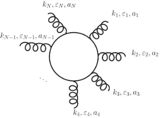
Let us start our discussion with the N-gluon vertex at the one-loop level. In standard QCD, this am-plitude can appear with a scalar, spinor or gluon in the loop. We will denote it byΓa1a2···aN
sµ1...µN[k1, . . . ,kN], s=0,12,1 indicating the spin of the loop particle. In the standard formalism, the simplest case is the one of the fermion loop, given by the single Feynman diagram in Fig. 1 and its permutations.
The off-shell vertices are not directly related to scattering amplitudes, but rather should be thought of as supplementing the tree-level (classical) gluon self-interaction vertices as loop (quantum) ver-tices. Correspondingly, their most immediate role is as input for the Schwinger-Dyson equations, the
ae-mail: [email protected]
Figure 1.Fermion loop contribution to the N-gluon vertex.
quantum generalization of the classical field equations. However, they are also important for the renor-malization group, for the infrared properties of QCD [3], for the matching of perturbative information with lattice data [4], and as building blocks for higher-loop amplitudes.
While on-shell amplitudes nowadays can, in favorable cases, be calculated explicitly at the multi-leg and/or multi-loop level, the study of these vertices is presently essentially still stuck at the one-loop four-point level. The difficulties of the off-shell case are formidable:
• The off-shell amplitudes depend on many independent Lorentz invariantski·kj,ki·εj, εi·εj. • Off-shell one-loop tensor integrals lead, beyond the two-point case, already to two-variable
hyper-geometric functions (Appell functions) [5–7]. Thus most studies of the vertices have focused not on their explicit calculation, but on the less ambitious task of finding suitable form factor (tensor) decompositions.
• They obey Ward identities that are inhomogeneous, and map theN - point to the N −1 - point vertex:
kµ1
1 Γas1µa12...µ···aNN[k1, . . . ,kN] = −igfa1a2cΓcasµ32a...µ4···NaN[k1+k2,k3,· · ·,kN]
−igfa1a3cΓ
a2ca4···aN
sµ2...µN [k1,k2+k3,· · ·,kN]
−. . . .
(+possible ghost terms)
where the fabc are the structure constants. This mixing of amplitudes with different numbers of
gluons is a direct consequence of the nonlinearity of the non-abelian field strength tensor
Fµν ≡FµνaTa=(∂µAaν−∂νAµ)a Ta+ig[AbµTb,AcνTc]. (1)
Figure 1.Fermion loop contribution to the N-gluon vertex.
quantum generalization of the classical field equations. However, they are also important for the renor-malization group, for the infrared properties of QCD [3], for the matching of perturbative information with lattice data [4], and as building blocks for higher-loop amplitudes.
While on-shell amplitudes nowadays can, in favorable cases, be calculated explicitly at the multi-leg and/or multi-loop level, the study of these vertices is presently essentially still stuck at the one-loop four-point level. The difficulties of the off-shell case are formidable:
• The off-shell amplitudes depend on many independent Lorentz invariantski·kj,ki·εj, εi·εj. • Off-shell one-loop tensor integrals lead, beyond the two-point case, already to two-variable
hyper-geometric functions (Appell functions) [5–7]. Thus most studies of the vertices have focused not on their explicit calculation, but on the less ambitious task of finding suitable form factor (tensor) decompositions.
• They obey Ward identities that are inhomogeneous, and map theN - point to the N −1 - point vertex:
kµ1
1 Γas1µa12...µ···aNN[k1, . . . ,kN] = −igfa1a2cΓcasµ32a...µ4···NaN[k1+k2,k3,· · ·,kN]
−igfa1a3cΓ
a2ca4···aN
sµ2...µN [k1,k2+k3,· · ·,kN]
−. . . .
(+possible ghost terms)
where the fabc are the structure constants. This mixing of amplitudes with different numbers of
gluons is a direct consequence of the nonlinearity of the non-abelian field strength tensor
Fµν ≡FµνaTa =(∂µAaν−∂νAµ)a Ta+ig[AbµTb,AcνTc]. (1)
In the gluon-loop case, in general ghost terms will also appear on the right-hand side. The appear-ance of ghosts can be avoided in two ways: (i) by the pinch technique [8, 9]) (ii) using the back-ground field method with quantum Feynman gauge. These two methods are, in fact, completely equivalent [10].
Let us shortly summarize what is known about the QCD vertices. The three-gluon vertex has been well-studied:
• In 1980, Ball and Chiu analyzed this vertex for the gluon loop in Feynman gauge, and derived for it a form factor decomposition (“Ball-Chiu vertex”) [11].
• In 1996, Davydychev, Osland and Tarasov extended this study to the gluon loop in an arbitrary covariant gauge, and also to the massless fermion loop case [12].
• The massive fermion loop was treated by Davydychev, Osland and Saks in 2001 [13].
• In 2006, Binger and Brodsky 2006 reanalyzed the fermion and gluon loop cases, using the back-ground field method for the latter. They also included the scalar loop, needed for supersymmetric extensions of QCD [10].
Only preliminary results exist for the four-gluon vertex:
• J.A. Gracey in 2014 studied this vertex at the symmetric point [14].
• In the same year, Binosi, Ibañez, and Papavassiliou 2014 provided a non-perturbative investigation of the vertex in Landau gauge [15].
• Eichmann, Fischer and Heupel in 2015 more generally studied the tensor structure of amplitudes with any four gauge bosons [16].
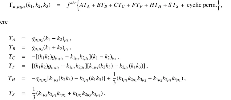
2 Ball-Chiu decomposition of the three-gluon vertex
For the three-gluon vertex, the following form factor decomposition was obtained by Ball and Chiu in 1980 [11, 17] through an explicit analysis of the Ward identity:
Γµ1µ2µ3(k1,k2,k3) = f
abcAT
A+BTB+CTC+FTF +HTH+S TS +cyclic perm.
, (2)
where
TA = gµ1µ2(k1−k2)µ3,
TB = gµ1µ2(k1+k2)µ3,
TC = −[(k1k2)gµ1µ2−k1µ2k2µ1](k1−k2)µ3,
TF = [(k1k2)gµ1µ2−k1µ2k2µ1][k1µ3(k2k3)−k2µ3(k1k3)],
TH = −gµ1µ2[k1µ3(k2k3)−k2µ3(k1k3)]+
1
3(k1µ3k2µ1k3µ2−k1µ2k2µ3k3µ1),
TS = 13(k1µ3k2µ1k3µ2+k1µ2k2µ3k3µ1). (3)
This decomposition is valid for any spin in the loop, and also for higher loop corrections. It involves six universal tensor structuresTA,TB,TC,TF,TH,TS with scalar coefficient functionsA,B,C,F,H,S. TA is just the tree-level vertex, thus at tree-level one hasA = 1 with the other coefficient functions
3 One-loop gluon amplitudes in the string-inspired formalism
A new perspective on the QCD gluon amplitudes is provided by string theory, where they appear as the infinite-string tension limit of certain string amplitudes. Along these lines, Bern and Kosower in the early nineties obtained the following “Bern-Kosower master formula” for the one-loopN- gluon amplitudes [19, 20]:
Γa1...aN[k
1, ε1;. . .;kN, εN] = (−ig)Ntr(Ta1. . .TaN)
∞
0 dT(4πT)
−D/2e−m2T
×
T
0 dτ1
τ1
0 dτ2. . . τN−2
0 dτN−1exp
N
i,j=1
1
2GBi jki·kj−iG˙Bi jεi·kj+ 1
2G¨Bi jεi·εj lin(ε
1...εN)
.
(4)
As it stands, this is a parameter integral representation for the (color-ordered)N- gluon vertex, with momenta kiand polarizations εi, induced by a scalar loop, inDdimensions. HeremandT are the
loop mass and proper-time,τithe location of theith gluon along the loop, and
GBi j=|τi−τj| −(τi−τj)
2
T ,G˙B(τi, τj)=sign(τi−τj)−2
(τi−τj)
T ,G¨B(τi, τj)=2δ(τi−τj)− 2 T .
(5)
However, in the Bern-Kosower formalism this master formula is shown to contain much more in-formation, namely it serves as a generating functional for the construction of the on-shellN- gluon amplitudes for the scalar, spinor and gluon loop. This construction proceeds through the application of the “Bern-Kosower rules”, whose content can be summarized as follows:
1. For fixed N, expand the generating exponential, keeping only the terms that are linear in each polarization vector (as indicated by the notation|lin(ε1...εN)).
2. Use suitable integrations-by-parts to remove all second derivatives ¨GBi j.
3. Apply two types of pattern-matching rules :
• The “tree replacement rules”, which generate the contributions of the missing reducible dia-grams.
• The “loop replacement rules”, which generate the integrands for the spinor and gluon loop from the one for the scalar loop.
4 Strassler’s worldline path integral approach
Shorlty after the work of Bern and Kosower, Strassler [21] rederived the master formula and the loop replacement rules using worldline path integral representations of the gluonic effective actionsΓ[A]. E.g. for the scalar loop [21–23]
Γ[A]=tr
∞
0
dT T e−
m2T
Dx(τ)Pe−0Tdτ
1
4x˙2+igx˙·A(x(τ))
5
3 One-loop gluon amplitudes in the string-inspired formalism
A new perspective on the QCD gluon amplitudes is provided by string theory, where they appear as the infinite-string tension limit of certain string amplitudes. Along these lines, Bern and Kosower in the early nineties obtained the following “Bern-Kosower master formula” for the one-loopN- gluon amplitudes [19, 20]:
Γa1...aN[k
1, ε1;. . .;kN, εN] = (−ig)Ntr(Ta1. . .TaN)
∞
0 dT(4πT)
−D/2e−m2T
×
T
0 dτ1
τ1
0 dτ2. . . τN−2
0 dτN−1exp
N
i,j=1
1
2GBi jki·kj−iG˙Bi jεi·kj+ 1
2G¨Bi jεi·εj lin(ε
1...εN)
.
(4)
As it stands, this is a parameter integral representation for the (color-ordered)N- gluon vertex, with momenta kiand polarizations εi, induced by a scalar loop, inDdimensions. HeremandT are the
loop mass and proper-time,τithe location of theith gluon along the loop, and
GBi j=|τi−τj| −(τi−τj)
2
T ,G˙B(τi, τj)=sign(τi−τj)−2
(τi−τj)
T ,G¨B(τi, τj)=2δ(τi−τj)− 2 T .
(5)
However, in the Bern-Kosower formalism this master formula is shown to contain much more in-formation, namely it serves as a generating functional for the construction of the on-shellN- gluon amplitudes for the scalar, spinor and gluon loop. This construction proceeds through the application of the “Bern-Kosower rules”, whose content can be summarized as follows:
1. For fixed N, expand the generating exponential, keeping only the terms that are linear in each polarization vector (as indicated by the notation|lin(ε1...εN)).
2. Use suitable integrations-by-parts to remove all second derivatives ¨GBi j.
3. Apply two types of pattern-matching rules :
• The “tree replacement rules”, which generate the contributions of the missing reducible dia-grams.
• The “loop replacement rules”, which generate the integrands for the spinor and gluon loop from the one for the scalar loop.
4 Strassler’s worldline path integral approach
Shorlty after the work of Bern and Kosower, Strassler [21] rederived the master formula and the loop replacement rules using worldline path integral representations of the gluonic effective actionsΓ[A]. E.g. for the scalar loop [21–23]
Γ[A]=tr
∞
0
dT T e−
m2T
Dx(τ)Pe−0Tdτ
1
4x˙2+igx˙·A(x(τ))
,
where Aµ=AaµTaandPdenotes path ordering. This rederivation made it also clear that the master formula and the loop replacement rules hold off-shell.
In [24], Strassler studied the integration-by-parts procedure in more detail, and noted that it leads to the automatic appearance of gluon field strength tensors: namely, in the bulk it rearranges polariza-tion vectors into the “abelian” part of the field strength tensor for gluoni,
fµν
i ≡k
µ
iενi −εµikiν, (6)
and it also induces color commutators [Tai,Taj] as boundary terms. Those fit together to produce full nonabelian field strength tensors (1) in the low-energy effective action. Thus we see the emergence of gauge invariant tensor structuresat the integrand level.
Strassler’s work suggests that the worldline approach may be suitable for deriving well-organized form factor decompositions for gluonic amplitudeswithout the usual tedious analysis of the Ward identities. This is indeed the case, as the present authors and V. M. Villanueva have shown in [25]. There we presented various integration-by-parts algorithms for the general N - gluon case. Two preferred representations emerged:
• The “Q- representation” usesonly local total derivative termsand relates directly to the effective action, as in [24].
• The “S - representation” usesboth local and non-local total derivative termsand is Ball-Chiu like in that all terms with trueN- point kinematics are manifestly transversal.
In [18] we then showed that theS - representation in the three-point case reproduces precisely the Ball-Chiu representation above.
5 Form-factor decomposition of the one-loop four-gluon vertex
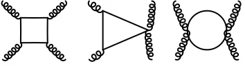
In the four-gluon case, a priori one can construct 138 tensors! It is thus surprising, that our integration-by-parts algorithms results, in both theQandS - representation, in a decomposition in terms of only 19 tensors [26, 27]. And of those, only 14 have true four-point kinematics, four tensors have pinched three-point kinematics, and one structure has doubly-pinched two-point kinematics (see Fig. 2),
(1) Figure 2.Unpinched, pinched and double-pinched diagrams.
T4
P = tr (f1f2f3f4),
T4
NP = tr (f1f3f2f4),
T22
P =
1
4tr (f1f2)tr (f3f4), T22
NP = 14tr (f1f3)tr (f2f4),
T3
P = tr (f1f2f3)ε4·k1,
T3
NP = tr (f1f2f3)ε4·k2,
Tquart2ad j = 1
2tr (f1f2)ε3·k1ε4·k1, TP2ad j = 1
2tr (f1f2)ε3·k2ε4·k1, TNP2ad j = 1
2tr (f1f2)ε3·k1ε4·k2, TC2ad j = 1
2tr (f1f2)
ε3·k4ε4·k1−12ε3·ε4k4·k1
,
TZ2ad j = 1 2tr (f1f2)
ε3·k4ε4·k2−12ε3·ε4k4·k2
,
Tquart2opp = 1
2tr (f1f3)ε2·k1ε4·k1, TP2opp = 1
2tr (f1f3)ε2·k3ε4·k1, TNP2opp = 1
2tr (f1f3)
ε2·k4ε4·k1−12ε2·ε4k4·k1
.
Note that here most, but not all, polarization vectorsεihave been absorbed into field strength tensors fi. For the corresponding tensors in theS - representation this absorption process has been completed
through the use of additional integration-by-parts steps. Those involve inverse momenta, and thus introduce spurious non-localities. “Naked” polarization vectors then appear only in the remaining five pinched tensor structures, which in the present approach arise as boundary terms in the integration-by-parts procedure. This means that the non-transversality of the amplitude, which is unavoidable, since implied by the Ward identity (1), has been pushed into the terms with a less-than-maximally complicated dependence on the external momenta. This is analogous to what one has for the Ball-Chiu vertex, and should constitute a certain advantage for the use of the vertex in the Schwinger-Dyson equations.
6 Explicit one-loop results
Let us give here also the coefficient functions of these fourteen tensors resulting from our method for the case of the scalar loop. Here we find it convenient to transform from the proper-time variables τ1, . . . , τ4to standard Feynman-Schwinger parametersα1, . . . , α4via
Tα1=1−τ1,Tα2 =τ1−τ2,Tα3=τ2−τ3,Tα4=τ3. (7)
T4
P = tr (f1f2f3f4),
T4
NP = tr (f1f3f2f4),
T22
P =
1
4tr (f1f2)tr (f3f4), T22
NP = 14tr (f1f3)tr (f2f4),
T3
P = tr (f1f2f3)ε4·k1,
T3
NP = tr (f1f2f3)ε4·k2,
Tquart2ad j = 1
2tr (f1f2)ε3·k1ε4·k1, TP2ad j = 1
2tr (f1f2)ε3·k2ε4·k1, TNP2ad j = 1
2tr (f1f2)ε3·k1ε4·k2, TC2ad j = 1
2tr (f1f2)
ε3·k4ε4·k1−12ε3·ε4k4·k1
,
TZ2ad j = 1 2tr (f1f2)
ε3·k4ε4·k2−12ε3·ε4k4·k2
,
Tquart2opp = 1
2tr (f1f3)ε2·k1ε4·k1, TP2opp = 1
2tr (f1f3)ε2·k3ε4·k1, TNP2opp = 1
2tr (f1f3)
ε2·k4ε4·k1−12ε2·ε4k4·k1
.
Note that here most, but not all, polarization vectorsεihave been absorbed into field strength tensors fi. For the corresponding tensors in theS - representation this absorption process has been completed
through the use of additional integration-by-parts steps. Those involve inverse momenta, and thus introduce spurious non-localities. “Naked” polarization vectors then appear only in the remaining five pinched tensor structures, which in the present approach arise as boundary terms in the integration-by-parts procedure. This means that the non-transversality of the amplitude, which is unavoidable, since implied by the Ward identity (1), has been pushed into the terms with a less-than-maximally complicated dependence on the external momenta. This is analogous to what one has for the Ball-Chiu vertex, and should constitute a certain advantage for the use of the vertex in the Schwinger-Dyson equations.
6 Explicit one-loop results
Let us give here also the coefficient functions of these fourteen tensors resulting from our method for the case of the scalar loop. Here we find it convenient to transform from the proper-time variables τ1, . . . , τ4to standard Feynman-Schwinger parametersα1, . . . , α4via
Tα1=1−τ1,Tα2=τ1−τ2,Tα3=τ2−τ3,Tα4=τ3. (7)
The “unpinched part” of the scalar loop amplitude then takes the following form:
Γa1a2a3a4,u
0,l =
g4 (4π)D2
tr (Ta1Ta2Ta3Ta4)Γ4−D
2 Tu l 1 0 4
i=1
dαiδ1−
4
i=1 αi
Pu
0,l
Den4−D
2
.
Here
Den≡m2+α
1α2k21+α2α3k22+α3α4k23+α1α4k24+α1α3(k1+k2)2+α2α4(k1+k3)2,
is the standard four-point off-shell denominator polynomial, and below we list the numerator polyno-mials:
P4
0,P = (1−2α1)(1−2α2)(1−2α3)(1−2α4),
P4
0,NP = −(1−2α1)(1−2α3)(1−2α2−2α3)(1−2α3−2α4),
P22
0,P = (1−2α2)2(1−2α4)2,
P22
0,NP = (1−2α2−2α3)2(1−2α3−2α4)2,
P3
0,P = −(1−2α1)(1−2α2)(1−2α3)(1−2α2−2α3),
P3
0,NP = (1−2α2)(1−2α3)(1−2α2−2α3)(1−2α3−2α4), P20ad j,quart = (1−2α1)(1−2α2−2α3)(1−2α2)2,
P20ad j,P = (1−2α1)(1−2α3)(1−2α2)2,
P20ad j,NP = −(1−2α2−2α3)(1−2α3−2α4)(1−2α2)2,
P20ad j,C = −(1−2α1)(1−2α4)(1−2α2)2,
P20ad j,Z = (1−2α4)(1−2α3−2α4)(1−2α2)2,
P20opp,quart = (1−2α2)(1−2α1)(1−2α2−2α3)2,
P20opp,P = −(1−2α1)(1−2α3)(1−2α2−2α3)2,
P20opp,NP = −(1−2α1)(1−2α3−2α4)(1−2α2−2α3)2.
(8)
7 Replacement rules, spin unification, and gauge fixing
In standard field theory, the calculation of the scalar, spinor and gluon loop amplitudes are essentially independent, and there is also no obvious way of combining the resulting structures, as would be often desirable, for example, to take advantage of cancellations implied by space-time supersymmetry in supersymmetric extensions of QCD.
˙
GBi1i2G˙Bi2i3· · ·G˙Bini1→G˙Bi1i2G˙Bi2i3· · ·G˙Bini1−GFi1i2GFi2i3· · ·GFini1 (9)
whereGFi j≡sign(τi−τj). This applies to both the Q and the S representation.
The corresponding “cycle replacement rule” for passing from the scalar to the gluon loop vertex is similar, though slightly more complicated [21, 28]. Here, however, it is important to remember that, unlike the fermion loop, for the gluon loop the vertices are gauge-dependent, and the application of the cycle replacement rule fixes the gauge in a way that, in field theory terms, corresponds to the background field method with quantum Feynman gauge. As was already mentioned above, this is the only gauge fixing that makes the gluon-loop contribution to theN- gluon vertex fulfill the same Ward identity as the scalar and fermion-loop ones. This version of the vertex is also the same one that is produced by the pinch technique.
8 Comparison with the low-energy effective action
The low energy expansion of the one-loop QCD effective action induced by a loop particle of massm can be written as
Γ[F]=
∞
0
dT T
e−m2T
(4πT)D/2 tr
dx0
∞
n=2 (−T)n
n! On[F],
whereOn(F) is a Lorentz and gauge invariant expression of mass dimension 2n. To lowest orders and
for the scalar loop, one has [29, 30]
O2 = −1
6g2FµνFµν, O3 = −152 ig3FκλFλµFµκ−
1
20g2DλFµνDλFµν, O4 = +2
35g4FκλFλκFµνFνµ+ 4
35g4FκλFλµFκνFνµ− 1
21g4FκλFλµFµνFνκ− 8
105ig3FκλDλFµνDκFνµ
−356 ig3F
κλDµFλνDµFνκ+ 11
420g4FκλFµνFλκFνµ+ 1
70g2DκDλFµνDλDκFνµ. (10)
We have matched the low-energy limit of our results for the three and four-gluon amplitudes against this effective action, and found complete agreement [27]. Apart from providing a useful check on our calculation, this also showed that our amplitude decomposition is in a one-to-one correspondence with the structures appearing in the low-energy effective action up to the four-point level. This also dispels any possible doubts that one may have had concerning the completeness of our decomposition; a priori, it would seem difficult to exclude that some structures might appear in the four-gluon vertex at higher loop orders that are not there yet at the one-loop level. However, the structure of the low-energy expansion of the effective action is known to be independent of the loop order, as well as of spin; only the numerical coefficients in this expansion will change when one goes to higher orders in perturbation theory. Therefore the fact that our 19 structures are sufficient to completely capture this expansion up to the four-gluon level at one-loop is sufficient to show that no additional tensor structures will be needed at higher loops.
9 Summary and Outlook
Let us summarize our results on the form factor decomposition of the QCD gluon vertices that we have reported here, based on [18, 25–27]:
• The worldline formalism makes it possible to generate well-organized form factor decompositions of theN- gluon vertex without the need to analyze the Ward identities.
• At the one-loop level, it allows one to unify the scalar, spinor and gluon loop contributions to theN - gluon vertex.
• We have carried out this program explicitly for the three- and four-point cases. For the three-gluon vertex, we have rederived the well-known Ball-Chiu decomposition. For the four-gluon vertex, we have obtained a Ball-Chiu like decomposition, as well as a decomposition that relates directly to the QCD effective action. Both decompositions contain 19 independent tensor structures (up to permutation).
• The main limitation of our method is that we presently do not know (yet) how to treat the gluon loop in any gauge other than background-field quantum Feynman gauge. In particular, for the use of our form factor decompositions in the Schwinger-Dyson equations it would be very desirable to generalize the gluon loop contribution to Landau gauge.
• There is also possible room for improvement in the color degree of freedom. Instead of its imple-mentation by explicit color factorsTa, as we do, one might want to follow the example of the spin
degree of freedom, and replace the color matrices by auxiliary worldline color fields. See the talk by James P. Edwards in this conference for recent progress along these lines [31–33].
• Finally, let us mention also that, in the abelian case, our tensor decompositions degenerate to only 6 instead of 19 tensors. We are presently applying this abelian decomposition to a first calculation of the QED one-loop four-photon amplitudes with all photon legs off-shell.
References
[1] H. Elvang and Y.-t. Huang, arXiv:1308.1697 [hep-th]. [2] L. J. Dixon, SLAC-PUB-15775, arXiv:1310.5353 [hep-ph].
[3] R. Alkofer, M. Q. Huber and K. Schwenzer, Eur. Phys. J. C62 (2009) 761, arXiv:0812.4045 [hep-ph].
[4] M. Pelaez, M. Tissier and N. Wschebor, Phys.Rev. D88(2013) 125003, arXiv:1310.2594 [hep-th].
[5] A. I. Davydychev and R. Delbourgo, J. Math. Phys.39(1998) 4299. arXiv: hep-th/9709216. [6] J. Fleischer, F. Jegerlehner and O.V. Tarasov, Nucl. Phys. B 566 (2000) 423, arXiv:
hep-ph/9907327.
[7] J. Fleischer, F. Jegerlehner and O.V. Tarasov, Nucl. Phys. B 672 (2003) 303, arXiv: hep-ph/0307113.
[8] J. M. Cornwall and J. Papavassiliou, Phys. Rev. D40(1989) 3474. [9] J. Papavassiliou, Phys. Rev. D47(1993) 4728.
[10] M. Binger and S. J. Brodsky, Phys. Rev. D74(2006) 054016, hep-ph/0602199. [11] J. S. Ball and T. W. Chiu, Phys. Rev. D22(1980) 2250, Erratum ibido23(1981) 3085.
[12] A. I. Davydychev, P. Osland and O. V. Tarasov, Phys. Rev. D54, 4087 (1996), hep-ph/9605348; Erratum-ibido59, 109901 (1999).
[14] J. A. Gracey, Phys. Rev. D84085011 (2011), arXiv:1108.4806 [hep-ph].
[15] D. Binosi, D. Ibañez, J. Papavassiliou, JHEP059,1409 (2014), arXiv:1407.3677 [hep-ph]. [16] G. Eichmann, C. Fischer and W. Heupel, Phys. Rev.D 92, 056006 (2015), arXiv: 1505.06336
[hep-ph].
[17] J. S. Ball and T. W. Chiu, Phys. Rev. D22, 2542 (1980).
[18] N. Ahmadiniaz and C. Schubert, Nucl. Phys. B869(2013) 417, arXiv:1210.2331 [hep-ph]. [19] Z. Bern and D. A. Kosower, Nucl. Phys. B362(1991) 389.
[20] Z. Bern and D. A. Kosower, Nucl. Phys. B379(1992) 451. [21] M. J. Strassler, Nucl. Phys. B385(1992) 145, hep-ph/9205205. [22] R.P. Feynman, Phys. Rev.80(1950) 440.
[23] C. Schubert, Phys. Rept.355(2001) 73, arXiv:hep-th/0101036.
[24] M. J. Strassler, “Field theory without Feynman diagrams: a demonstration using actions induced by heavy particles”, SLAC-PUB-5978 (1992) (unpublished).
[25] N. Ahmadiniaz, C. Schubert and V.M. Villanueva, JHEP1301(2013) 312, arXiv:1211.1821 [hep-th].
[26] N. Ahmadiniaz and C. Schubert, Int. J. Mod. Phys. E25(2016) 1642004.
[27] N. Ahmadiniaz and C. Schubert, “String-inspired form factor decompositions of the four-gluon vertex”, in preparation.
[28] M. Reuter, M. G. Schmidt and C. Schubert, Ann. Phys. (N.Y.)259(1997) 313, hep-th/9610191. [29] A. van de Ven, Nucl. Phys.B 250(1985) 593.
[30] D. Fliegner, P. Haberl, M.G. Schmidt and C. Schubert, Ann. Phys. (N.Y.)264(1998) 51, hep-th/9707189.
[31] N. Ahmadiniaz, F. Bastianelli and O. Corradini, Phys. Rev. D93(2016) 025035, Addendum: Phys. Rev. D93(2016) 049904, arXiv:1508.05144 [hep-th].