Formulation of Model Defects Suitable for the Resonance
Regime
BenediktRaab1,∗,ThomasSrdinko1,∗∗, andHelmutLeeb1,∗∗∗
1Atominstitut, TU Wien, Wiedner Hauptstrasse 8-10, 1040 Vienna, Austria
Abstract. A method to account for model deficiencies in nuclear data eval-uations in the resonance regime is proposed. The method follows the ideas of Schnabel and coworkers and relies on Gaussian processes with a novel problem-adapted ansatz for the covariance matrix of model uncertainties extending the formalism to the energy region of resonances. The method was used to evaluate a set of schematic but realistic neutron reaction data generated by an R-matrix code and a well defined model defect. Using the extended ansatz for model de-fects the Bayesian evaluation successfully recovered the built-in model defect in size and structure thus demonstrating the applicability of the method.
1 Introduction
The availability of reliable evaluated nuclear data is an important prerequisite for develop-ments in several fields of science and technology. At present, Bayesian evaluation techniques are considered as the proper tool to consistently combine experimental data with model in-formation. Because of the complexity of nuclear systems, nuclear models can only describe certain properties of the system, but not the complete system. Consequently there exist al-ways model defects and they have an important impact on evaluations [1, 2]. Several attempts for their inclusion were proposed in the past [3, 4]. Recently Schnabel [1] presented a statisti-cally consistent formulation in terms of Gaussian processes, which was applicable for smooth energy dependence of reaction cross sections and more recently for angle differential cross sections [5].
In this contribution we propose an extension of the formalism of model defects for the resonance regime, especially suited for light nuclear systems. The essential step, presented in Sect. 2, is the formulation of a new ansatz for the covariance matrix of the model defects and its inclusion in the evaluation process. In Sect. 3 the schematic example, the details of the evaluation procedure and the results are presented and discussed. The work is summarized in Sect. 4 and an outlook is given.
2 Evaluation including Model Defects
2.1 Concept of Formalism
The mathematical basis of up-to-date evaluation techniques is provided by Bayes theorem
π
~p|~σexp= 1
R
ddp l~σ exp|~p
π ~p l
~σexp|~p
π ~p. (1)
Thereby thea-priori distributionπ ~pof model parameters~
pis updated with experimental information represented by the likelihood functionl~σexp|~p
, where ~σexp is the vector of
experimental data points. The fraction in Eq. (1) acts as normalization. The result is an a-posteriori distributionπ~p|~σexpof model parameters taking into account the experiments.
In standard Bayesian evaluations it is assumed that the model is perfect, i.e.
~σexp=~σmod+~∈exp, where ~σmodand~∈exp are the vectors of model values and experimental
errors, respectively. In general model defects always occur and their neglect affects the eval-uation [1, 2]. At present it is well established that model defects must be taken into account in nuclear data evaluation. There have been several attempts to account for model defects. Recently Schnabel [1, 5] developed a statistically well defined approach based on Gaussian processes. The evaluation starts from the ansatz
~σexp=~σmod+~∈mod+~∈exp, (2)
where~∈mod is the model defect. All quantities are assumed to be random variables. For simplicity we assume multivariate normal distributions, i.e.
~σmod∼ N(~σ0,A0), ~∈mod∼ N(~0,K0), ~∈exp∼ N(~0,B), (3)
where the first argument refers to the mean value and the second one to the associated covari-ance matrix. In addition we assume that~σmod,~∈modand~∈expare mutually independent.
2.2 Model defects for the Resonance Regime
The inclusion of model defects via a Gaussian process assumes a vanishinga-priori mean value of~∈modand ana-priori covariance matrixK0which must be chosen according to the
ex-pectation. The covariance function for angle-integrated and angle-differential cross sections introduced in [1] and [5], respectively, is not suited for the resonance region. Frequently phenomenological R-matrix descriptions of the resonant part are considered to be perfect. However, the achievable description depends on several quantities which are chosen prior to a fit, i.e. the chosen matching radii, the number of poles, the choice of background poles etc. Of course one can consider these quantities as parameters of the fit, but high correla-tions and the strong non-linear relation to the observables will hamper reliable estimates of their uncertainties. Therefore a treatment as model defects of a specifically chosen model is preferable.
In order to account for model defects of the cross sectionσ(E) in the resonance regime we propose for model defects the following covariance matrix,
K0(Ei,Ej)=σ(Ei)σ(Ej)δ21·exp − 1 2λ2
1
Ei−Ej 2
+δ2 2·α
dσ dE(Ei)·α
dσ
dE(Ej)·exp
− 1 2λ2
2
Ei−Ej 2
The first term is equivalent to the expression introduced by Schnabel [1] for smooth cross sections, while the second one is sensitive to energy regions with strongly varying cross sections. The quantityαcan be considered as mean widths of the resonances,λ2as correlation
length between the resonances andδ2as a relative uncertainty with respect to the resonance
height. Usually relative high values are chosen forδ2 because a slight change in the peak
position implies a great change in the magnitude of the cross section.
2.3 Implementation of Formalism
In principle a Bayesian evaluation can be performed either by Monte Carlo techniques or in case of normal distribution by Generalized least Square (GLS) method. In this contribution we restrict ourselves to multivariate normal distributions and make use of the modified GLS-technique [1]. Thus we obtain expressions for the Bayesian update of the mean model cross sections~σ1, the mean model error~∈modand the associated covariance matricesA1andK1,
~σ1 = ~σ0+A0ST
SA0ST+SK0ST+B −1
~σexp−S~σM
, (5)
~
∈1 = K0ST
SA0ST+SK0ST +B −1
~σexp−S~σM
, (6)
A1 = A0−A0ST
SA0ST+SK0ST+B −1
SA0, (7)
K1 = K0−K0ST
SA0ST+SK0ST+B −1
SK0. (8)
where the matrixSprovides the transformation from the model grid to the experimental grid. For simplicity we assumed in Eqs. (5) to (8) that the model grid contains all energies for which experimental data are given.
Due to the ansatz (2) the evaluated cross section is not ~σ1 but~σtrue = ~σ1+~∈1 and the
corresponding covariance matrix
U1=U0−C0
SA0ST +SK0ST+B −1
CT0, (9)
withU0=SA0ST+K0andC0=A0ST+K0ST.
3 Application
In order to demonstrate the applicability of this formalism in the resonance range we apply the procedure on a schematic set of experimental data with known model defects. The example and the obtained results are discussed in detail in the following subsections.
3.1 Generation of schematic example
We start from a schematic R-matrix example of neutron-168 O scattering including all partial waves up toJ =5/2. In three partial waves, i.e. Jπ =1/2+,3/2+and 5/2−, we assume the existence of one pole leading to the single-channel R-matrix
RJπ(E)= γ
2 i
Ei−E
for Jπ=1/2+,3/2+and 5/2+ (10)
and vanishing in all other partial waves. The chosen pole energies and widths are given in Tab 1. Using the R-matrix method the cross sectionσcalc was determined for the energies
Table 1.Comparison of the originally chosen pole parameters of the R-matrix calculation (left) and the parameter values obtained by fit of the experimental data distorted by model defects.
chosen pole values fitted pole values Jπ i Ei[MeV] γi[MeV] Ei[MeV] γi[MeV]
1/2+ 1 0.70 0.20 0.685905 0.195017
3/2+ 2 1.20 0.40 1.150608 0.407358
5/2− 3 2.00 0.30 1.911950 0.355688
In order to simulate the model defect we determine the mean value of the experimental data by applying a distortion function
¯
σexp(E)= "
1+αd
dσcalc
dE (E)
#
σcalc(E) (11)
withαd =7×10⁻⁶MeV/mbarn. Choosing a subset {E1,E2,. . .,EM} of theNmesh points
we generate a set of schematic experimental data with a statistical uncertainty∈S=0.03 and a normalisation error of∈N=0.03 by
σexp(Ej)=(1+∈N) ¯σexp(Ej)· N(1,∈2S), (12)
whereN(1, S2) refers to a normal distribution with mean value 1 and the standard deviation
S. Thus we are able to construct the experimental vector~σexpwhich is of dimensionMand
theM×Mcovariance matrixBof experimental cross sections,
B=
( ¯σexp1 )2[s2+N2] σ¯exp1 σ¯exp2 N2 · · · σ¯exp1 σ¯expM N2 ¯
σexp 2 σ¯
exp
1
2 N ( ¯σ
exp 2 )
2[2 s +
2
N] · · · σ¯ exp 2 σ¯
exp M 2 N .. . · · · ... ... ¯ σexp M σ¯
exp
1
2
N σ¯
exp L σ¯
exp
2
2
N · · · ( ¯σ exp M )
2[2 S + 2 N] , (13)
where ¯σexpj =σ¯exp(Ej) .
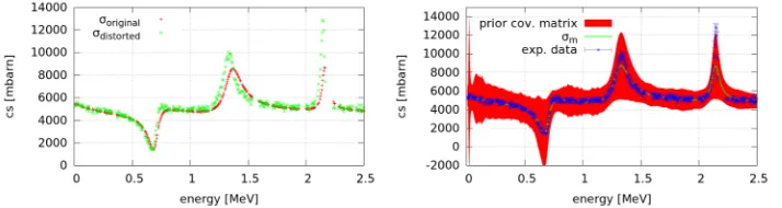
In Fig. 1 a comparison ofσcalcandσexpatMmesh points is given.
Figure 1. Left: Comparison of original and distorted data withαd = 7×10⁻⁶. Right: schematic experimental data and best parameter cross sectionσM(E) witha-priori variance p
A0(Ej,Ej) .
3.2 Generation of prior
with the R-matrix method. The best set of resonance parameters obtained from the schematic experimental data is given in Tab. 1 and yields the cross sectionσM(E) displayed in the right
part of Fig. 1.
In the next step, we assume an uncertainty width of 50% for each of the 6 best resonance parameters and performn = 200 calculations of the cross sections at all mesh points with different randomly chosen combinations of resonance parameters. Following [6] we are thus able to generate thea-priori covariance matrixA0 from the nMonte Carlo sweeps. Using
σM(E) and the parameter valuesδ1 = 0.05,λ1 = 0.5 MeV,δ2 = 1.50,α = 0.2 MeV and
λ2=0.10 MeV in Eq. (4) yields thea-priori covariance matrixK0of the model defect∈mod.
3.3 Bayesian update and results
In the previous subsection we described the generation of the schematic experimental data as well as the determination of the requireda-priori information. Thus we are able to apply the Bayesian update procedure outlined in Subsect. 2.3. At this point it should be remarked that we use a surrogate model which means that we calculate our observables~σMby the R-matrix
method on theNenergies of the evaluation mesh and use these observables as parameters of the model. Hence, every point on the mesh is a random variable, but cannot be arbitrarily varied because the properties of the model enter via thea-priori covariance matrixA0.
The only quantity we still need for the evaluation is the matrixSwhich transforms from the grid of the evaluation to the grid of energies where experimental data are given. The matrix is of dimensionM×Nand is particularly simple in our example, i.e. it has only non-vanishing elements (Si j =1) on energy points where both calculated and experimental data
are available.
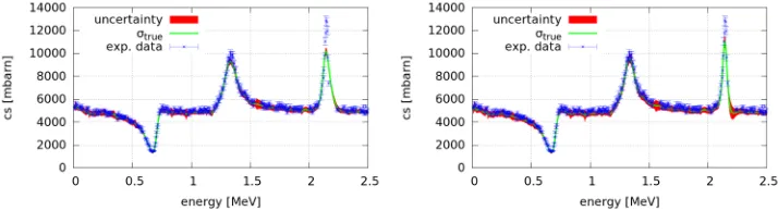
With this preparation the Bayesian evaluation of the set of schematic experimental data is straightforward and allows us to study the differences due to the inclusion of model defects. A comparison of the evaluation without and with inclusion of model defects is shown in Fig. 2. The evaluation without model defects reproduces the experimental data quite well in regions of smooth energy dependence. However, the evaluation becomes problematic at resonances which can be best identified in the third resonance at 2.14 MeV. The model can never reach the height of the experimental peak (Fig. 3). If we account for model defects the agreement of the evaluated resonance cross sections with the experimental data (Figs. 2 and 3) significantly improves.
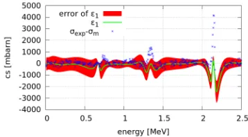
The comparison between the built-in model defect σexp -σM and the evaluated mean
model defect∈modin Fig. 4 shows a striking similarity in size and structure. This result is
very promising because it indicates that the procedure is indeed capable to extract the proper size and energy dependent structure of model defects.
(a) Without model defects (b) With model defects
Figure 3.Comparison of the third resonance, evaluated without (left) and with (right) model defects.
Figure 4.Comparison of the differenceσexp−σMwith the calculated model error∈1.
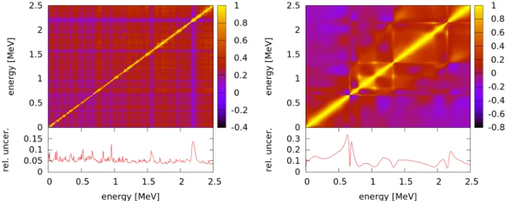
In Fig. 5 we consider the correlation matricesA1 updated without and with model
de-fects. At first glance the correlations seem to be quite similar apart from the occurrence of anticorrelations in the presence of model defects. The size of the relative uncertainties differs
(a) Without model defects (b) With model defects
significantly and confirms the general finding that uncertainties tend to be underestimated if model defects are neglected in the evaluation.
In order to complete the comparison we show in Fig. 6 the correlation matrixU1 of the
true cross sectionσtrue which is the final result which should enter in an evaluated data file.
In addition the updated covariance matrixK1of the model error∈modis also shown in Fig. 6.
Figure 6. Correlation matrices associated toU1 (left) andK1 (right) with their relative uncertainties √
U1(Ei,Ei)/σtrueand √
K1(Ei,Ei)/σtrue .
4 Summary and Outlook
We extended the recently developed formalism for model defects based on Gaussian pro-cesses [1, 5] to the resonance region. Key of the extension is the proposal of an alternative prior covariance matrixK0of model defects, Eq. (4), which is primarily sensitive to the shape
of resonances. This covariance matrix allows a Bayesian evaluation including model defects for the total energy range in a unified scheme simultaneously including the resonant and the smooth behavior of cross sections at low and intermediate projectile energies, respectively. The method also provides the magnitude of uncertainties as well as the associated covariance matrices including cross correlations between the different contributions.
References
[1] G. Schnabel,Large Scale Bayesian Nuclear Data Evaluation with Consistent Model De-fects, PhD thesis, TU Wien (2015)
[2] P. Helgesson, H. Sjöstrand, Rev. Sci. Instr.88, 115114 (2017)