Volume 8, No. 5, May – June 2017
International Journal of Advanced Research in Computer Science RESEARCH PAPER
Available Online at www.ijarcs.info
Comparative Analysis of Association Rule MiningAlgorithms in Mining Frequent
Patterns
M.Sinthuja
Department of Computer Science and Engineering Annamalai University
Chidambaram, India
Dr.N.Puviarasan
Department of Computer and Information Science Annamalai University
Chidambaram, India
Dr.P.Aruna
Department of Computer Science and Engineering Annamalai University
Chidambaram, India
Abstract: Finding frequent patterns in a huge transaction database has wide scope in research. Here in this paper we consider three of the algorithms in an association rule namely Apriori, Predictive Apriori and FP-Growth algorithm. Experiments are done to compare the result of these three algorithms with distinct datasets and present the result. Based on the results, we find that FP-Growth algorithm is more worthwhile than the Predictive Apriori and Apriori algorithms as time consumption is low and the need for candidate patterns is done away.
Keywords: Apriori; Association Rule Mining Algorithm; Datamining; FP-tree; Minimum support; Predictive Apriori; Predictive Accuracy;
Pruning
I INTRODUCTION
Data Mining came into existence in the middle of the year 1990. The volume of data is growing to a tremendous place over the last two decades due to advancement in information technology. At the same time there has been enormous development in data mining. Many methods and techniques have been added to process data and gather information. The data gathered from any source is raw data where valuable information is hidden. Here data mining is the process of obtaining the concealed useful knowledge from the huge database. Data mining is fruitful for collecting information from mammoth piles of data. In new generation, data mining has enormous applicability in software industry and other spheres due to massive quantities of data mining methods that are used in financial data analysis, Intrusion detection, scientific applications, banking, telecommunication industry etc. The main congestion in data mining is constructing quick and productive algorithms that can handle huge volumes of data.
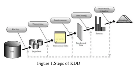
[image:1.595.44.280.659.776.2]At present, stakeholders in database research concentrate in data mining, as it is important in many spheres such as decision making, marketing strategy and in financial estimation has gained prominence. Theterm “knowledge discovery database” or KDD is used as an alternative term for data mining. Steps of KDD are shown in Fig. 1.
Figure 1.Steps of KDD
Data mining or KDD includes,
• Data cleaning: It filters the noise and inappropriate data from the database.
Data integration: It associates numerous data into individual data store.
• Data Selection: In this step we retrieve only those data which we think that is related to data mining.
• Data transformation: The data is not ready for mining even after cleaning. They need remodeling into various forms for mining. The techniques used are, aggregation, summarization etc.
• Data Mining: Here the data is accessible to apply data mining techniques to discover the interesting patterns. Techniques like classification and association analysis etc. is used for data mining.
• Pattern evaluation: This step includes visualization, transformation of patterns that are generated.
• Use of discovered knowledge: The extracted knowledge is fruitful for user to take better decision.
Among the techniques of data mining (classification, clustering, prediction and sequential pattern discovery etc.)
The most important oneis the mining association rules[7] [9].
II. ASSOCIATION RULE MINING
© 2015-19, IJARCS All Rights Reserved 1840 Association rules are regularly used in protein sequences,
market analysis, medical diagnosis, census data, CRM of credit card business etc. Many approaches have been discovered to shorten the sum of association rules, simplifying the pathway to conditions which are “intriguing” non-redundant or meeting the criteria such as coverage, leverage lift or strength.
The best way to express an association rule is by means of the expression A -> B. It means that the occurrence of item A in the database is relatively high to the occurrence of the item B. Here A is called as anterior and B is called as the subsequent. The stability of such rule can only be determined by means of its support and confidence [13] [15].
Association Rule Mining (ARM) uses the criteria of
• Support
• Confidence
Support(s) of an association rule is described as the fraction ofrecords that contains the assortment of both anterior and posterior to the overall transaction in the database collection. Support(s) is computed by the following formula:
Support (ab) = 𝑎𝑎𝑎𝑎𝑎𝑎
𝑇𝑇𝑇𝑇𝑇𝑇𝑎𝑎𝑇𝑇𝑛𝑛𝑛𝑛𝑛𝑛𝑎𝑎𝑛𝑛𝑛𝑛 𝑇𝑇𝑜𝑜𝑇𝑇𝑛𝑛𝑎𝑎𝑛𝑛𝑟𝑟𝑎𝑎𝑟𝑟𝑇𝑇𝑟𝑟𝑇𝑇𝑛𝑛 𝑟𝑟𝑛𝑛𝐷𝐷𝐷𝐷(1)
Confidence (ab) = 𝑎𝑎𝑎𝑎𝑎𝑎
𝑆𝑆𝑛𝑛𝑆𝑆𝑆𝑆𝑇𝑇𝑛𝑛𝑇𝑇(𝑎𝑎) (2)
The minimum support increases the scope of association-rule mining. However, by applying single minimum support inherently consider all items in Confidenceof an association rule.
Confidence(c) is defined as the proportion of the number of transaction that encompasses anterior and subsequent to the overall records that contain D [4] [6].
Frequent pattern mining was first introduced by Agrawal et al., in the year 1993 for Market Basket Analysis. Frequent patterns mining is an important part of association rule mining that has been active for more than 20 years still now it is very active [10].
The objective of frequent pattern mining is to find the regularly happening items in a huge database. It highlights particular patterns with supports greater than or equivalent to a minimum threshold support from bigger datasets. Pattern mining algorithm can be enforced on various data such as transaction databases etc. Frequent Patterns are itemsets, substructures that appear in a database with high frequency.
They are of
a. Candidate generation b. Pattern growth
III. VARIOUS ALGORITHMS IN ASSOCIATION RULE MINING
The following theory mainly concentrates on mining association rules of frequent patterns. ARM of Apriori algorithm, Predictive Apriori algorithm and FP-tree is adopted for the discovery of effective frequent patterns. Comparison of these algorithms shows that FP-tree is faster and efficient than Apriori and Predictive Apriori algorithm [12].
A. Apriori
The early generated algorithm of frequent patterns mining is Apriori [11] [16].As the algorithm uses prior
knowledge of frequent item set properties the algorithm is named as Apriori algorithm. Apriori apply an iterative approach known as level-wise search. This algorithm uses the method of bottom-up, breadth-first search (BFS). The concept of iteration is used to explore frequent patterns from the database [3]. It is the most favored algorithm to discover the dominant itemsets [9]. Downward closure property is applied in Apriori. The association rules are of two parameters namely support and confidence. If the support and confidence values are above user defined threshold values then the association rules are generated.
There are two steps in each iteration. The first step is the generation of set of candidate item sets. In the second step counting the occurrence of each candidate set in the database and pruning of all rules that are infrequent. The sum of database passes is equivalent to the biggest size of the regular item set. The algorithm has to perform much iteration ifthe frequent patterns are longer. As a consequence the activity of the algorithm diminishes.
For the generation of frequent patterns minsup is essential. Multiple scans are performed in Apriori. For example in the first scan counting the occurrence of item in large database i.e. candidate itemset1. If the minsup is greater than or equal to 3. The process of eliminating the patterns that are below than the minimum support is known as pruning. The candidate itemset1 minsup>=3 is eliminated by the method pruning. In the next stage tie step is executed by linking each item with the other item and searching the database for the occurrence of combination of items that are present in the database. It extends until the ultimate big itemset is discovered. Finally it explores the frequent patterns that satisfy the minimum support.
Algorithm 1: Apriori
Input: Database of Transactions D={t1, t2,…,tn Set if Items I= {I
}
1, I2…. Ik}
Frequent(Large) Itemset L Support Confidence
Method:
1. C1 = Itemsets of size one in I;
2. Determine all large itemsets of size 1, L1; 3. i = 1;
4. Repeat 5. i = i + 1;
6. Ci = Apriori-Gen(Li-1); 7. Apriori-Gen(Li-1)
8. Generate candidates of size i+1 from large itemsets of size i.
9. Join large itemsets of size i if they agree on i-1. 10. Prune candidates who have subsets that are not large. 11. Count Ci to determine Li;
The limitation of Apriori algorithm is that the algorithm has to performmore iteration if the frequent patterns are longer. As a consequence, the efficiency of algorithm decreases. It needs multiple database scrutiny andit is difficult in huge transaction database. It is not useful for real time applications.
B. Predictive Apriori Algorithm
called predictive accuracy. {Support, Confidence}=> Predictive Accuracy. This algorithm searches with an increasing support threshold for the best 'n' rules concerning a support- based corrected confidence value.
Algorithm 2: Predictive Apriori algorithm
Input: n (desired number of association rules), database with items a1. . . ak
Method:
.
1. Let τ = 1.
2. For i = 1. . .k Do: Draw a number of association rules [x⇒y] with iitems at random.
3. Measure their confidence (provided s(x) > 0). Let πi(c) be the distribution of confidences.
4. For all c,Let π(c)
∑
∏
(
𝑟𝑟
)
�𝑘𝑘𝑟𝑟�
( 2
𝑟𝑟−
1)
𝑟𝑟𝑘𝑘
𝑟𝑟=1
∑
𝑘𝑘𝑟𝑟=1�𝑘𝑘𝑟𝑟�
(2
𝑟𝑟−
1)
5. Let X0, = {∅}; Let X1 = {{a1} . . . {ak
6. For i = 1. . .k− 1 While (i = 1 or X
}} be all item sets with one single element.
i
a) If i> 1 determine the set of candidate item sets of length I as Xi = {x x’|x, x’∈X
−1 ≠∅).
i−1, |x x’| =i}.
Generation of X I can beoptimized by considering
only item sets x and x’∈Xi−1 that differ only in the
element with highest item index. Eliminate double occurrences of item sets in Xi.
b) Run a database pass and determine the support of the generated itemsets. Eliminate item sets with support less than τ from Xi.
c) For all x∈Xi Call RuleGen(x).
d) If best has been changed, Then increase τ to be the smallest number such that E (c|1,τ)
C. The FP-Growth Algorithm
To overcome the limitations of Apriori and Predictive Apriori algorithm to discover prominent patterns, the method of FP-tree was developed. FP-Growth is tree like structure [1].
The FP-tree algorithm is a novel algorithm used in mining.
The Frequent pattern tree is a modified prefix structure for
housing contained and inevitable information about FP, while the FP-growth algorithm uses the latter to find the entire set of prominent patterns. FP-growth is a divide-and-conquer algorithm that consists of two phases: build and mine [8] [16]. [5]Proved that this method exceeds other popular methods for frequent patterns mining algorithms of Apriori and Predictive Apriori Algorithm An FP-tree consists of a root node, the children of the root and a header table. Three aspect of each node are:
a. Item-name b. Count c. Node-link.
Name of the item is stored in item name. Count that stores thenumber of occurrence of an item. Node-link that points the node that contains the same item name. Each entry of Item header table consists of two characteristics:
a. Item-name b. Head of node-link
It indicates the prime node in the FP-tree having the same item-name. The items are arranged in decreasing order based on frequency of the item. FP-growth scans the database twice. The FP-growth algorithm brings about conditional pattern
base and conditional FP-tree. By using Frequent Pattern-tree frequent item sets are generated.
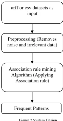
[image:3.595.356.484.113.357.2]The overall designis shown in Fig. 2.
Figure 2.System Design
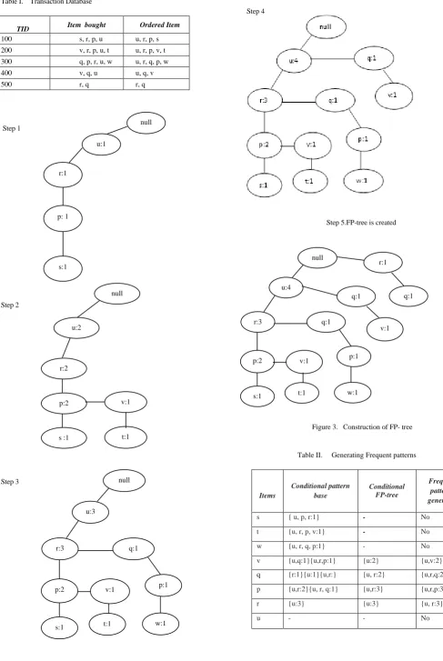
The example of FP-tree is shown inFig. 3. The transaction database is shown in the Table 1. In the Construction of FP-tree, null node is the starting point. Here the minimum support is >=2.
From the step 1, the transaction id 100 contains the itemsets of “u, r, p, s”.The first item from the tid 100 “u“ is added into the tree with count 1. The item “r“follows “u“. The items “p“and “s“are sequentially inserted. For the second transaction, the itemsets from tid 200 are “u, r, p, v, t”, for the insertion of item “u“, as null node is followed by “u“, “u“ is added to the node and the count is increased by 2. For the insertion of item “r“, node “u“ is followed by node “r“ ,the count of “r“ is incremented as 2. For the insertion of item “p“, as “r“ is followed by node “p“, the count of “p“ is incremented as 2.
In the second transaction, when the item “v“ insertion happens, a new node is created. The combination of “p“ followed by “v“ doesn't exist. Hence, a new node of “v“ is created from the node “p“. In the case of the item “t“ a new node from “v“ is created due to non-existence of the “t-v“ combination. The process is alike for the third and fourth transaction.
Likewise a node “r“ followed by “q“ is chalked out from the null node directly for fifth transaction as the “null-r“ doesn't exist. Thus the FP- tree is constructed. Table 2 shows the generation of frequent patterns.
FP growth algorithm is great in achieving three important aspirations; first one is that database is scanned only two times and computational cost is decreased dramatically. Second main objective is that candidate itemsets are not generated. Third objective is that it consequently reduces the search space by using divide and conquer approach. The limitation of FP-growth algorithm is crucial to use in incremental mining, as new transactions are added to the database, FP tree needs to be updated and the whole process needs to repeat.
arff or csv datasets as input
Preprocessing (Removes noise and irrelevant data)
Association rule mining Algorithm (Applying
Association rule)
© 2015-19, IJARCS All Rights Reserved 1842 Table I. Transaction Database
Step 1
Step 2
Step 3
Step 4
Step 5.FP-tree is created
Figure 3. Construction of FP- tree
Table II. Generating Frequent patterns
TID Item bought Ordered Item
100 s, r, p, u u, r, p, s
200 v, r, p, u, t u, r, p, v, t
300 q, p, r, u, w u, r, q, p, w
400 v, q, u u, q, v
500 r, q r, q
Items
Conditional pattern base
Conditional FP-tree
Frequent patterns generated
s { u, p, r:1} - No
t {u, r, p, v:1} - No
w {u, r, q, p:1} - No
v {u,q:1}{u,r,p:1} {u:2} {u,v:2}
q {r:1}{u:1}{u,r:} {u, r:2} {u,r,q:2}
p {u,r:2}{u, r, q:1} {u,r:3} {u,r,p:3}
r {u:3} {u:3} {u, r:3}
u - - No
null
u:1
r:1
p: 1
s:1
null
r:2
p:2 u:2
s :1
v:1
t:1
null
u:3
r:3
p:2
q:1
v:1 p:1
w:1 t:1
s:1
p:1 p:2
w:1 t:1
s:1
r:3 q:1
null
u:4
v:1
q:1
v:1 r:1
[image:4.595.296.503.62.525.2]© 2015-19, IJARCS All Rights Reserved 1843
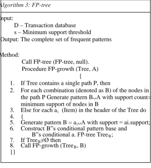
Algorithm 3: FP-tree
Input:
D – Transaction database s – Minimum support threshold
Output: The complete set of frequent patterns
Method:
Call FP-tree (FP-tree, null). Procedure FP-growth (Tree, A)
{
1. If Tree contains a single path P, then
2. For each combination (denoted as B) of the nodes in the path P Generate pattern BᴗA with support count= minimum support of nodes in B
3. Else for each ai 4. {
(Item) in the header of the Tree do
5. Generate pattern B = ai
6. Construct B‟s conditional pattern base and B‟s conditional a. FP-tree Tree
ᴗA with support = ai.support;
B; 7. If TreeB
8. Call FP-growth (Tree≠Ø then B }}
, B)
instances and 23 attributes. Training set contains 100 instance and 11attributes. KR vs KV contain 3192instance and 16 attributes
.
C. Runtime Consumption
The processing time of spect dataset for Apriori algorithm is 2seconds Predictive Apriori is 682sec and FP-growth algorithm is 1seconds. The runtime of vote dataset for Apriori algorithm is 2seconds Predictive Apriori is 140sec and FP-growth algorithm is 1seconds. The runtime of training dataset for Apriori algorithm is 0.37seconds Predictive Apriori is 18sec and FP-growth algorithm is 0.2seconds. The runtime of kv vs ks dataset for Apriori algorithm is 3seconds Predictive Apriori is 1240sec and FP-growth algorithm is 2seconds.
D. Graphical Representation of ARM algorithms for vote
dataset
[image:5.595.38.285.52.326.2]This section includes the implementation results of Association rule mining algorithms. The association rule mining algorithms of Apriori, Predictive Apriori and FP-growth are used for result analysis. The preprocessing is the first step where vote dataset is taken as input is shown in the Fig. 4.
IV. PERFORMANCE EVALUATION
A. WEKA Tool
Free and publicly available software tools for DM have been in development for the past 20 years. The goal of these tools is to facilitate the rather complicated data analysis process and to offer all interested researchers a free alternative to commercial data analysis platforms. They do so mainly by proposing integrated environments or specialized packages on top of standard programming languages, which are often open source. Open source data mining tool is particularly important and effective for small and medium enterprises (SMEs) wishing to adopt business intelligence solutions for marketing, customer service, e-business, and risk management.
WEKA is an open source data mining tool used for our analysis (www.cs.waikato.ac.nz/ml/weka/). The University of Waikato developed WEKA in New Zealand. The primary version of WEKA is no java based developed for analyzing data from the agricultural domain. WEKA is machine language. Java based version the tool is practical and used in very different applications including visualization.
To describe the data WEKA uses text files where the data files should be in the format of “.arff” and “.csv”.The attributes supported by WEKA are numeric, nominal, date, string. Even data can be read from URL or from SQL database using java database connection. The algorithms are directly applied to dataset. WEKA that includes the algorithm of classification, clustering, regression, association. It also includes visualization tools
.
B. Dataset Description
Vote and Spect dataset is used for the research and it is available in Tuned it Machine Learning Repository. Vote contains 435 instances and17 attributes. Spect contains 187
[image:5.595.307.558.337.532.2]nulll Figure 4 Preprocessing state of thevote DB(Selection of Attributes)
[image:5.595.306.558.562.747.2]© 2015-19, IJARCS All Rights Reserved 1844 During preprocessing stage noise, extraneous and
missing values were straightened out from the database. In the Fig. 5 the results of preprocessing are visualized.
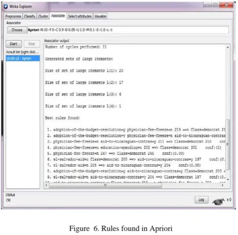
The rules generated by Apriori algorithm using original vote datasets is shown in Fig. 6.Top ten rules are generated based on support and confidence.
The rule generated by Predictive Apriori algorithm using original vote datasets is shown in Fig. 7.Rules are generated based on support and confidence.
The rule generated by FP-Growth tree using original vote datasets is shown in Fig. 8.
E. Graphical Representation of ARM algorithms for spect
dataset
[image:6.595.314.560.56.266.2]Preprocessing is performed first where spect datasets is taken as input and it is shown in Fig. 9.Here the attributes are selected based on the requirement.
[image:6.595.36.279.149.388.2]Figure 6. Rules found in Apriori
Figure 7.Rules found in Predictive Apriori
Figure 8.Rules found in FP-Growth from vote dataset
[image:6.595.313.561.337.757.2]nulll Figure 9.Preprocessing state of the spect DB
(Selection of attributes)
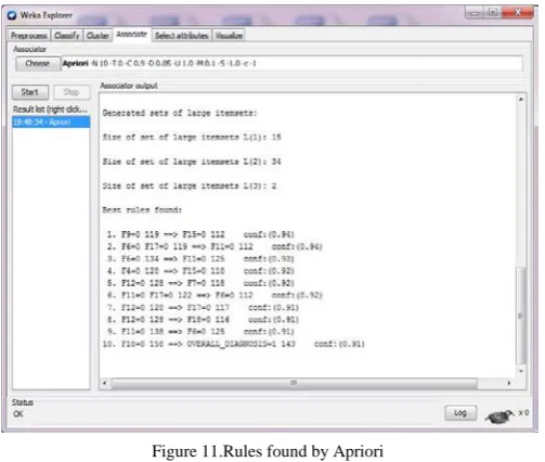
[image:6.595.32.279.448.699.2]In the Fig. 10 the results of preprocessed database is visualized after removing irrelevant data. The top ten rules generated by Apriori algorithm using spect datasets is shown in Fig. 11
.
Figure 11.Rules found by Apriori
The top rules generated by Predictive Apriori algorithm using spect datasets is shown in Fig. 12.
[image:7.595.34.286.106.319.2]Figure 12.Rules found by Predictive Apriori
Figure 13.Rules found by FP-Growth from spect dataset
The rule generated by FP-growth algorithm using spect datasets is shown in Fig. 13. Rules explored from the experiment are based on support and confidence.
Table III.Execution time of instances
Runtime of Apriori, Predictive Apriori and FP-growth algorithms for vote dataset is shown in Fig. 14.Execution time of Apriori, Predictive Apriori and FP-growth algorithms for spect dataset is shown in Fig. 15.
Figure 14. Scalability of Apriori, Predictive Apriori and FP-Growth on the basis of elapsed timefor Vote dataset
Figure 15. Execution time of Apriori, Predictive Apriori and FP-Growth for spect dataset
Apriori
FP-Growth 0
20 40 60 80 100 120 140
Vote
Ti
m
e
in
Sec
on
ds
Apriori
Predictive Apriori FP-Growth
No of Instances Execution Time in Seconds
Better
Algorithm Apriori Predictive
Apriori
FP-Growth
(Vote) 435 2 140 1
FP-Growth
(Spect) 187 2 682 1
FP-Growth
(Training set)
100 0.37 18 0.2
FP-Growth
(KR vs KV )
3192 3 1240 2
[image:7.595.324.565.118.269.2] [image:7.595.314.560.334.526.2] [image:7.595.315.560.550.743.2]© 2015-19, IJARCS All Rights Reserved 1846 Execution time of Apriori, Predictive Apriori and
FP-growth algorithms for training dataset is shown in Fig. 16.Execution time of Apriori, Predictive Apriori and FP-growth algorithms for kv vs ks dataset is shown in Fig. 17. The FP-tree is adequate and faster than Predictive Apriori and Apriori algorithm. Thus the result shows that FP-tree is superior to Predictive Apriori and Apriori algorithm. Execution time is shown in Table 3.
Figure 16. Execution time of Apriori, Predictive Apriori and FP-Growth for training dataset
Figure 17. Execution time of Apriori, Predictive Apriori and FP-Growth for
KR vs KV dataset
V.CONCLUSION
The above analysis evaluates the algorithms of Apriori, Predictive Apriori algorithm and FP-growth by the given spect, vote, training, KV vs KR dataset. The goal of Apriori, Predictive Apriori and FP-growth is to explore patterns. Based on the experimental result it shows that frequent pattern tree is superior to Apriori algorithm and Predictive Apriori algorithm. The nature of frequent pattern tree is adequate and swift than other two algorithms of Predictive Apriori and Apriori algorithm. In frequent pattern tree the need of generating candidate patterns is not required and time utilized is low. In contrast with the Apriori and Predictive Apriori algorithm, FP-growth requires scanning the database only twice. FP-growth is more adequate for bigger databases in comparison to Apriori algorithm and Predictive Apriori algorithm.
VI. REFERENCES
[1] R. Agarwal, C. Aggarwal and V. Prasad, “A tree projection algorithm for generation of frequent itemsets”. In J. Parallel and Distributed Computing, 2000.
[2] R. Agrawal, T. Imielinski and A.N.Swami, “Mining Association Rules between Sets of Items in Large Databases‟, proceedings of ACM SIGMOD Intl. Conf. Management of Data, , San Jose, CA ,vol. 22 ,pp. 207-216, 1993.
[3] R.Agrawal, R.Srikant, “Fast algorithms for mining association rules”, Proceedings of the 20th Very Large Databases Conference (VLDB‟94), Santiago de Chile, Chile, 1994.
[4] M.S. Chen, J. Han, P.S. Yu, “Data mining: an overview from a database perspective‟, IEEE Transactions on Knowledge and Data Engineering, 1996.
[5] J. Han, Pei, Y. Yin, “Mining frequent patterns without candidate generation”, Proceedings 2000 ACM-SIGMOD International Conference on Management of Data (SIGMOD‟ 00), Dallas, TX, USA, 2000.
[6] B. Liu, W. Hsu, Y. Ma, “Mining association rules with multiple minimum supports”, Proceedings of the ACM SIGKDD International Conference onKnowledge Discovery and Data Mining (KDD-99), San Diego, CA, USA, 1999.
[7] H. Mannila, “Database methods for data mining, Proceedings of the 4th International Conference on Knowledge Discovery and Data Miningtutorial‟, New York, NY, USA, 1998. [8] M. Sinthuja, N.Puviarasan and P.Aruna, “Evaluating the
Performance of Association Rule Mining Algorithms”, in World Applied SciencesJournal 35 (1): 43-53, 2017.
[9] Neelamadhab Padhy, “Dr. Pragnyaban Mishra, and Rasmita Panigrahi,The Survey of Data Mining Applications And Feature Scope”, International Journal of Computer Science, Engineering and Information Technology (IJCSEIT), Vol.2, No.3, 2012.
[10] Philippe Fournier-Viger, ”An introduction to frequent pattern
mining”,
viger.com/introduction-frequent-pattern-mining/
[11] S. Pramod,O.P.Vyas, ”Performance Evaluation of some Online Association Rule Mining Algorithms for sorted and unsorted Data sets”, International Journal of Computer Applications (0975 – 8887) Vol. 2 – No.6, 2012.
[12] M.Sinthuja, P.Aruna and N.Puviarasan, “Experimental Evaluation of Apriori and Equivalence Class Clustering and Bottom Up Lattice Traversal (Eclat) Algorithms”, Pak. J. Biotechnol. Vol. 13 special issue II pp. 77 - 82 (2016).
[13] Priyanka Asthana,Anuj Singh,Diwakar Singh, “A Survey on Association Rule Mining Using Apriori Based Algorithm and Hash Based Methods”, International Journal of Advanced Research in Computer Science and Software Engineering, Vol. 3, Issue 7, 2013.
[14] Sotiris Kotsiantis, Dimitris Kanellopoulos,“ Association Rule Mining: ARecent Overview GESTS”, Vol. 32(1), pp.71-82, 2006.
[15] T. Scheffer, ”Finding Association Rules that trade Support Optimally against Confidence. In proc. Of thye 5th
[16] M. Sinthuja, N. Puviarasan and P. Aruna, “Comparison of Candidate Itemset Generation and Non Candidate ItemsetGeneration Algorithms in Mining Frequent Patterns”, International Journal on Recent and Innovation Trends in Computing and Communication Volume: 5 Issue: 3,pp.192-197.