A Selective Analysis of Microarray Data Using Association Rule Mining

Procedia Computer Science 47 ( 2015 ) 3 – 12

1877-0509 © 2015 The Authors. Published by Elsevier B.V. This is an open access article under the CC BY-NC-ND license (http://creativecommons.org/licenses/by-nc-nd/4.0/).

Peer-review under responsibility of organizing committee of the Graph Algorithms, High Performance Implementations and Applications (ICGHIA2014) doi: 10.1016/j.procs.2015.03.177

ScienceDirect

A Selective Analysis of Microarray Data using

Association Rule Mining

Alagukumar. S

_{, Lawrance. R}

_,

a _{Research Scholar in Computer Science, Ayya Nadar Janaki Ammal College, Sivakasi – 626 124, Tamil Nadu,}

India. [email protected]

b _{Director, Department of Computer Applications, Ayya Nadar Janaki Ammal College, Sivakasi – 626 124, Tamil Nadu, India.}

[email protected]

Abstract

Association analysis plays the vital role in the computational biology. DNA Microarrays allow for the simultaneously monitor of expression levels for thousands of genes or entire genomes. Microarray gene association analysis is exposing the biological relevant association between different genes under different experimental samples. Mining association rules has been applied successfully in various types of data for determining interesting association pattern. Frequent pattern mining is becoming a potential approach in microarray gene expression analysis. In this paper the most relevant mining association rules as well as main issues when discovering efficient and practical method for microarray gene association analysis have been reviewed.

© 2015 The Authors. Published by Elsevier B.V.

Peer-review under responsibility of organizing committee of the Graph Algorithms, High Performance Implementations and Applications (ICGHIA2014).

Keywords: Data mining, Microarray gene expression data, frequent pattern mining, gene association rules, gene expression analysis;

1. Introduction

Microarray technologies provide a powerful tool by which the expression patterns of thousands of genes can be monitored simultaneously whose application range from cancer diagnosis to drug response. Gene expression is the conversion of the DNA sequences into mRNA sequences by transcription then translated into amino acid sequences called proteins.

Microarray technologies provide the opportunity to compute the expression level of tens of thousands of genes in cells simultaneously. The expression level is associated with the corresponding protein made under different conditions. Microarray experiments produced large volume of data. Microarray data presents the main challenge that is high density of data. The data collected from a microarray experiments is commonly in the form of an M x N matrix of expression level, where M represents rows and N represents column. In this study, it has been focused on Microarray gene association analysis from a © 2015 The Authors. Published by Elsevier B.V. This is an open access article under the CC BY-NC-ND license

(http://creativecommons.org/licenses/by-nc-nd/4.0/).

Peer-review under responsibility of organizing committee of the Graph Algorithms, High Performance Implementations and Applications (ICGHIA2014)

frequent pattern mining approach. Frequent pattern mining is the most important task of association rules mining methods. The residue of the paper is organized as follows. Section 2 reviewed microarray dataset, discretization and mining association rules. Section 3 reviewed the methodology of frequent pattern mining. In section 4 we compare the algorithms. In section 5 concludes this survey.

2. Methods

2.1 Data format

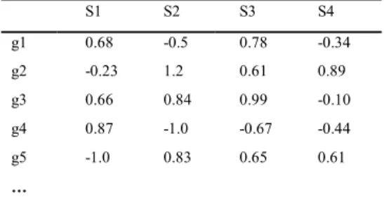
The microarray dataset can be form of an M x N matrix D of expression values, where the row represents genes g1, g2, g3…, gn and the column represents different experimental conditions (samples) s1,

s2, s3… sn. Each element D [i,j] represents the expression level of the gene gi in the sample sj (see Table 1).

The matrix usually contains large amount of data [10], therefore data mining techniques are used to extract useful knowledge.

Table 1. Microarray Dataset

S1 S2 S3 S4 g1 0.68 -0.5 0.78 -0.34 g2 -0.23 1.2 0.61 0.89 g3 0.66 0.84 0.99 -0.10 g4 0.87 -1.0 -0.67 -0.44 g5 -1.0 0.83 0.65 0.61 …

Most of the application of association rule mining on microarray gene expression still relies on discretization tasks before applying any data mining technique [2]. The normalized microarray dataset is usually represented as a series of continuous numbers [1]. Discretization is the process of transformation from continuous data into discrete data.

The threshold method used to discretize the data. This method is suitable for microarray analysis [6, 7]. Genes with log expression values greater than a particular value are considered as over expressed, otherwise as under expressed. Using threshold method each gene expression is converted into one of the two discrete values 1, 0 for over expressed and under expressed.

Threshold value is calculated by following given method, threshold value is 6.0 calculated from data matrix D [i,j]. Using threshold value, the data matrix D is converted into data matrix D’.

Table 2: Discretized Microarray data

S1 S2 S3 S4 g1 1 0 1 0 g2 0 1 1 1 g3 1 1 1 0 g4 1 0 0 0 g5 0 1 1 1

Threshold t = min((D[i,j])+max(D[i,j])-min(D[i,j]))/2

D’ [i,j] = 1 D[i,j] ≥t, (gi is over expressed at sj) 0 Otherwise, (gi is under expressed at sj)

Therefore, in order to mining association rules, microarray data matrix D is converted into matrix D’

(as shown in Table2) depending on the particular threshold value t. The microarray gene expression is converted into 1, 0 if it is ≥6.0 the expression converted into 1 otherwise 0.

2.3 Mining Association Rules

Association rules are an important class of methods of finding patterns in data. Mining association rules technique extract interesting relationships among set of items (genes) in large amount of data.

One of the most famous applications of these techniques is market basket analysis [3,4] where the main objective is to find relationships between the purchased items under different transaction. An association rule is applied on microarray dataset in order to find the relationships between genes under different samples. The association rule definition proposed by [4] is presented.

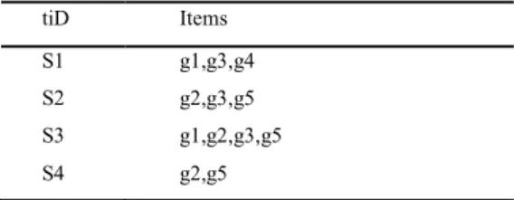
Table 3: Microarray Transaction (samples) Dataset

tiD Items S1 g1,g3,g4 S2 g2,g3,g5 S3 g1,g2,g3,g5 S4 g2,g5

Definition 1 (Association Rule) Let I = {i1, i2, i3 … im} be a set of m elements called items. A rule is defined as an implication of the form X→Y, where X, Y I and X ∩ Y = Φ. The left-hand side of the rule is named as antecedent and right-side of the rule is named as consequent. Mining Association rules technique is applied to microarray dataset to discovering interesting relationships among set of genes.

For example, an association rules between genes in the form of gene1→gene2, gene3 which means

gene1 is over expressed it is also very likely to observe an over expression of gene2 and gene3.

Definition 2 (Transaction)Let T = {t1, t2, t3 … tn} be a set of n subsets of items called transaction. Each

transaction in T identifies a subset of items [3].

Definition 3 (Support of item set) The support of an item set X, support(X), is defined as the number of transaction in T which contain the item set X [3].

Support(X) = {t א |T|X ك t}

Definition 4 (Frequent item set) Given a set of items I= {i1, i2, i3… in} and a set of transaction T = {t1, t2, t3 … tm}, a subset of I, SكI,is called a frequent if support(S) ≥ minimum support, where minimum support is a user defined threshold [3].

Definition 5 (Support of rule)The rule X→Y holds in the transaction set T with support s, where s is the percentage of transactions in T that contain X ׫ Y[3].

Support (X ׫ Y) Support (X→Y) =

|T|

Definition 6 (Confident of rule)The rule X→Y has confidence c in the transaction set D, where c is the percentage of transactions in T containing X that also contain Y[3].

Support (X ׫ Y) Confidence (X→Y) =

Support(X)|

Definition 7 (Strong/Confident of rule) Rules that satisfy both a minimum support threshold and a minimum confident threshold are called strong/confident rules [3]. If support (X→Y) ≥ minimum support and confident (X→Y) ≥ minimum confident, the rule X→Y is called strong or confident association rules where, minimum confident is user defined threshold.

Mining confident association rule is performed in two steps [4, 5]: 1. Generate all frequent n-itemsets.

2.

are frequent n-itemsets.

3. Methodology

3.1 Apriori Algorithm Input:

D, a database of transactions;

Min_sup, the minimum support count threshold. Output:

L, frequent itemsets in D.

This method carries out a breadth-first search to enumerate each 1-itemset. Again and again, join (k-1)-item sets with itself to get a k-(k-1)-item sets=2,3,...., L; where L represents the longest-frequent (k-1)-item sets. The Apriori Algorithm [4] is an important algorithm for mining frequent itemsets. A subset of a frequent itemset must also be a frequent itemset.

It uses pruning step if there is any itemset which is infrequent, its superset should be infrequent. Iteratively find frequent itemset with cardinality from 1 to k (k-itemsets). K is the longest frequent itemsets.

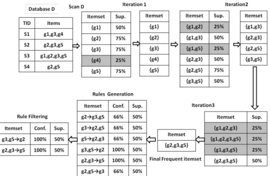
A simple Apriori instance to present a better understanding of frequent pattern mining on microarray data is explained in Figure 1. Let D be a discretized matrix (Table2). Table 3 represents the transaction and their items.

The Apriori algorithm performs a breadth-first search through the search space of all the itemsets by iteratively generating candidate itemsets. At each iteration, the support of each itemset is calculated, and pruned those itemsets with support is under the threshold. In figure 1, the removed itemsets are colored. The resulting itemsets are joined to create a new itemsets.

The algorithm ends when no new candidate group can be generated. After three iterations, the final frequent itemsets is generated. From this frequent itemset the association rules are generated. At last generated rules are filtered by some criterion. In figure1, the confidence = 100%.

Apriori based methods gives good performance with sparse dataset. The dataset such market basket data. Sparse data has the property that the number of items in the dataset is less than number of transaction. This type of data is called sparse.

Therefore, the frequent patterns are very short. However, with dense dataset such as microarray, censes data etc., Dense data has the property that the number of items (genes) in the dataset is higher than the number of transaction (Conditions). This type of data is called dense. Where there are many long frequent patterns. Dense dataset require large memory.

This drawback is due to the high exponential time cost of the generation of candidate set used by Apriori based approaches.

3.2 FP-Growth Algorithm

FP-Growth [8] allows frequent itemset discovery without candidate itemset generation. FP-growth follows divide and conquer strategy.

Growth algorithm is constructed in two steps: Step 1: Build a compact data structure called the FP-tree built using two passes over the data-set. Step 2: Extracts frequent itemsets directly from the FP-FP-tree

FP-Create Tree

Input: Database, minimum support Output: FP-Tree

Scan DB & count all frequent items. Create null root & set as current node.

For each Transaction T Sort T’s items.

For each sorted Item I

Insert I into tree as a child of current node. Connect new tree node to header list.

FP-Growth

Input: FP-Tree, f (frequent itemset) Output: All frequent patterns 3.2.1: FP-Tree Construction

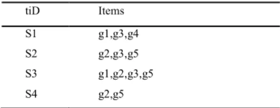
Table 4: Microarray Transaction (samples) Dataset from discretized matrix

tiD Items

S1 g1,g3,g4

S2 g2,g3,g5

S3 g1,g2,g3,g5

S4 g2,g5

FP-Tree is constructed using two passes over the data-set:

Pass 1: Scan data and find support for each itemset and remove infrequent items. Then Sort frequent items in decreasing order based on their support. In this example the minimum support count is 2.

Pass 2: FP-Growth reads one transaction at a time and maps it to a path. In FP-tree fixed order is used, so paths can overlap when transactions share items, such that when they have the same prefix. In this case, counters are incremented and link nodes are maintained between nodes containing the same item, creating singly linked lists the more paths that overlap, the higher and the compression. FP-tree may fit in memory. Frequent itemsets extracted from the FP-Tree.

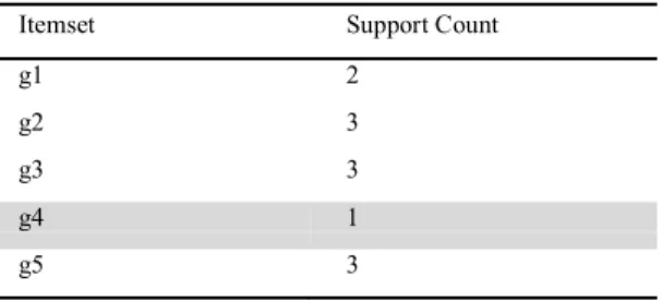
Table 5: 1 – Candidate itemset for FP-Growth

Itemset Support Count

g1 2

g2 3

g3 3

g4 1

g5 3

Generate 1-candidate itemset and arrange the items in descending order of minimum support L= {g2:3, g3:3, g5:3, g1:2}. In table 5, the removed itemsets are colored.

S1 - items in descending order <g3, g1>

S3 - items in descending order <g2, g3, g5, g1>

Complete FP-Tree

Fig: 2. Complete FP-Tree for Transaction dataset

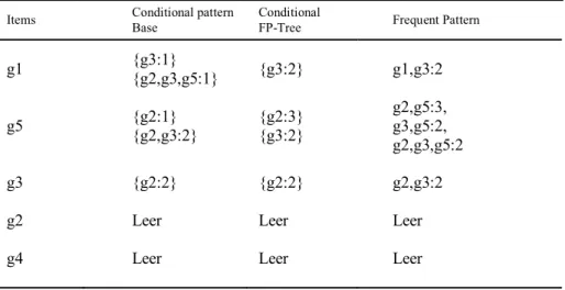
Table 6: Mining the FP-Tree by Creating Conditional Pattern Bases

Items Conditional pattern_Base Conditional_FP-Tree Frequent Pattern

g1 {g3:1}_{g2,g3,g5:1} {g3:2} g1,g3:2

g2 Leer Leer Leer

g4 Leer Leer Leer

4. Analysis of Algorithms

In this section we analysis the frequent patterns mining methods with Apriori and FP-Growth Algorithms on microarray gene expression data.

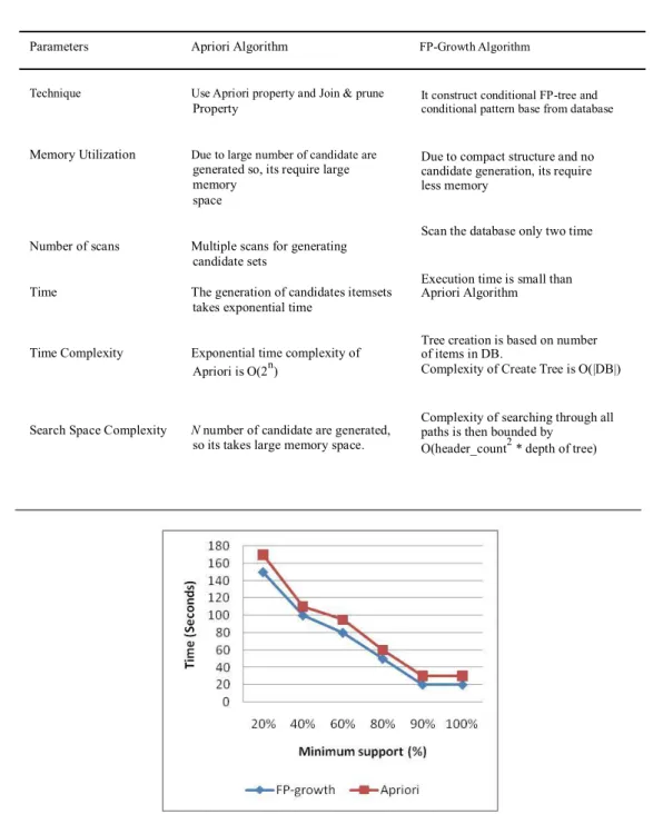
Table 7: Comparative analysis of frequent pattern mining methods using Apriori and FP-Growth algorithms on microarray gene data

Parameters Apriori Algorithm FP-Growth Algorithm

Technique Use Apriori property and Join & prune Property

Memory Utilization Due to large number of candidate are generated so, its require large memory

space

Number of scans Multiple scans for generating candidate sets

Time The generation of candidates itemsets

takes exponential time

Time Complexity Exponential time complexity of

Apriori is O(2n)

Search Space Complexity N number of candidate are generated, so its takes large memory space.

It construct conditional FP-tree and conditional pattern base from database

Due to compact structure and no candidate generation, its require less memory

Scan the database only two time

Execution time is small than Apriori Algorithm

Tree creation is based on number of items in DB.

Complexity of Create Tree is O(|DB|)

Complexity of searching through all paths is then bounded by

O(header_count2 * depth of tree)

The Apriori and FP-Growth algorithm are tested over the microarray dataset, All the datasets are publicly available and were downloaded from BRB-Array Data Archive for human cancer gene expression repository2 ( http://linus.nci.nih.gov/brb/DataArchive_New.html) [11]. It has been tested with Leukaemia dataset [9]. Fig.3 shows the running time, represented with two curves. The comparative study shows that FP-Growth is faster than Apriori algorithm.

5. Conclusion

In this paper, it has been reviewed that Apriori and FP-Growth algorithms for mining frequent pattern from microarray gene expression data. From this analysis it has been studied that interesting issues related to frequent pattern mining of the evolution of biological pattern. The microarray platforms provide dense dataset. So that, mining frequent patterns need to search efficiently for association analysis on dense data.

Like that microarray data, censes data, telecommunication data, etc., therefore, Apriori and FP-Growth algorithms are generating all frequent itemsets in such dense datasets requires large memory as well as it takes high computational time. Both Apriori and FP-Growth are aiming to find out complete set of patterns but, FP-Growth is more efficient than Apriori in respect to long patterns.

In future the algorithm will be modified to overcome both computational time and memory explosion problems for biological patterns.

References

[1] Zakaria,W., Kotb,Y., and GhalebF., “MCR-Miner: Maximal Confident Association Rules Miner Algorithm for Up/Down- Expressed Genes”, International journal of Applied Mathematics and Information Sciences, 2014, vol.8, no.2, pp.799-809. [2] Alves,R., Rodriguez-Baena,D,S, and Aguilar-Ruiz,J,S, ”Gene association analysis: a survey of frequent pattern mining from

gene expression data”, Briefings in Bioinformatics, 2009, vol.2, no.2, pp.210-224.

[3] Han,J., and Kamber,M., Data Mining: Concepts and Techniques, Morgan Kaufmann Publishers, Elsevier, 2002.

[4] Agrawal,R., Imielinski,T., Swami,A., “Mining association rules between sets of items in large databases”. In: Proceedings of the 1993 ACMSIGMOD International Conference on Management of Data. Washington, DC, USA: ACM Press, 1993; pp.207–216. [5] Agrawal,R., and Srikant,R., “Fast Algorithms for Mining Association Rules”, Proceedings of the 20th Int. Conf. on Very Large

Data Bases (VLDB94), Santiago de Chile, 1994;pp. 475-486.

[6] Wang, J., Han,J., and Pei,J., “CLOSET+ searching for the best strategies for mining frequent closed itemsets”. In: proceedings of the Ninth ACM SIGKDD International Conference on Knowledge Discovery and Data Mining. Washington, DC, USA: ACM, 2003.

[7] Agrwal,J., and Rames,J,C.,h. “Analysis of Gene Microarray Data using Association Rule Mining”, Journal of computing, 4, 2012.

[8] Han,J., Pei,J., and Yin.Y., “Mining frequent patterns without candidate Generation”, in: Proceeding of ACM SIGMOD International Conference Management of Data, 2000, pp.1-12.

[9] Antonie L, Bessonov K (2011) Classifying microarray data with association rules. In: ACM Symposium on Applied Computing. 94–99.

[10] Tuimala,J., and Laine,M.M., “DNA Microarray Data Analysis”, Second Edition, Picaset Oy, Helsinki, 2005. [11] http://linus.nci.nih.gov/brb/DataArchive_New.html