Auto Regressive based Feature Extraction and Classification of Epileptic EEG using Artificial Neural Network

Volume 4, No. 9, July-August 2013

International Journal of Advanced Research in Computer Science

RESEARCH PAPER

Available Online at www.ijarcs.info

ISSN No. 0976-5697

Auto-Regressive based Feature Extraction and Classification of Epileptic EEG using

Artificial Neural Network

Ashish Raj1, Manoj Kumar Bandil2, D B V Singh3, Dr.A.K Wadhwani4

[email protected],[email protected],[email protected],[email protected]

Abstract— Epilepsy is a neurological condition in which is due to chronic abnormal bursts of electrical discharge in the brain. Monitoring brain activity through the electroencephalogram (EEG) has become an important tool in the diagnosis of epilepsy. The EEG recordings of patients suffering from epilepsy show two categories of abnormal activity: inter-ictal, abnormal signals recorded between epileptic seizures; and ictal, the activity recorded during an epileptic seizure. The EEG signature of an inter-ictal activity is occasional transient waveforms, as isolated spikes, spike trains, sharp waves or spike-wave complexes. EEG signature of an epileptic seizure (ictal period) is composed of a continuous discharge of polymorphic waveforms of variable amplitude and frequency, spike and sharp wave complexes, rhythmic hyper synchrony, or electro cerebral inactivity observed over a duration longer than the average duration of these abnormalities during inter-ictal periods. Generally, the detection of epilepsy can be achieved by visual scanning of EEG recordings for inter-ictal and ictal activities by an experienced neurophysiologist. However, visual review of the vast amount of EEG data has serious drawbacks. Visual inspection is very time consuming and inefficient, especially in the case of long-term recordings. In addition, disagreement among the neurophysiologists on the same recording is possible due to the subjective nature of the analysis and due to the variety of inter-ictal spikes morphology. The main objective of our research is to analyze the acquired EEG signals using auto-regressive features and classify them into different classes. After feature extraction secondary goal is to improve the accuracy of classification. In order to achieve this we have applied a backpropgation based neural network classifier.100 subjects from each set were analysed for feature extraction and classification and data were divided in training, testing and validation of proposed algorithm.

Index Terms— EEG, Spike detection; Wavelet transform; Neural network, Auto-Regression, Inter-Quartile Range, Epilpepsy, Seizure

I. IINTRODUCTION

Given that ictal recordings (recording during an epileptic seizure) are rarely obtained, EEG analysis of patients suffering from epilepsy usually relies on inter-ictal findings. In those inter-ictal EEG recordings, epileptic seizures are usually activated with photo stimulation, hyperventilation and other methods [1]. However, one weakness of these Monitoring brain activity through the electroencephalogram (EEG) has become an important tool in the diagnosis of epilepsy. The EEG recordings of patients suffering from epilepsy show two categories of abnormal activity: inter-ictal, abnormal signals recorded between epileptic seizures; and ictal, the activity recorded during an epileptic seizures.

During inter-ictal periods, or between epileptic seizures, EEG recordings of patients affected by epilepsy will exhibit abnormalities like isolated spike, sharp waves and spike- wave complexes (usually all termed as inter-ictal spikes or spikes). In ictal periods, or during epileptic seizures, the EEG recording is composed of a continuous discharge of one of these abnormalities, but extended over a longer duration and typically accompanied by a clinical correlate.[2,3]

The classification of EEG signals is highly important in medical field. This can provide the knowledge of status of human mind. This helps in curing many diseases after diagnosis or classification results. So this is the important step carried out after the feature extraction for analyzing the EEG signals. There are many signal processing algorithms present for classification of features of the EEG signals. We have used SCGA (Scaled Conjugate Gradient Back Propagation Neural Network) algorithms for classification and also known as classifiers.[4]

A. Auto-Regressive Process:

The power spectral density (PSD) of the EEG signals is computed by using Burg Autoregressive (AR) Model in the present work. This method is based on minimization of forward and backward prediction errors while constraining the AR parameters to satisfy the Levinson-Durbin recursion process. Autoregressive coefficients provide us the important features in terms of the power spectral density (PSD). The Burg method estimates the reflection coefficients ak. Since,

this method describes the input signals by using the all pole model. So the selection of model order is critical because the very low model order produces smooth spectrum and too large model order effect in stability. Any stochastic process can be modeled by using AR process.[5,6,7]

Assume our samples, x (0), x (1), …, x(L-1) are drawn from an Mth-order AR model with a zero-mean IID sequence, w(n) as input is given as-

(1.1)

A corresponding difference equation is given as-

(1.2) The Magnitude Spectrum is of the form

(1.3)

(1.4)

Where f represents the model parameters and s is referred to M M

z

a

z

a

z

a

z

H

−

−

−

−

=

...

1

1

)

(

)

(

)

(

...

)

2

(

)

1

(

)

(

n

a

x

n

a

x

n

a

x

n

M

w

n

x

=

−

+

−

+

+

−

+

2 2 2 1 1 2 ... 1 ) ( M M w j z a z a z a e R − − − _{− − −} − = σ ω 2 2 2 2 2 1 1 2 _ˆ ... 1 ˆ ) ( s ft w p p w j AR z c z c z c e

R ω σ = σ

as a frequency scanning vector or steering vector. We must estimate the noise power, the model order AND the filter coefficients. This would be easy except we know that an AR model of order p > M will produce a smaller error than p = M.

II. METHODOLOGY

A. Auto-Regressive Process using Burg:

The Burg Method block estimates the power spectral density (PSD) of the input frame using the Burg method. This method fits an autoregressive (AR) model to the signal by minimizing (least squares) the forward and backward prediction errors while constraining the AR parameters to satisfy the Levinson-Durbin recursion. [10]

We can also estimate the coefficients using the iterative Burg method:

We can also estimate the coefficients using the block estimation approach:

We can convert the reflection coefficients to predictor coefficients using:

The Burg method is known to produce very high resolution spectral estimation from short data segments. However, it is sensitive to model order. It is also associated with a phenomenon known as line splitting in which a single peak in the spectrum is represented by two distinct peaks. This is often a side-effect of its tendency to underestimate the bandwidth of the poles in the signal and a tendency to favor harmonic processes.

B. Model Order Selection:

Recall that the error decreases as we increase the model order, so in most typical situations, it is difficult to determine an optimum model order.

We prefer models with lower orders following the principle of parsimony (or Occam’s razor).[8 ,9]

We could simply set an arbitrary threshold on the error, but such thresholds can vary with the application. Some common criteria (choose minimum) are:

Minimum Final Prediction Error:

tends to underestimate the model order. Akaike’s Information Criterion (AIC):

tends to overestimate the model order.

Criterion Autoregressive Transfer Function (CAT):

These approaches have not been very successful in practice.

a. Burg showed that the AR estimate is a maximum entropy estimate if the signal is Gaussian and the exact correlation values are known.

b. Burg also suggested that if the p correlation values are known, the remaining correlation values can be extrapolated in such a way to maximize the uncertainty (entropy) of the signal. We can use our autocorrelation relation:

The Burg method attempts to extrapolate these values. The maximum entropy concept represented a new way of thinking when it was first introduced. In recent years, statistical extrapolation techniques such as Bayesian methods have created a similar revolution.

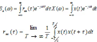
C. Calculation of Power Spectral Density:

The power spectral density (PSD) Sx (w) for a signal is a measure of its power distribution as a function of frequency. The integral of the PSD over a given frequency band computes the average power in the signal over that frequency band. Different algorithms are used for the estimation of PSD. FFT method has been widely used to analyze EEG signals yet it is not well suited to the non-stationery characteristics of the EEG signal. To overcome this limitation, the Period gram method is commonly used for computing PSD. However, the methods require averaging of several periodograms to decrease the variance of the FFT method; this averaging may in fact obscure the detection of dynamic changes in the frequency domain which are of clinical interest as in case of epileptic seizures. PSD is computed by squared modulus of the Fourier transform of the time series of the signal. [10]

Where Sx(w) is the Power Spectral Density (PSD).

The power dissipated in the range fo to fo+dfo is equal to

And Sx (.) has units Watts/Hz.

Where,

D. Calculation of Inter-Quartile Range:

In descriptive statistics, the interquartile range (IQR), also called the midspread or middle fifty, is a measure of statistical dispersion, being equal to the difference between the upper and lower quartiles. The interquartile range of a data set is the difference between the third quartile and the first quartile.

It is the range for the middle 50% of the data. It overcomes the sensitivity to extreme data values.

IQR = Q3− Q1.

(2.4) It is a trimmed estimator, defined as the 25% trimmed mid-range, and is the most significant basic robust measure of scale. It is the 3rd Quartile of a box plot plot minus the first quartile.

III. FEATUREEXTRACTION

a. Data base- The raw EEG signal is obtained from university of Bonn which consists of total 5 sets (classes) of data (SET A, SET B, SET C, SET D, and SET E) corresponding to five different pathological and normal cases. Three data sets are selected from 5 data sets in this work. These three types of data represent three classes of EEG signals (SET A contains recordings from healthy volunteers with open eyes, SET D contains recording of epilepsy patients in the epileptogenic zone during the seizure free interval, and SET E contains the recordings of epilepsy patients during epileptic seizures)

All recordings were measured using Standard Electrode placement scheme also called as International 10-20 system. Each data set contains the 100 single channel recordings. The length of each single channel recording was of 26.3 sec.The 128 channel ampli fier had been used for each channel [11]. The data were sampled at a rate of 173.61 samples per second using the 12 bit ADC. So the total samples present in single channel recording are nearly equal to 4097 samples (173.61×23.6). The band pass filter was fixed at 0.53-40 Hz (12dB/octave) [12].

Autoregressive (AR) coefficients describe the important features of EEG signals, the correct choice of model order is important. Too low and too high order gives the poor estimation of power spectral density (PSD) . In the present work, Burg’s method is used for calculating the AR coefficients.The model order of 10th is set to the input signals by minimizing the forward and backward prediction errors for the AR parameters to satisfy the Levinson-Durbin recursion.The plot of AR coefficnts for the three datasets are shown below-

Figure 3.1 Plot of AR Coefficients of Set-F

Figure 3.2 Plot of AR Coefficients of Set-S

Figure 3.3 Plot of AR Coefficients of Set-Z

Figure3.4Plot of Power Spectral Density for Set-F

-2.5 -2 -1.5 -1 -0.5 0 0.5 1 1.5 2

1 2 3 4 5 6 7 8 9 10 11

Auto Regressive Coefficients SET F

-2 -1 0 1 2 3

1 2 3 4 5 6 7 8 9 10 11

Auto Regressive Coefficients SET S

-2 -1.5 -1 -0.5 0 0.5 1 1.5

1 2 3 4 5 6 7 8 9 10 11

Auto Regressive Coefficients SET Z

0 500 1000 1500 2000 2500 3000 3500 4000 4500 0

0.5 1 1.5

2x 10

5 _{PSD of SET F using Periodogram}

0 20 40 60 80 100 120 140

0 2 4 6x 10

Figure 3.5Plot of Power Spectral Density for Set-S

Figure 3.6.Plot of Power Spectral Density for Set-Z

The discrete wavelet coefficients and 11 Auto-regressive coefficients were compiled to form feature vector of dimension .These feature coefficients are shown below

IV. NEURALNETWORKCLASSIFIER

In our research work we have implemented classification of Epileptic EEG with help of Scaled Conjugate-Back Propagation Neural Network with hidden layer equal to 10 and initial weights assumed to be zero.[13] For classification of features using neural network we need two important pre-defined parameters which are as follows-

(a). Input Vector (b). Target Vector

a. Input Vector- In our research the feature vector was implemented as input vector. This input vector consists of a matrix of size 12X300 such that rows indicate the features and column indicates number of samples. The overview of input vector is discussed as follows-(a). Number of rows = 12 (Representing number of

features of Auto-Regressive Features )

(b). Number of columns=300 (Representing number of respective samples taken for training, testing and validation of Neural Network Classifier).

a) Set-F-100 Samples (Epileptic Patients during Seizure Free Interval)

b) Set-S-100 Samples (Epileptic Patients during Seizure)

c) Set-Z-100 Samples (Normal Patients without

Seizure)

b. Target Vector- In our research the results was implemented as target vector. This target vector consists of a matrix of size 3X300 such that rows indicate the target class and column indicates number of samples to

be tested. The overview of target vector is discussed as follows-

(a). Number of rows = 3 (Representing number of features of the samples as explained in table ) a. Class 1 – Epileptic Patient without Seizures- (1 0 0) b. Class 2 – Epileptic Patient during Seizures- (0 1 0) c. Class 3 – Normal Patients without Seizures - (0 0 1) (b). Number of columns=300 (Representing number of respective samples taken for training, testing and validation of Neural Network Classifier).

V. RESULTS

The overall classification was done using input vector and target vector with scaled conjugate gradient based back propagation neural network.

Figure 5.1.Model of Neural Network

In our classification process there are 25 input layers with 10 hidden layer and 3 output neurons for wavelet based features.

a. Input Neurons = Number of features b. Output Neuron = Number of Target Classes. Using MATLAB R2013a the overall classification was done using SCGA based Back propagation Neural Network Classifier. The results are shown as follows-

The overall samples are divided into three categories- (a). Training Data-70 % of total dataset.

(b). Testing Data- 15 % of total dataset. (c). Validation Data- 15 % of total dataset.

The Results is illustrated using graphs which are listed below-:

Figure 5.2.Plot of Mean Square Error

0 500 1000 1500 2000 2500 3000 3500 4000 4500

0 1 2 3x 10

6 _{PSD of SET S using Periodogram}

0 20 40 60 80 100 120 140

0 2 4 6x 10

5 _{PSD of SET S using Burg}

0 500 1000 1500 2000 2500 3000 3500 4000 4500

0 5 10x 10

4 _{PSD of SET Z using Periodogram}

0 20 40 60 80 100 120 140

0 0.5 1 1.5

2x 10

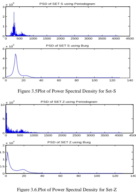
Figure 5.3.Plot of Error Histogram

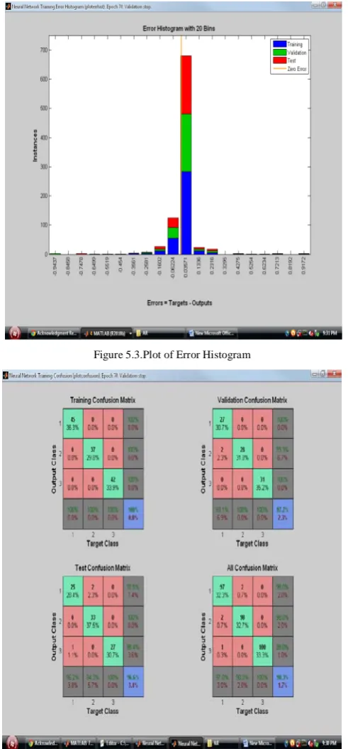
Figure 5.5. Confusion Matrix for Neural Network

The overall Confusion Matrix for the given neural network is shown below-

Table: 1

Type of Dataset Accuracy

Set-F(Epileptic Patient without Seizures) 98%

Set-S(Epileptic Patient with Seizures) 98%

SetZ (Healthy Patient without Seizures) 99%

Overall Accuracy of the Network 98.3%

VI. CONCLUSIONS

In our research we have designed a soft computing based expert system for classification of epileptic and non epileptic

EEG signals of 300 samples of data. The overall conclusion can be summarized in following points-:

a. An Automated Epileptic Classification system is

developed using Statistical features extraction and Soft Computing based classification tool.

b. Total 300 samples of individual patients were analyzed as 100 samples from each Epileptic, Pre-epileptic and Normal patients.

c. Total 25 features for wavelet features were selected to develop features input vector for classifier.

d. Classification process is carried out using SCGA- Back Propagation Neural Network Classifier.

e. Overall efficiency of 98.3 percent is achieved in the classification process .

VII. REFERENCES

[1]. Automated Epileptic Seizure DetectionMethods: A Review StudyAlexandros T. Tzallas, Markos,,Intech-Open 2011

[2]. Tzallas, A. T., Tsipouras, M. G., & Fotiadis, D. I. (2009). Epileptic seizure detection in EEGs using time-frequency analysis. IEEE Trans Inf Technol Biomed, 13(5), 703-710.

[3]. Tzallas, A. T., Tsipouras, M. G., & Fotiadis, D. I. (2007b). The use of time-frequencydistributions for epileptic seizure detection in EEG recordings. Conf Proc IEEE EngMed Biol Soc, 2007, 3-6.

[4]. Utility of multilayer perceptron neural network classifiers inthe diagnosis of the obstructive sleep apnoea syndrome from nocturnal oximetry J. Víctor Marcos computer methods and programs in biomedicine 92 (2008) 79–89, Elsevir.

[5]. Spectral Analysis of sEMG Signals to Investigate Skeletal Muscle FatigueParmod Kumar, Anish Sebastian, 2011 50thIEEE Conference on Decision and Control andEuropean Control Conference (CDC-ECC)Orlando, FL, USA, December 12-15, 2011

[6]. Real-time brain oscillation detection and phase-locked stimulation using autoregressive spectral estimation and time-series forward prediction. IEEE Trans Biomed Eng. Author manuscript; available in PMC 2012 July 31.

[7]. Spectral analysis of Signals Petre Stoica and Randolph Moses PRENTICE HALL, 2004

[8]. ModelSelection and the Principle Of MinimuDescription

Length MarkH.Hansenand BinYu,2001

[9]. Institute for Signal and Information Processing

www.isip.piconepress.com/courses/msstate.

[10]. Automated detection of pd resting tremor using psd with recurrent neural network classifier. http://www.ukessays.co.uk/essays/engineering/diagnosis-of -parkinsons-disease .php. 2011

[11]. I. Daubechies, “The wavelet transform, time-frequency loc alization and signal analysis,”IEEE Trans. on Information Theory, vol. 36, no.5, pp. 961-1005, 1990.

[12]. Adaptive neuro-fuzzy inference system for classification of EEG signals using wavelet coefficientsInan Guler ,Elif Derya Ubeyli Journal of Neuroscience Methods Elsevir (2005)

Short Bio Data for the Authors

Mr. Ashish Raj is M.Tech student at ITM University Gwalior, India. His field of interest & research includes Signal Processing and Soft Computing.

Mr.Manoj Kumar Bandil is working as Associate .Prof. In Department of Electrical Engineering at Institute Of Information Technology and Management (ITM-GOI),

Gwalior, India. His field of interest & research includes Biomedical Instrumentation System, EEG and inclusion of soft computing techniques in biomedical signal processing.