3821
Taguchi Analysis of EDM Parameters on Surface
Roughness of Al-SiC 6061 Metal Matrix Composite
Rohit Sharma
1, Vivek Aggarwal
2, H. S. Payal
3Mechanical Engineering1,2,3, IKGPTU, Kapurthala1, IKGPTU, Kapurthala2, Himalayan School of Engineering
and Technology, SRHU, Dehradun3
Email: [email protected], [email protected], [email protected]
Abstract-Wire EDM process is a good method to machine extremely hard alloys, for example, the Al SiC metal matrix composites which are rated as one of the most commonly used metal matrix composites today. This research work studies important parameters in the wire electric discharge machining of Al SiC 6061 metal matrix composite. The MMC specimens studied in this research work were fabricated with the stir casting process. Taguchi approach was employed to study the machining parameters during the machining process and to minimize the surface roughness values of the surfaces obtained by wire EDM machining. It was found out that out of the seven factors used in this study, gap voltage is the most prominent factor which influences the obtained surface roughness values. Comparatively, a very low value of surface roughness (Rq) was obtained during
confirmation test.
Keywords-Wire EDM; Composites; Al SiC; 6061; MMC; Surface Roughness; Taguchi; Orthogonal Arrays
1. INTRODUCTION
There are a total of seven main factors that influence the surface roughness value of a surface during the machining done by wire EDM process. These factors have been studied in this research work, six out of which are namely the nozzle workpiece distance, the wire feed rate at which the machining wire approaches the workpiece in order to machine it, the machining current which is made to pass through the wire and workpiece gap, the gap voltage generated between the wire and the workpiece, the wire tension of the machining wire, and the dielectric flow rate at which the dielectric is incident upon the machined area of the workpiece from the upper nozzle. Amongst these six factors, the first two factors have been studied at two levels, and the remaining four factors have been studied at four levels each. The Al SiC 6061 MMC that has been used in this work is a metal matrix composite (MMC) in which SiC particles have been used as a reinforcement phase. The percentage of SiC particles has also been studied at two levels of 5% and 10% SiC as the work piece composition, totalling the number of factors studied as seven.
Design of experiments in this work have been done in accordance with the Taguchi technique which makes use of Orthogonal Arrays. The most favourable levels of each of the abovementioned seven factors have been found out. Confirmatory test results have conducted, and the analysis of results has also been done.
1.1.The Wire EDM
Since a long time ago, researchers have attempted to employ non-conventional machining processes such as EDM, WEDM, and AWJM which are used for machining hard and high strength alloys [1]. The origin of electrical discharge machining goes back to 1770 when English scientist Joseph Priestly discovered the erosive effect of electrical discharges on metals [2]. In a Wire Electrical Discharge Machining (WEDM), the tool electrode is a continuously moving conductive wire over an electrically conducting workpiece. The practical technology of the WEDM process is based on the conventional EDM sparking phenomenon utilising the widely accepted non-contact technique of material removal [3]. Functions like wire feed, table movement, dielectric circulation and power can all be controlled through a keyboard. The mechanism of metal removal in Wire Electrical Discharge Machining involves the complex erosion effect from electric sparks generated by a pulsating direct current supply generated between the conductive wire and the work piece. Water is usually used as a dielectric in WEDM. Water is advantageous as a dielectric in this process because of its less viscosity and rapid cooling rate.
The wire EDM machine used for this work was Electra Supercut. This machine uses a brass wire of diameter 0.2 mm as cutting wire and deionized water as dielectric which is continuously circulated through the machine and filtration unit in a closed circuit.
3822
Metal matrix composites (MMCs) generally consist oflightweight metal alloys of aluminium, magnesium, or titanium, reinforced with ceramic particulate, whiskers, or fibres. The reinforcement is very important in an MMC because it determines its mechanical properties, cost, and performance. Compared with the unreinforced metal, MMCs have significantly greater stiffness and strength. However, these properties are obtained at the cost of lower ductility and toughness [4].
The aluminium industry has evolved over the past 100 years (i.e. year 1900 onwards) from the limited production of alloys and products to the high-volume manufacturing of a wide variety of products. Later, the introduction of alloy alumimium 6061 (also known as 61S) in 1935 filled the need for medium-strength, heat-treatable products with good corrosion resistance which could be welded or anodized. Alloy 6061 evolved after its initial development, the corrosion resistance of alloy 6061 even after being welded made it popular in early railroad and marine applications, and it is still used for a variety of products. The ease of hot working and low quench sensitivity are advantages in forged automotive and truck wheels. Unlike the harder aluminium-copper alloys, 6061 components can be easily fabricated by extrusion, rolling, or forging. Also made from alloy 6061 are structural sheets and tooling plates produced for the flat-rolled products market, extruded structural shapes, rods, bars, tubings, automotive drive shafts, and aircraft structures.
The Al SiC 6061 Metal Matrix Composite (MMC) used in this research work has the alloy of alumimium 6061 as its matrix phase and particles of SiC with 220 mesh size as its reinforcement phase. The two variations studied in this work are those of 5% SiC and of 10% SiC compositions, respectively. The specimens used in this work had been prepared by the stir casting process.
2. PREPARATION OF THE SPECIMENS
[image:2.595.312.521.468.689.2]In order to confirm the composition of the aluminium 6061 alloy, its spectrometry test was carried out as per the ASTM E1251-2011 test method. Two square prisms had been cut from the alloy piece for this purpose on a wire EDM machine, as have been depicted in Figure 1.
Fig. 1. Two square prisms were taken from the alumimium 6061 alloy piece in order to carry out spectrometry analysis.
The results were tallied with the available data of Al 6061 alloy's chemical composition, after which, this alloy piece was used for preparation of Al SiC 6061 specimens by the stir casting process. The results of this test have been shown in Table 1.
Table 1. Spectrometry test results of alumimium 6061 alloy.
Element Cu Mg Si Fe Ni Mn
Value (%)
0.203 0
0.933 0
0.784 0
0.304 0
0.003 2
0.083 6
Element Zn Pb Sn Ti Cr Al
Value (%)
0.056 1
0.027 0
< 0.010 0
0.068 9
0.047 2
Rem.
In the specimen preparation stage, the alumimium 6061 alloy piece which was taken as the matrix phase was cut into smaller blocks so as to facilitate melting in a vertical muffle furnace. SiC powder of 220 mesh size had been taken as the reinforcement phase. Both of them had been accurately weighed for the 5% and 10% composition specimens, respectively. Also, a magnesium ribbon strip was added which had been 1% by weight of alloy. The alumimium 6061 blocks, the SiC powder, and the magnesium wire used for the preparation of specimens have been shown in Figure 2.
[image:2.595.82.284.658.820.2]3823
During casting, accurately weighed alumimium 6061blocks were placed in a crucible and heated to a temperature of about 8500C. Preheating of
[image:3.595.315.515.271.428.2] [image:3.595.81.285.359.501.2]reinforcement results in uniform distribution and better mechanical properties [5]. SiC particles are preheated in this process so as to expel moisture and other volatile contaminants from them. An accurately weighed quantity of magnesium ribbon to the hot crucible was then done which was slightly problematic as it caught fire on incident to furnace heat but was immediately sunk in the molten slurry with an m.s. rod (the operators had previous experience of doing so). An electrical motor operated stirrer of graphite was then left to rotate in it for some time, as shown in Figure 3.
[image:3.595.316.489.539.738.2]Fig. 3. A stirrer of graphite was used to rotate the liquefied contents of the crucible placed in the furnace. The molten metal was then poured into two specially prepared cylinder moulds, as shown in Figure 4.
Fig. 4. Some slag that had been floating on the molten metal was removed with an m.s. rod, and the remaining molten metal was poured in specially made cylinder moulds.
After allowing to cool down and solidify for some time, the first solidified casting was removed from its cylinder mould. The process was repeated for the other casting, giving two castings, the one with 5% SiC content composition and the other one with 10%
SiC content composition, respectively. The surfaces of these castings were pitted and had been having inaccurate dimensions at that time. Hence, they were turned on a lathe. These specimens have been shown in Figure 5.
Fig. 5. The two castings after being turned to accurate dimensions of 14 mm diameter.
[image:3.595.101.254.627.770.2]This SEM analysis of one of these specimens was done on a Scanning Electron Microscope of JEOL make whose results have been shown in Figure 6.
Fig. 6. SEM photograph of the specimen.
3. DESIGN OF EXPERIMENTS
Experiment is defined as a test to establish a hypothesis. To design an experiment is to develop a scheme or layout of the different conditions to be studied. Design of Experiments is another name given to Factorial Experiments that involve more than one
3824
An experimental design should satisfy two objectives.Firstly, the number of trials should be minimum, and
secondly, conditions of each trial must be specified. Taguchi design of experiments is such an efficient test strategy that possesses some advantages because of a balanced arrangement [6].
3.1. The Taguchi technique and the Orthogonal arrays
The Taguchi technique makes use of Orthogonal Arrays (OAs). An OA is a mathematical invention recorded by Jacques Hadamard, a French mathematician in as early as 1897 [6]. The use of Latin squares Orthogonal Arrays (a type of Orthogonal Array).
The Taguchi technique of layout of the conditions (Design of Experiments) involving multiple factors was first proposed by the Englishman Sir RA Fischer in the 1920s. This method is popularly known as the Factorial Design of Experiments. It may either be a
Full Factorial Design or else a Fractional Factorial Design. A Full Factorial Design identifies all possible combinations for a given set of factors. In a Full Factorial Design, seven factors, each at two levels shall need 27 = 128 experiments. In order to reduce
such a large number of experiments to a practical level, only a small set from all the possibilities is selected in the Fractional Factorial Design. This is done with the use of Orthogonal Arrays. An Orthogonal Matrix Array, also called the Orthogonal Array, abbreviated as OA is defined as such a Fractional Factorial Matrix that it assumes a balanced, fair comparison of levels of any factor in which all columns can be evaluated independently of one another [6].
The term levels of various factors is defined as the setting of various factors in a factorial experiment [6]. It is generally considered wise to think the level 1 is lesser in numerical value than level 2; both levels of a factor should have the same units. It can be seen that Taguchi method has been successfully used in the optimization of machining parameters [7]. In fact, optimization of process parameters is the key step in the Taguchi method in achieving high quality without increasing the cost [8].
4. CONDUCTING THE EXPERIMENTS
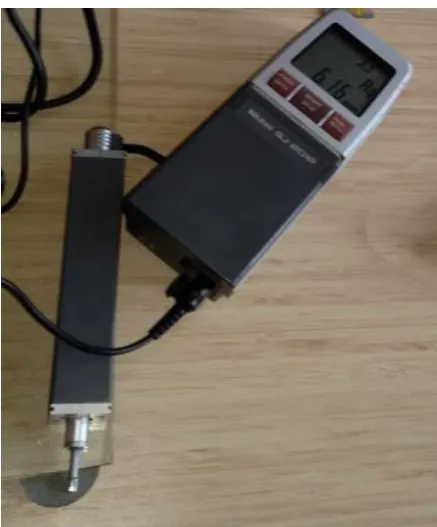
After the design of experiments, when each experimental run was decided in terms of various parameters and their levels, the specimens were mounted on the wire EDM machine, and machining cuts were performed (48 in number) in accordance to the conditions described by the l-16 orthogonal array (pronounced as ell sixteen). Each of these cuts was 14 mm deep and all these cuts were placed mutually at an axial distance of 2.5 mm. The machining of such cuts on cylindrical specimens gave semi circular shaped pieces, one of which is shown in Figure 7. During experimentation, after machining each cut, the machining parameter levels were changed every time as per the Taguchi design of experiments and the next cut was then machined in the specimen. Machining cuts were performed on both the specimens, as per the design of experiments. After machining all the cuts on both the specimens, surface roughness testing was carried out on the machined surfaces brought out by the machining cuts. In order to get more accurate results, surface roughness measurement was done at five places on each machined surface, and their average was then taken. A Mitutoyo make surftest meter SJ-201-P was used for this purpose, and roughness of machined surfaces was measured in units of µm on the scale of Rq. This has been shown in
[image:4.595.71.290.129.393.2]Figure 7 below.
Fig. 7. Photograph of the roughness testing of one of the semi circular shaped pieces being carried out.
3825
Table 2. Average surface roughness obtained duringmachining at each setting of Orthogonal Array (numbered 1 to 16).
N u m be r of cu t Surface roughne ss values of specime n pieces (number ed 1 to 16)
(μm)
Surface roughne ss values of specime n pieces (number ed 17 to 32)
(μm)
Surface roughne ss values of specime n pieces (number ed 33 to 48) (μm) Average surface roughnes s (OA settings of 1 to 16) (μm)
1 6.78 4.87 4.85 5.5
2 4.2 5.88 4.93 5
3 6.75 7.47 6.26 6.83
4 6.48 8.33 8.58 7.8
5 4.86 4.61 4.45 4.64
6 3.97 6.17 4.09 4.74
7 4.53 5.32 4.66 4.84
8 8.09 6.66 6.21 6.99
9 4.96 5.4 3.76 4.71
10 7.5 4.59 4.15 5.41
11 4.54 6.82 5.02 5.46
12 7.23 6.6 7.27 7.03
13 4.51 4.05 4.53 4.36
14 5.8 4.48 4.25 4.84
15 5.15 4.83 3.91 4.63
16 7.71 6.12 4.89 6.24
[image:5.595.70.302.685.767.2]As per the standard method of Taguchi analysis of orthogonal arrays, these 16 values had been placed on the right side of the l-16 orthogonal array, as shown in Table 3 below.
Table 3. Orthogonal Array l-16 for surface roughness.
Lev el 4 1. 25 A 72 V 12 00 g 2. 5 l.p .m .
Lev 1. 68 11 2.
el 3 00
A
V 00 g 0 l.p .m . Lev el 2 10 % Si C 50 m m 5 m/ mi n 0. 75 A 64 V 10 00 g 1. 5 l.p .m . Lev el 1 5 % Si C 40 m m 3 m/ mi n 0. 50 A 60 V 90 0 g 1. 0 l.p .m . Exp . trial no. W or k pi ec e co m po sit io n N oz zle w or kp ie ce di st an ce W ire fe ed ra te M ac hi ni ng C ur re nt G ap vo lta ge W ire te ns io n Di el ec tri c flo w ra te F ac to r A F ac to r B F ac to r C F ac to r D F ac to r E F ac to r F F ac to r G Averag e surface roughn ess (μm)
1 1 1 1 1 1 1 1 5.5
2 1 2 2 1 2 2 2 5
3 2 1 2 1 3 3 3 6.83
4 2 2 1 1 4 4 4 7.8
5 2 2 1 2 1 2 1 4.64
6 2 1 2 2 2 1 2 4.74
7 1 2 2 2 3 4 4 4.84
8 1 1 1 2 4 3 3 6.99
9 1 2 2 3 1 3 4 4.71
10 1 1 1 3 2 4 3 5.41
11 2 2 1 3 3 1 2 5.46
12 2 1 2 3 4 2 1 7.03
13 2 1 2 4 1 4 2 4.36
14 2 2 1 4 2 3 1 4.84
15 1 1 1 4 3 2 4 4.63
16 1 2 2 4 4 1 3 6.24
3826
5. ANALYSIS OF RESULTS
5.1. Calculations for the Average Effects of surface roughness
The calculations of the Average Effects of various parameters affecting surface roughness have been shown below at various levels.
The Average Effects of Work piece composition, A1=
(5.5+5+4.84+6.99+4.71+5.41+4.63+6.24)/8 =5.415,
A2=
(6.83+7.8+4.64+4.74+5.46+7.03+4.36+4.84)/ 8
=5.713.
The Average Effects of Nozzle workpiece distance, B1=
(5.5+6.83+4.74+6.99+5.41+7.03+4.36+4.63)/ 8
= 5.686, B2=
(5+7.8+4.64+4.84+4.71+5.46+4.84+6.24)/8 = 5.441.
The Average Effects of Wire feed rate, C1=
(5.5+7.8+4.64+6.99+5.41+5.46+4.84+4.63)/8 = 5.659,
C2=
(5+6.83+4.74+4.84+4.71+7.03+4.36+6.24)/8 = 5.469.
The Average Effects of Machining Current, D1 = (5.5+5+6.83+7.8)/4
= 6.282,
D2= (4.64+4.74+4.84+6.99)/4
= 5.303,
D3=(4.71+5.41+5.46+7.03)/4
= 5.653,
D4=(4.36+4.84+4.63+6.24)/4
= 5.018.
The Average Effects of Gap voltage, E1=(5.5+4.64+4.71+4.36)/4
= 4.803,
E2 =(5+4.74+5.41+4.84)/4
= 4.998,
E3=(6.83+6.84+5.46+4.63)/4
= 5.440,
E4=(7.8+6.99+7.03+6.24)/4
= 7.015.
The Average Effects of Wire tension, F1=(5.5+4.74+5.46+6.24)/4
= 5.485,
F2 = (5+4.64+7.03+4.63)/4
= 5.325,
F3 = (6.83+6.99+4.71+4.84)/4
= 5.843,
F4=(7.8+4.84+5.41+4.36)/4
= 5.603.
The Average Effects of Dielectric flow rate, G1=(5.5+4.64+7.03+4.84)/4
= 5.503,
G2=(5 +4.74+5.46+4.36)/4 =
4.890,
G3=(6.83+6.99+5.41+6.24)/4
= 6.368,
G4= (7.8+4.84+4.71+4.63)/4
=5.495.
[image:6.595.73.290.200.765.2]These Average Effects have been shown in Table 4.
Table 4. The Average Effects of various factors affecting surface roughness in Wire EDM process.
Factor Factor descri ption
Lev el 1,
L1 Lev el 2,
L2 Lev el 3,
L3
Level 4, L4
A Work
piece compo sition
5.4 15
5.7 13
- -
B Nozzle
workpi ece distanc e
5.6 86
5.4 41
- -
C Wire
feed rate
5.6 59
5.4 69
- -
D Machin
ing Current
6.2 82
5.3 03
5.6 53
5.018
E Gap
voltage 4.8 03
4.9 98
5.4 40
7.015
F Wire
tension 5.4 85
5.3 25
5.8 43
5.603
G Dielect
ric flow rate
5.5 03
4.8 90
6.3 68
5.495
5.2. Calculations for sum of squares of factors and their percentage contribution
Based on the Table 4 given above, next, the sum of square of each factor was calculated. The relation used here is shown in Eq. (1),
SS =
∑
x−xm 2
[image:6.595.306.534.257.598.2]n−1 (1), where all terms have their usual notations.
Table 5.1. Calculating Means of levels
Fact or
Factor descripti on
Lev el 1,
L1 Lev el 2,
L2 Lev el 3,
L3 Lev el 4,
L4 Mean of Level s (xm)
A Work
piece
5.4 2
5.7 1
[image:6.595.306.533.260.594.2]3827
composition
B Nozzle
workpiec e distance 5.6 9 5.4 4
- - 5.56
C Wire feed rate
5.6 6
5.4 7
- - 5.56
D Machinin
g Current 6.2 8
5.3 5.6 5
5.0 2
5.56
E Gap
voltage
4.8 5 5.4
4 7.0 2
5.56
F Wire
tension 5.4 9 5.3 3 5.8 4
5.6 5.56
G Dielectric flow rate
5.5 4.8 9
6.3 7
5.5 5.56
[image:7.595.70.297.319.704.2]The Means of Levels of various factors are then used to find out the Percentage Contribution of each factor, as shown in Table 5.2 and Table 5.3.
Table 5.2. Calculating Σ for Percentage Contribution
Factor Factor descri ption
(L1 -xm) 2
(L2 -xm) 2
(L3 -xm) 2
(L4 -xm) 2
Σ
A Work
piece compo sition 0.0 222 01 0.0 222 01
- - 0.044
402
B Nozzle
workpi ece distanc e 0.0 150 06 0.0 150 06
- - 0.030
013
C Wire
feed rate 0.0 090 25 0.0 090 25
- - 0.018
050
D Machin
ing Current 0.5 155 24 0.0 681 21 0.0 079 21 0.2 981 16 0.889 682
E Gap
voltage 0.5 791 21 0.3 203 56 0.0 153 76 2.1 054 01 3.020 254
F Wire
tension 0.0 062 41 0.0 571 21 0.0 778 41 0.0 015 21 0.142 724
G Dielect
ric flow rate 0.0 037 21 0.4 542 76 0.6 464 16 0.0 047 61 1.109 174
Table 5.3. Calculations for Percentage contribution
Factor Σ D. F. Sum of squares Contri bution Contrib ution (%)
A 0.044
402
1 0.04440 2
0.0245 2.45
B 0.030
013
1 0.03001 3
0.0166 1.66
C 0.018
050
1 0.01805 0
0.0100 1
D 0.889
682
3 0.29656 1
0.1636 16.36
E 3.020
254
3 1.00675 1
0.5553 55.53
F 0.142
724
3 0.04757 5
0.0262 2.62
G 1.109
174
3 0.36972 5
0.2039 20.39
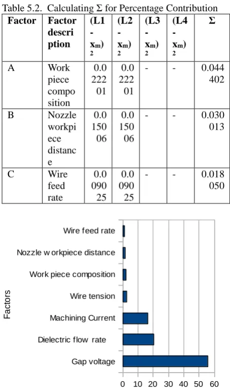
The percentage contribution of all these factors have been shown in Figure 8. It is clearly seen that Gap Voltage has maximum effect on the surface roughness values, followed by Dielectric flow rate and machining current, respectively.
Fig. 8. Percentage contribution of various factors in wire EDM machining of Al SiC 6061 MMC.
5.2.Calculations for Main Effects of surface roughness
In order to calculate the Main Effects of various parameters affecting surface roughness, the Average Effects of each factor are plotted on a graph, one by one. This is done by placing the Average Effects along the x-axis and the factor levels along the y-axis of all the factors. The plots obtained have been shown below.
5.3.1.Main Effects of the factor of workpiece composition
Gap voltage Dielectric flow rate Machining Current Wire tension Work piece composition Nozzle w orkpiece distance Wire feed rate
0 10 20 30 40 50 60
Percentage Contribution
F
a
ct
o
3828
Fig. 9. A graphical plot showing the Main Effects offactor A (the percentage of SiC in Al SiC MMC specimens). X axis has 5% SiC composition as A1 and 10% SiC composition as A2 whereas Y axis shows Average Effects in units of Rq.
The surface roughness value needs to be minimized. Hence, from Figure 9, we see that the factor level that shall result in minimum value of surface roughness corresponds to A1.
5.3.2.Main Effects of the factor of Nozzle workpiece
[image:8.595.312.507.276.398.2]distance
Fig. 10. A graphical plot showing the Main Effects of factor B (Nozzle workpiece distance). Y axis has Average Effects in units of Rq. X axis has 40 mm as
level B1 and 50 mm as level B2 in units of mm.
The value of surface roughness needs to be minimized. Hence, from Figure 10, we see that the factor level that shall result in minimum value of surface roughness corresponds to B2.
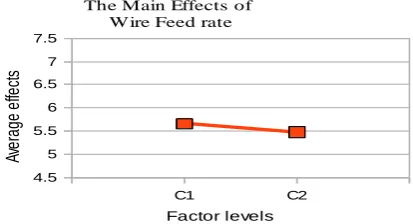
[image:8.595.82.289.395.507.2]5.3.3. Main Effects of the factor of wire feed rate
Fig. 11. A graphical plot showing the Main Effects of factor C (Wire feed rate). Y axis has Average Effects in units of Rq. X axis has 3 m/min as level C1 and 5
m/min as level C2.
The value of surface roughness needs to be minimized. Hence, from Figure 11, we see that the factor level which shall result in minimum value of surface roughness corresponds to C2.
5.3.4. Main Effects of the factor of Machining current
Fig. 12. A graphical plot showing the Main Effects of
factor D (machining current). Y axis has Average Effects in units of Rq. X axis has machining current as
a factor at levels D1, D2, D3, and D4 in units of ampere.
The value of surface roughness needs to be minimized. Hence, from Figure 12, we see that the factor level which shall result in minimum value of surface roughness corresponds to D4.
5.3.5. Main Effects of the factor of gap voltage
Fig. 13. A graphical plot showing the Main Effects of factor E (gap voltage). Y axis has Average Effects in
A1 A2
4.5 5 5.5 6 6.5 7 7.5
The Main Effects of Workpiece compos ition
Factor levels
Av
era
ge
e
ffe
ct
s
D1 D2 D3 D4
4.5 5 5.5 6 6.5 7 7.5
The Main Effects ) of Machining Current
Factor levels
Av
era
ge
e
ffe
ct
s
E1 E2 E3 E4
4.5 5 5.5 6 6.5 7 7.5
The Main Effects of Gap Voltage
Factor levels
A
ve
ra
g
e
e
ff
e
ct
s
B1 B2
4.5 5 5.5 6 6.5 7 7.5
The Main Effects of Nozzle workpiece dis tance
Factor levels
Av
era
ge
e
ffe
ct
s
C1 C2
4.5 5 5.5 6 6.5 7 7.5
The Main Effects of Wire Feed rate
Factor levels
Av
era
ge
e
ffe
ct
[image:8.595.318.517.435.591.2]3829
units of Rq. X axis has gap voltage as a factor at levelsE1, E2, E3, and E4 in units of volts.
The value of surface roughness needs to be minimized. Hence, from Figure 13, we see that the factor level which shall result in minimum value of surface roughness corresponds to E1.
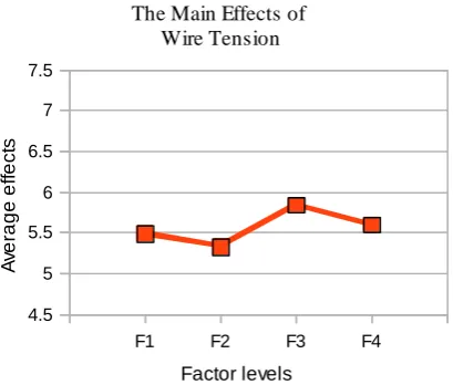
5.3.6. Main Effects of the factor of wire tension
Fig. 14. A graphical plot showing the Main Effects of factor F (wire tension ). Y axis has Average Effects in units of Rq and X axis has (wire) tension as a factor at
levels F1, F2, F3, and F4 in units of grams.
The value of surface roughness needs to be minimized. Hence, from Figure 14, we see that the factor level which shall result in minimum value of surface roughness corresponds to F2.
[image:9.595.82.287.208.382.2]5.3.7. Main Effects of the factor of dielectric flow rate
Fig. 15. A graphical plot showing the Main Effects of factor G (dielectric flow rate ). Y axis has Average Effects in units of Rq. X axis has dielectric flow rate as
a factor at levels G1, G2, G3, and G4 in units of l.p.m.
The value of surface roughness needs to be minimized. Hence, from Figure 15, we see that the factor level which shall result in minimum value of surface roughness corresponds to G2.
From the graphical plots shown above, we see that the levels of various factors which shall result in a low value of surface roughness corresponds to A1B2C2
D4E1 F2 G2..
[image:9.595.84.284.548.711.2]The levels of various factors that shall result in minimum value of surface roughness can be shown in tabular form, as in Table 6.
Table 6. Levels of factors for minimum value of surface roughness.
Factor Factor Description
Levels for minimum surface roughness
A Work piece
composition
SiC 5%
B Nozzle workpiece distance
50 mm
C Wire feed rate 5 m/min
D Machining
Current
1.25 A
E Gap voltage 60 V
F Wire tension 1000 g
G Dielectric flow
rate
1.5 l.p.m.
It is deemed that the above mentioned levels of the given factors which shall result in minimum value of surface roughness.
5.3.Calculations for Projection of optimal performance
According to the usual notations, here, Total number of observations, N = 16 Sum total of all observations, T
= 5.5 + 5 + 6.83 + 7.8 + 4.64 + 4.74 + 4.84 + 6.99 + 4.71 + 5.41 + 5.46 + 7.03 + 4.36 + 4.84 + 4.63 + 6.24
= 89.02.
Using the relation for optimal performance,
Yoptimal = T/N + (A1 - T/N) + (B2 - T/N) +
(C2 - T/N) + (D4 - T/N) + (E1 - T/N) + (F2 - T/N)
+ (G2- T/N)
= 5.56 + (5.42-5.56) + (5.44-5.56) + (5.47- 5.56) + (5.02-5.56) + (4.8-5.56) + (5.33-5.56) + (4.89-(5.33-5.56)
= 5.56+ (- 0.14) + (-0.12) + (- 0.09)+ (-0.54) + (-0.76) + (-0.23) + (-0.67)
= 3.01 μm.
F1 F2 F3 F4
4.5 5 5.5 6 6.5 7 7.5
The Main Effects of Wire Tension
Factor levels
A
ve
ra
g
e
e
ff
e
ct
s
G1 G2 G3 G4
4.5 5 5.5 6 6.5 7 7.5
The Main Effects of Dielectric flow rate
Factor levels
A
ve
ra
g
e
e
ff
e
ct
3830
6. CONFIRMATION TESTS
[image:10.595.72.297.179.499.2]In order to confirm the accuracy of predicted values, a total of three tests were performed and hence, three specimen pieces were obtained by wire EDM machining at the experimental factors which have been described in Table 6. Surface roughness values were measured on all these three specimen pieces at five random points on their surfaces and their average was taken. Then the average surface roughness values of these three specimen pieces were taken. These calculations have been shown in Table 7.
Table 7. Confirmation test results for surface roughness
S p e ci m e n p ie c e n o .
Measured values
(µm)
Mean values
(µm)
Average value
(µm) 1st 2nd 3rd 4th 5th
1 4.1 6
3.5 1
3.1 8
3.7 3
3.4 2
3.6 3.52
2 3.2 1
2.8 3.3 5
3.8 3
3.8 8
3.41
3 3.4 3.1 2
3.6 1
3.5 1
3.5 4
3.54
The value of average surface roughness obtained during confirmation tests was compared with the values earlier obtained using the relation for optimal performance. Actual values were 116.94% of the calculated values which are quite satisfactory. Their comparison has been shown graphically in Figure 16.
Fig. 16. Comparison of predicted values which had
been obtained theoretically by mathematical relations with those obtained during the confirmation tests.
7. CONCLUSIONS
High energy material removal methods allow the machining process to take a major leap to increase the removal rate. However, these methods also have a significant impact on the part integrity as they alter the state of the surface after processing by the introduction of defects or surface residuals, generate unfavourable tensile residual stresses or influence the surface roughness [9]. In this work, it became evident that various factors affect the surface roughness of machined surfaces of Al SiC 6061 MMC done by wire EDM machine. This work shows that how seven of these factors, namely, workpiece composition, nozzle workpiece distance, wire feed rate, machining current, gap voltage, wire tension, and dielectric flow rate, can be used to control the roughness values of surfaces being machined. As one of these factors is work piece composition, we also found out the composition of workpiece which shall result in a better value of surface roughness.
The percentage contribution of these factors also had been worked out, which gave the gap voltage as the most dominant factor affecting the surface roughness values.
The predicted values which were obtained by relations in a theoretical way were very close to the values obtained during the confirmation tests which authenticates this research work.
This study shows the way to obtain better surfaces, having lesser values of surface roughness which are desirable for use in numerous mechanical processes.
8. ACKNOWLEDGMENTS
In addition to research guide Dr. Vivek Aggarwal (IKGPTU, Julundhur) and (Prof.) Dr. H.S. Payal (Dehradun), the author would like to extend sincere gratitude to Dr. Naveen Beri (BCET, Gurdaspur), Dr. Sarabjeet Singh Sidhu (BCET), Professor Alakesh Manna (PEC, Chandigarh), Mr. Ram Niranjan (Lab Incharge, PEC), Mr. Vivek (PEC), Dr. Kanwaljeet Singh Khas (Researcher, IIT, Delhi), Aman and Dhanraj (Wire EDM operators), and Er. Aman, Mr. Chhagan and Mr. R.K. Jindal, Wire EDM owners, Chandigarh, along with Mr. Nirmal Singh, (who helped me with the hardness testing machine), Kharar who are people who proved helpful at some or the other stage of this research work.
REFERENCES
[1] Shashikant, A. Roy, and K. Kumar. “Effect and Optimization of Various Machine Process Parameters on the Surface Roughnes in EDM for an EN19 material using Response Surface
Predicted value (Calculated) Actual value 0
[image:10.595.82.284.615.768.2]E-ISSN: 2321-9637
Available online at
www.ijrat.org
3831
Methodology”. Procedia Mater. Sci., volume 5,pages 1702-1709, 2014.
[2] D. Scot, S. Boyina, and K. Rajurkar. “Analysis and optimization of parameter combinations in Wire Electric Discharge Machining”. Department of Industrial and Management Systems Engineering, University of Nebraska-Lincoln, USA, volume 19/11, pages 2189–2207, 1990. [3] R. Garg and H. Singh. “Optimisation of process
parameters for gap current in wire electrical discharge machining". Int. J. of Manufacturing Technology and Management, volume 25, pages 161-175, 2012.
[4] “Advanced Materials by design”. Washington DC, US Government Printing Office, chapter 1, page 9.
[5] S. Shanker. “A review on properties of conventional and metal matrix composite materials in manufacturing of disc brake”. Materials Today Proceedings, volume 5, issue 2, part 1, pages 5864-5869, 2018.
[6] P. Ross. “Taguchi Techniques for Quality Engineering”. Mc Graw Hill Professional, New York, 1996.
[7] Y. Ahmed, H. Youssef, H. Hofy, and M. Ahmed. “Prediction and Optimization of Drilling Parameters in Drilling of AISI 304 and AISI 2205 Steels with PVD Monolayer and Multilayer Coated Drills”. J. Manuf. Mater. Process, volume 2(1), page 16, 2018.
[8] C. Schneider, C. Lisboa, R. Silva, and Lermen. “R.T. Optimizing the Parameters of TIG-MIG/MAG Hybrid Welding on the Geometry of Bead Welding Using the Taguchi Method”. J. Manuf. Mater. Process, volume 1, page 14, 2017. [9] J. Holmberg, A. Wretland, and L. Berglund.