Fuzzy Image Segmentation Using Membership Connectedness

Volume 2008, Article ID 417293,13pages doi:10.1155/2008/417293

Research Article

Fuzzy Image Segmentation Using Membership Connectedness

Maryam Hasanzadeh and Shohreh Kasaei

Computer Engineering Department, Sharif University of Technology, Tehran 11155-9517, Iran

Correspondence should be addressed to Shohreh Kasaei,[email protected]

Received 27 July 2008; Revised 11 September 2008; Accepted 15 October 2008

Recommended by Stephen Marshall

Fuzzy connectedness and fuzzy clustering are two well-known techniques for fuzzy image segmentation. The former considers the relation of pixels in the spatial space but does not inherently utilize their feature information. On the other hand, the latter does not consider the spatial relations among pixels. In this paper, a new segmentation algorithm is proposed in which these methods are combined via a notion called membership connectedness. In this algorithm, two kinds of local spatial attractions are considered in the functional form of membership connectedness and the required seeds can be selected automatically. The performance of the proposed method is evaluated using a developed synthetic image dataset and both simulated and real brainmagnetic resonance image(MRI) datasets. The evaluation demonstrates the strength of the proposed algorithm in segmentation of noisy images which plays an important role especially in medical image applications.

Copyright © 2008 M. Hasanzadeh and S. Kasaei. This is an open access article distributed under the Creative Commons Attribution License, which permits unrestricted use, distribution, and reproduction in any medium, provided the original work is properly cited.

1. INTRODUCTION

Image segmentation is one of the most challenging and critical problems in image analysis. Segmentation processes aim at partitioning the image plane into “meaningful” regions (where meaningful typically refers to separation of image regions into different semantic objects). As image segmentation is the core of many image analysis problems, any improvement in segmentation methods can lead to important impacts on many image processing and computer vision applications.

Challenges in image segmentation have encouraged researchers to develop fuzzy segmentation algorithms by considering image regions as fuzzy subsets (fuzzy objects), where an image pixel may be partially classified into multiple potential classes and the boundaries between intensities of different objects can be well defined. Here, the theory of fuzzy sets [1] is adopted to effectively model the fuzziness of image pixels which might be caused by inherent object material heterogeneity and imaging device artifacts (e.g., blurring, imposed noise, and background variation).

There are several image segmentation methods based on fuzzy concept reported in [2–4] among which fuzzy connectedness [5] and fuzzy clustering [4] are two well-known techniques for this purpose. Moreover, fuzzy

rule-based methods [2,6–8], fuzzy thresholding [3,9–11], fuzzy markov random field [12–14], and fuzzy region growing [15, 16] are also reported for region-based fuzzy segmentation.

Fuzzy connectedness is a fuzzy topological property [17] and defines how the image pixels are spatially related in spite of their gradation of intensities [18]. The classical definition of fuzzy connectedness was given by Rosenfeld in [19]. A modification to this traditional concept, called intensity

connectedness, was proposed in [20]. Fuzzy connectedness

for image segmentation was developed by Udupa and Samarasekera in [5] by notion of a fuzzy object in an N -dimensional space. In defining fuzzy objects in a given image, the strength of connectedness between every two pairs of image pixels is considered. This is determined by considering all possible connecting paths between the pair. In spite of its high combinatorial complexity, theoretical advances in fuzzy connectedness have made it possible to delineate objects via a dynamic programming close to interactive speeds on modern PCs [5].

a threshold which requires an exhaustive search cost. This issue is very critical in applications such as analysis of

mag-netic resonance (MR) images, where optimal combination

of affinity component weights varies for each slice and each subject [21] in spite of data being acquired from the same MR scanner with identical protocol. As such, in [21] a method based on dynamic weights is introduced. But, these methods depend on manual selection of object seeds (which is time consuming and may cause errors especially in multicomponent objects). As such, a method for automatic seed selection using fuzzy clustering is introduced in [22], but it also applies the fuzzy connectedness directly on the given image.

On the other hand, feature clustering that uses fuzzy clustering techniques does not take into account any spatial dependency among image pixels and consequently it is sensitive to noise. As the noise removal may eliminate some inherent image information, some methods are recently proposed for integration of spatial information in fuzzy clustering for segmentation applications [23–27].

Considering the abovementioned problems, in this paper we have proposed a new algorithm to combine fuzzy connectedness and fuzzy clustering methods for image segmentation purposes. The desired goal is using both spatial and feature space features in image segmentation. These methods might be integrated tightly in a single algorithm or combined (similar to a postprocessing approach). As these methods utilize the information of dissimilar spaces (feature or spatial) we have adopted the second possibility in this paper. The proposed algorithm is based on construction of fuzzy connectedness relation in membership images, calledmembership connectedness. Two kinds of local spatial attractions are considered in the proposed functional form of membership connectedness relation.

The construction of membership connectedness requires an initial reference pixel (seed) in the object. As the manual selection of object seeds in multicomponent and complicated objects (such as brain tissues) is very time consuming and may cause error, an automatic method for seed selection is also described.

As the seed set for fuzzy object construction can be selected automatically, if the number of objects in the image is known, the proposed algorithm can be applied completely in an unsupervised manner. Moreover, its advantages include a straightforward utilization for color and multispectral image segmentation, multiobject segmentation, and multi-seed utilization abilities. Besides, it does not assume any specific characteristic for the adopted fuzzy segmentation method.

The performance of the proposed algorithm is evaluated using a developed synthetic image dataset which contains 720 images, phantom multispectral MR images from brain-webdataset [28], andIBSRdataset of real brain MRI [29].

This paper proposes an application domain-independent segmentation algorithm and evaluates its performance on brain tissue of MR images; as this application requires accu-rate and robust segmentation results in many quantitative studies in medical image analysis. Different characteristics of the proposed segmentation algorithm are advantageous for

this application. In fact, since MR scans are often confounded by magnetic field inhomogeneities and partial volume effects (one pixel may be composed of multiple tissue types), modeling of tissues by fuzzy objects and applying fuzzy segmentation are useful in MR image analysis. In addition to the use of fuzzy connectedness idea (which has been successfully applied in medical image segmentation [18,21]), the proposed algorithm is not based on affinity function and thus the dynamic computation of its optimal parameters for each slice and each subject in MR image analysis is not required. Moreover, its ability in automatic selection of seed pixels eliminates possible manual selection errors in multicomponent and complicated brain tissues (such as peripheral cerebrospinal fluid and multiple sclerosis lesions). This paper is organized as follows. Section 2 briefly reviews the concept of fuzzy connectedness in image segmen-tation.Section 3introduces the proposed membership con-nectedness notion and segmentation algorithm. Section 4 describes experimental results, and finally Section 5 con-cludes the paper.

2. FUZZY CONNECTEDNESS AND IMAGE SEGMENTATION

Fuzzy treatment of geometric and topological concepts can be performed in two distinct manners in image segmentation [18]. The first approach applies a fuzzy image segmentation to obtain a fuzzy subset wherein every pixel has a fuzzy object membership assigned to it and then defines the geometric and topological concepts on this fuzzy subset. The second approach develops these concepts directly on the given image, which implies that these concepts have to be integrated with segmentation process.

Considering the first approach, Rosenfeld introduced some early work [19,30] which was followed by Dellepiane and Fontana [20] in an intensity connectedness-based seg-mentation method. This approach is adopted in this work.

Introducing the second approach, Udupa and Sama-rasekera [5], and Udupa and Saha [18] proposed an algo-rithm for object definition and segmentation from back-ground, based on fuzzy connectedness which is a topological construct. Fuzzy connectedness characterizes the way that image pixels are related to each other (called “hanging togetherness” in [18]) to form an object.

In the latter algorithm, fuzzy connectedness definition is based on a local fuzzy relation called affinity [18]. The affinity between two image pixels depends on their adjacency as well as their intensity-based features’ similarity which captures the local spatial relation of image pixels. The following is a general functional form of membership function (μκ) of

affinity relation (κ) as proposed in [5]:

μκ(c,d)=μα(c,d)g

μϕ(c,d),μψ(c,d)

, (1)

where (c,d) denotes a pair of pixels, μα is the adjacency

function, and μψ and μϕ represent the fuzzy relation of

allowed inhomogeneity in the desired object. The object feature-based component depends on the closeness of inten-sity features of the desired pair of pixels to the feature values expected for the desired object. These components can be combined by an appropriateg(·) function.

The global fuzzy connectedness between any two image pixels considers the strength of all possible paths between them; where the strength of a particular path is the weakest affinity between the successive pixel pairs along the path. The fuzzy connectedness relation (K) is defined by the membership function [18]

μK(c,d)=max p∈Pcd

min 1<i≤lp

μκ

ci−1,ci

, (2)

wherePcdis the set of all paths (a path is a sequence of nearby elements) connectingctod,lpis the length ofp, andciand

ci−1are two successive pixels inp.

The fuzzy object is then extracted by expanding it from the initial seed points based on the mentioned global fuzzy connectedness value. For expansion, the connectedness of each image pixel to a particular object (which is equal to the connectedness of the pixel to the initial seed set of the object) is computed. The connectedness of a pixel to a set of reference pixels is the maximum of connectedness degrees to every pixel of set [18], as defined below for setSand arbitrary pixelc,as

fKs(c)=max s∈S

μK(s,c)

. (3)

Finally, thresholding or applyingrelative fuzzy connectedness

[31] will result in a crisp object.

The above-discussed algorithm was further extended with introduction of object scale, which allowed the size of neighborhood to be changed in different image parts [32], and extended in [33] for vectorial images and in [34] for multiobject segmentation purposes. Another method, called fuzzy connectedness using dynamic weights, was proposed in [21] to introduce directional sensitivity to the homogeneity-based component to dynamically adjust linear weights in the functional form of fuzzy connectedness.

3. PROPOSED METHOD

As discussed in previous sections, fuzzy connectedness influences the segmentation result by spatio-topological consideration of the way that image pixels relate together. This advantage becomes more obvious when one compares it with feature-based segmentation algorithms (i.e., fuzzy clustering), which do not take into account any spatial dependency among image pixels. But, applying fuzzy con-nectedness directly on a gray-level image requires parameter selection and estimation of object features which often require user interaction (which is time consuming and may cause error especially in multicomponent objects). In this section, we describe a new algorithm for applying fuzzy connectedness on membership scene (defined in Section 3.1, which is resulted by an arbitrary fuzzy segmentation method) via proposed membership connectedness relation.

By this relation, fuzzy connectedness and fuzzy clustering are integrated for image segmentation purposes. These methods may be tightly integrated which result in a single algorithm or may be combined similar to a postprocessing approach. As these methods utilize the information of dissimilar spaces (feature or spatial), we have adopted the second possibility in this paper.

In this section, we start by briefly reviewing some basis definitions in Section3.1, which are required for formulation of membership connectedness relation in Section3.2. In this section, two kinds of local spatial attractions are considered in the functional form of membership connectedness that results in two different relations. Then, we discuss the main proposed segmentation algorithm in detail about seed selec-tion method and fuzzy object expansion algorithm. Finally, the advantages of the proposed segmentation algorithm are introduced.

3.1. Basic definitions

In this subsection, a basic set of definitions are presented to provide the preliminaries of the membership connectedness formulation. First, we define the membership scene by following the terminology used in [18] and then briefly describe thefuzzy C-means(FCM) clustering method.

LetXbe any reference set. A fuzzy subsetAofXis a set of ordered pairsA= {(x,μA(x))|x∈X}, whereμA :x →

[0, 1] is the membership function ofAinX(μis subscripted by the fuzzy subset under consideration). A fuzzy relationρ inXis a fuzzy subset ofX×Xand the pair (X,ρ) is called a fuzzy space whenρ is reflexive and symmetric. IfX = Zn

(i.e., the set of n-tuples of integers), ρ is called adjacency and the pair (Zn_{,ρ) is called digital fuzzy space. Fuzzy digital}

space is a concept that characterizes the underlying digital grid independent of any image related concept. It is desirable thatμρbe a nonincreasing function of the distance inZn. In

a fuzzy digital space, any scalar function f : C → [L,H] from a finite subset ofCofZn_{to a finite subset [L,H] of the}

integers defines a scene (C,f) over (Zn_{,ρ). When the scene}

intensity represents the fuzzy membership value in [0, 1], we call it the membership scene. In image processing field, membership scenes can be obtained by any fuzzy clustering method.

Fuzzy cluster analysis allows data points to have partial memberships to different clusters which is measured as degrees in [0, 1]. This yields to the flexibility that data points can belong to more than one cluster. As a well-known method in this field, fuzzyC-means clustering method [35] minimizes the below objective function

J(U,V)= n

k=1 c

i=1

uik m

xk−vi

subject to

uik∈[0, 1] ∀k c

i=1 uik=1,

(4)

where X = {x1,x2,. . .,xn} is the given dataset, c is the

fuzzy partition matrix, where ui j denotes the membership degree of a datumxj to clusteri,vi is the prototype of the

ith cluster, andm(m > 1) is called the fuzzifier parameter which is usually chosen 2.

Based on the abovementioned fuzzy cluster notion, we are now better prepared to handle the ambiguity of cluster assignments when clusters are unwillingly delineated or overlapped. When we consider the different objects of an image as different clusters and the segmentation process as a clustering problem, the resulted fuzzy clusters correspond to fuzzy objects of the image andui jdenotes the membership degree of pixelxjto objecti.

3.2. Membership connectedness

In this subsection, two different fuzzy relations are proposed. These relations can be used as a membership connectedness relation in the proposed segmentation algorithm (described in Section3.3).

3.2.1. Direct membership connectedness relation

LetI ∈ Z2 _{be related to the underlying grid of image and} let M = (I,μo) be any membership scene corresponding

to a desired fuzzy object o resulted by an arbitrary fuzzy segmentation. In order to consider spatial relations among image pixels, the membership connectedness fuzzy relation minIis defined as

μm(c,d)=max p∈Pcd

min 1≤i≤lp

μo

ci

, (5)

where (c,d) is a pair of pixels, Pcd is the set of all paths (a path is a sequence of nearby elements) connecting c

to d, lp is the length of p, and ci is a pixel in the path sequence. In this relation, neighborhood characteristics of pixels are considered. If the membership degree of a noisy pixelc to an object is higher than the true value (thefalse

positive (FP) error), it may be corrected using (5) in the

described segmentation algorithm defined in Section 3.3. In this paper, the defined relation in (5) is called direct

membership connectedness(direct MC).

3.2.2. Indirect membership connectedness relation

In definition of membership connectedness relation, if the local interaction of adjacent pixels is considered as well as neighborhood characteristics, the membership connected-nessmcan be defined by

μm(c,d)=max p∈Pcd

min 1<i≤lp

μκ

ci−1,ci

, (6)

whereci andci−1 are two successive pixels andκ is a local fuzzy relation based on adjacency defined as

μκ(c,d)=μα(c,d)g(μϕ(c,d),μψ(c,d)), (7)

where μα is the adjacency function (the 4-adjacency [36]

function is assumed in this paper) andμψ andμϕrepresent

the fuzzy relation of homogeneity-based and object feature-based components ofκsimilar to affinity definition in (1). Theμψ function depends on the difference of membership

degree of the pair and μϕ component depends on the

average of membership degree of desired pair of pixels. These components are generally defined by

μϕ(c,d)=

e∈Nc,f∈Nd

c−e=d−f=diff

wdiff×Lμo(e)−μo(f)

,

μφ(c,d)=

e∈Nc,f∈Nd

c−e=d−f=diff

wdiff×1₂Gμo(e)

+Gμo(f)

, (8)

and combined by the geometric mean functiong(·). In above relations, Nc andNd are the defined neighborhood set for

c and d,e andf are corresponding pixels in Nc and Nd,

W is weighting function, and L and G are Laplacian and mixture of Gaussian distributions, respectively. In this paper, a simplified version of the above relation which produces nearly the same result is used in order to reduce the execution time, as follows:

μϕ(c,d)=1−μo(c)−μo(d),

μφ(c,d)= 1

2

μo(c) +μo(d)

. (9)

The defined relation in (6) is called indirect membership

connectedness (indirect MC). Because the interaction of

pixels is considered in this relation, a noisy pixel with higher or lower membership degree than the true value (FP and

false negative (FN) errors, resp.) may be corrected using

indirect MC in the segmentation algorithm described in Section3.3.

3.3. Algorithms

In this section, the main proposed segmentation algorithm is introduced and the two steps of the algorithm called automatic selection of seed pixels and fuzzy object expansion are explained.

3.3.1. Main algorithm

The main steps of the proposed image segmentation algo-rithm are shown inAlgorithm 1.

InAlgorithm 1, the connectedness to an object in Step 3 means the connectedness to its set of reference pixels (using μminstead ofμKin relation (3)).

3.3.2. Automatic selection of seed pixels

(1) Apply an arbitrary fuzzy segmentation algorithm (e.g., FCM clustering) which results in fuzzy objects{Oi,i=1,. . .,n}(n: number of objects in the image).

(2) for eachOido

(a) Extract initial seed set (Si) automatically (or manually), using described method inSection 3.3.2.

(b) Calculate functionfiof membership connectedness scene (I,fi) ofOi, using the membership scene (I,μo) ofOiand the initial seed setSi. (by usingAlgorithm 2based on direct MC or indirect MC relations).

(3) Extract Crisp objects by applying the maximum classifier on{fi,i = 1,. . .,n}; which assigns each pixel to the most connected object (as done inrelative fuzzy connectedness[31]).

Algorithm1

(1) Setf(c) to 0, forc∈Iexcept for those pixelsc∈Swhich are set toμo(c). (2) Push all pixelsc∈Isuch that for somes∈S,μκ(s,c)>0 toQ.

(3) WhileQis not empty do (a) Remove a pixelcfromQ.

(b) Findfmax=maxd∈I[min(f(d),μκ(c,d))]. (c) If fmax> f(c) then

(i) Setf(c)=fmax.

(ii) Push all pixelsesuch that min[fmax,μκ(c,e)]> f(e) toQ. (d) End if

(4) End while (5) End

Algorithm2

The required initial seed set (S in the described algo-rithm) can be selected by thresholding the function of membership scene of the desired object (μo) by

S= {c|c∈I,μo(c)≥θ}, (10)

whereIis the underlying grid of image under consideration, and θ is the selected threshold in the range of [0, 1]. In order to avoid the selection of a noisy pixel as a seed, a directional smoothing filter [37] is applied on the normalized membership image (resulted by considering the membership degree as the pixel intensity) before the thresholding step. For small θ, the spatial space information of the image is not included as feature space information in segmentation algorithm and the obtained result is more similar to the feature clustering result (the first step of the proposed algorithm). In this case, some noisy pixels might be selected as seed points. On the other hand, for largeθ, there might be no selected seed in some components of an object and they might be missed. Both cases lead to segmentation error. Out conducted experimental results indicated that theθequal to 0.9 is an appropriate value.

3.3.3. Fuzzy object expansion algorithm

We have adopted the κFOEMS algorithm [18] (which is based on dynamic programming) for fuzzy object expansion from initial seeds in the proposed segmentation algorithm. In Algorithm 2, f(c) = maxs∈S[μm(s,c)] is calculated for

all pixels c ∈ I by using the membership scene (I, μo)

and the seed setS. In order to applyAlgorithm 2based on direct MC relation, we setμκ(c,d) = min[μo(c),μo(d)] ifc

anddare neighboring pixels and 0 otherwise. For applying the indirect MC relation,μκis used as (7).

3.3.4. Advantages

4. EXPERIMENTAL RESULTS

Image segmentation based on fuzzy connectedness has been successfully applied in medical image segmentation [18,21]. Following this trend, we evaluated the proposed membership connectedness-based segmentation algorithm on brain MRI segmentation (which is a challenging problem in this field). The properties of utilized brain MR image datasets in this experiment are described in Section4.1. But, in evaluating segmentation algorithms on medical data, the definition of an absolute ground truth is a main challenge. Consequently, a synthetic image dataset is developed and used for more accurate numerical evaluation. Properties and evaluation remarks of both datasets are described in Section 4.1. In this section, in order to have a more precise evaluation, a simulated manual seed selection method is introduced.

In the following experiments, the first step of the proposed algorithm is performed by FCM and is applied on the whole 3D volume of simulated brain dataset. In order to reduce the effect of convergence to local minima of the FCM algorithm, the given results are the average of three different executions of FCM.

Because of utilization of FCM in the first step of our algorithm, the obtained results of the algorithm are first compared with FCM in Section 4.2. In this comparison, the ability of the proposed method in improving the performance of the well-known FCM method (especially in noisy image segmentation) is evaluated. Moreover, the results are compared with some recently published MRI segmentation methods (in Section4.3) to show the current status of the MRI segmentation problem and to show the capability of the proposed algorithm in overcoming this challenging problem.

4.1. Dataset and evaluation remark

A synthetic image dataset was developed to assess the robust-ness of the proposed method. Each image has 200×200 pixels and its quality can be described by some parameters such as contrast, additive noise (bias), and multiplicative noise (gain). Contrast is the basis for image perception and plays a vital role in defining image quality. Using image intensities, it is defined as |SA −SB|/(SA + SB), where

SAandSBdenote foreground and background intensities, respectively [21]. We used 5 different degrees of contrast level (similar to [21]) where low values demonstrate objects with small neighboring objects contrasts. Moreover, additive noise (caused by inaccuracies imposed by the nature of scanners in imaging systems) is modeled with 4 varying degrees of zero-mean white Gaussian noise. Finally, considering gradual changes in intensity gain factor, 9 multiplicative noise levels were used in creating the database. Each level is modeled, as 4 different gain fields described in [21]. The final database is created using the image model

I(x)=g(x)×f(x) +b(x), (11)

whereIandfare the observed and image intensity functions, respectively, andg andbare the multiplicative and additive

noise functions, respectively. As such, the generated database contains 720=5×4×9×4 images.

Moreover, two experiments were performed on both simulated and real brain MRI datasets. The digital brain phantom was provided by Montreal neurologic institute

(Brainweb) [28]. The “normal” data of T1-weighted,

T2-weighted,andproton density(PD) images with different noise

and intensity inhomogeneities levels with matrix size 181× 217×181 and voxel size 1 mm3_{were used for quantitative} evaluation. The real brain MR images and corresponding manually guided expert segmentation results were provided by the internet brain segmentation repository (IBSR) [29]. The 20 normal T1-weighted MR brain datasets in coronal view and their manual segmentations were utilized in our experiments. The inplane voxel size of these datasets was 1.0 mm and the slice thickness was 3.0 mm.

To evaluate the performance of the proposed segmenta-tion algorithm, its accuracy and efficiency were measured. Regarding the accuracy, theDicesimilarity coefficient [40],

theTanimotocoefficient [41], and the segmentation accuracy

were measured between the segmented volume indicated by our algorithm and the ground truth. The Dice similarity coefficient measured the ratio between intersection and sum of compared volumes [40]. The Tanimoto coefficient indicated the ratio between intersection and union of compared volumes [41] and the segmentation accuracy showed the percentage of correctly classified voxels. These measures ranged from 0 (for no correctly segmented pixel) to 1 (for the totally correct segmentation). To study the behavior of the segmentation algorithm using segmentation accuracy, it is measured on the whole region of interest

(ROI) which consists of several classes. Moreover,the true

positive volume fraction (TPVF) and false positive volume

fraction (FPVF) [33] are also measured. TPVF measures

the ratio between intersection of compare volumes and volume of ground truth. FPVF measures the ratio between the difference of segmented volume and ground truth, and volume of ground truth. Also, regarding the efficiency, the computational time of the proposed algorithm was measured.

The selection of seeds in the following experiments was applied using both automatic (described in Section 3.3) and simulated manual methods. The simulated manual selection was applied in conducted experiments to provide some optimum and error-free seeds (to show an obtained segmentation which is not influenced by possible errors of seed selection step (noisy seeds or missed ones) as a reference). It was simulated by selection of seeds from the original (phantom) images as such there was at least one seed in any connected component of the desired object.

4.2. Evaluation and discussion

(a) (b) (c)

(d) (e) (f)

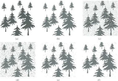
Figure1: Segmentation result of the algorithm for a typical image of synthetic dataset: (a) original image, (b) modified image with medium level of contrast, (c) noisy image of (b) with high additive and multiplicative noise, (d) FCM result, (e) and (f) direct-MC and indirect-MC with automatic seed selection results, respectively.

of both FCM and the proposed algorithms (direct-MC and indirect-MC) is shown. This figure shows that the proposed algorithm reduces the sensitivity of FCM to noise. Moreover, it shows that the indirect MC relation outperforms the direct MC relation. As discussed in Section 3.2, the indirect MC relation has the capability of correcting both FP and FN errors caused by noisy pixels, but the direct MC relation may only correct FP error. The threshold for selection of reference pixels in these experiments was 0.9.

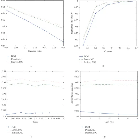
Figure 2 shows the results of our algorithm versus different levels of additive noise, gain, and contrast, sepa-rately. In the depicted diagram, for each factor, the plotted segmentation accuracy is the average resultant accuracy of other factors. As shown in this figure, as the additive noise level (which influences the FCM the most) increases the improvement of the proposed algorithm increases as well. It also shows that the gained improvement by the proposed algorithm in the medium levels of contrast is the most significant. Moreover, the improvement of the proposed algorithm versus different gain levels and different gain types is nearly constant.

In the second experiment, the segmentation of intracra-nial brain tissues (white matter (WM), gray matter (GM),

andcerebrospinal fluid(CSF)) is defined. Assuming 3 clusters

for FCM, the algorithm is applied on the whole slices of brain volume (containing all of these three kinds of tissues) and the intracranial brain mask is extracted from the provided phantom. In this experiment, both Brainweb and IBSR datasets were used.

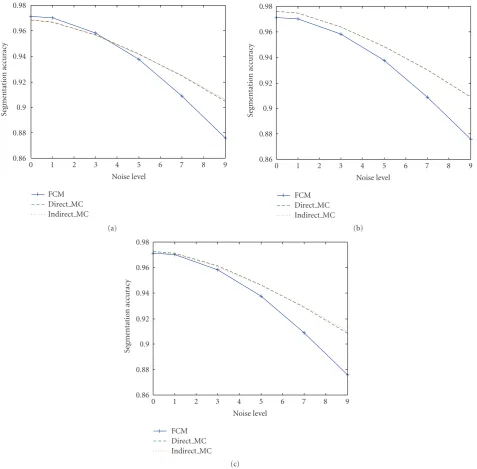
The result of applying the proposed algorithm on diff er-ent datasets of brainweb with different noise levels is shown in Figure 3. In this figure, the segmentation accuracy of FCM, direct MC, and indirect MC algorithms are compared by using automatically selected and optimum seeds. As the segmentation accuracy is measured on the whole brain volume, it can show the behavior of the compared methods solely. This figure clarifies that the integration of FCM and fuzzy connectedness by proposed MC algorithm makes FCM robust in segmentation of noisy images, but at the same time utilization of spatial information might often eliminate details of the image. This effect influenced the detection of small isolated CSF regions (these regions can be seen as small white regions inFigure 4(d)) in brain MRI segmentation which might not be connected to any selected seed pixel. These regions can be better detected using only feature space information (as used in FCM). In noiseless images, where FCM performs well in other regions (WM and GM), the utilization of spatial information is not necessary so the superiority of proposed algorithm is not obvious and the discussed effect in CSF segmentation influences the total segmentation accuracy (as shown in low level noise in Figure 3(a)).

0.84 0.86 0.88 0.9 0.92 0.94 0.96 0.98

Seg

m

entation

ac

cur

acy

0.06 0.08 0.1 0.12 0.14 0.16 0.18 Guassian noise

FCM Direct MC Indirect MC

(a)

0.65 0.7 0.75 0.8 0.85 0.9 0.95 1

Seg

m

entation

ac

cur

acy

0 0.1 0.2 0.3 0.4 0.5 0.6 0.7 Contrast

FCM Direct MC Indirect MC

(b)

0.9 0.905 0.91 0.915 0.92 0.925 0.93 0.935 0.94

Seg

m

entation

ac

cur

acy

0 0.02 0.04 0.06 0.08 0.1 0.12 0.14 0.16 0.18 0.2 Gain

FCM Direct MC Indirect MC

(c)

0.9 0.905 0.91 0.915 0.92 0.925 0.93 0.935 0.94

Seg

m

entation

ac

cur

acy

1 1.5 2 2.5 3 3.5 4

Gain type FCM

Direct MC Indirect MC

(d)

Figure2: Segmentation accuracy versus: (a) noise variance, (b) contrast level, (c) gain factor, (d) gain type for FCM, direct-MC, and indirect-MC.

fi = μo. This kind of specialization can be applied in any

other application in which prior knowledge about existence of such regions is available and they are also detectable after FCM step (In the discussed application the CSF region is detectable because it has the least volume in brain.). Applying this specialization will result inFigure 3(c). Note that in the indirect MC case, the membership degrees are changed by theg(·) function in (7) in the generally proposed algorithm. In order to make the unchanged CSF membership degrees comparable with changed ones of WM and GM in Step 3 of the algorithm, g(·) should be selected as g(x,y) = x×y.

In the ideal seed selection case shown in Figure 3(b), the existence of seeds in any connected component (espe-cially small regions) is guaranteed. Therefore, the discussed problem does not influence the result. This implies that the discussed problem never occurs when error-free seeds are available. The discussed specialization for CSF segmentation is applied in evaluations of the brainweb datasets.

0.86 0.88 0.9 0.92 0.94 0.96 0.98

Seg

m

entation

ac

cur

acy

0 1 2 3 4 5 6 7 8 9

Noise level FCM

Direct MC Indirect MC

(a)

0.86 0.88 0.9 0.92 0.94 0.96 0.98

Seg

m

entation

ac

cur

acy

0 1 2 3 4 5 6 7 8 9

Noise level FCM

Direct MC Indirect MC

(b)

0.86 0.88 0.9 0.92 0.94 0.96 0.98

Seg

m

entation

ac

cur

acy

0 1 2 3 4 5 6 7 8 9

Noise level FCM

Direct MC Indirect MC

(c)

Figure3: Segmentation accuracy of brainweb datasets of different noise levels: (a) with automatic seed selection, (b) with simulated manual seed selection (optimum seeds), (c) with automatic seed selection after specialization of the algorithm for CSF regions.

We would like to mention that brain tissues are complicated and there are long boundaries between them. Therefore, the subjective results of MR image segmentation cannot show the improvement obtained by the proposed algorithm as clear as it can be shown by synthetic images (Figure 1) or by objective evaluations.

As shown inFigure 4, most of the remained segmenta-tion errors are on the border of regions where they cannot be corrected by fuzzy connectedness-based methods. Thus, the results of direct MC and indirect MC methods are similar in this application.

For detailed analysis of the algorithm, the TPVF and FPVF are also measured for default dataset of brainweb

(which contains 3% of noise and 20% of intensity inhomo-geneity). The{TPVF, FPVF}pairs for WM, GM, and CSF are {98.41, 6.53},{93.53, 3.57}, and{94.20, 3.89}, respectively.

(a) (b) (c) (d)

(e) (f) (g) (h)

Figure4: Segmentation result [WM (dark), GM (intermediate brightness), and CSF (bright)] of the proposed algorithm on a typical image of brainweb dataset (slice 80 of the dataset produced by 7% of noise). (a), (b), and (c) T1, T2, and PD images, respectively. (d) Phantom image. (e) FCM result. (f) Direct MC result. (g) Indirect MC result. (h) Error image of direct MC method (white intensity shows the place of error occurrence).

Table 1: Execution time (seconds/image for synthetic and sec-onds/volume for MR images) of proposed algorithms and FCM.

Dataset FCM Direct MC Indirect MC

Synthetic 0.48 1.77 2.46

Brainweb 71.87 83.67 98.45

IBSR 5.65 8.95 12.48

But, these regions are simply detected by the proposed automatic method. As such, the results obtained by using optimum seeds which did not consider any seed in peripheral CSF regions were much better than those of obtained by using automatically selected seeds. In order to eliminate the remained peripheral CSF regions, a postprocessing step was applied by thresholding the CSF membership scene after segmentation algorithms in which the adaptive threshold had been determined using neighborhood pixels of the seeds. After this step, the final segmentation results reached by both direct and indirect MC algorithms were nearly the same. The segmentation results of a typical slice are illustrated in Figure 5. This figure shows that the provided seeds (especially for CSF tissue) and the utilized postprocessing method in the proposed algorithm improve the similarity between segmentation result and reference image but the peripheral CSF regions is not removed completely.

(a) (b)

(c) (d)

Table2: Accuracy results for a dataset of brainweb [co.: coefficient].

Direct MC (optimum seeds) Direct MC, (automatic seeds) Ibrahim et al. [38] Jimenez-Alaniz et al. [39]

Dice co.

CSF 96.71 96.38 — —

WM 96.20 96.04 77.2 —

GM 95.64 95.39 82.8 —

Tanimoto co.

CSF 93.64 93.01 — 87.1

WM 92.68 92.38 — 92.4

GM 91.64 91.18 — 90.0

Table3: Segmentation accuracy (Tanimoto coefficient) and efficiency (average execution time per volume) for IBSR dataset.

Direct MC (optimum seeds) Ibrahim et al. [38] Jimenez-Alaniz et al. [39] Solomon et al. [42] Rivera et al. [43]

Accuracy

CSF 56.87 — 21.0 — —

WM 70.20 66.83 62.8 68.6 74.2

GM 78.50 77.43 59.4 57.5 81.9

Efficiency 8.95 s — — — 3.2 h

In these experiments, we have used Matlab software (except forκFOEMS [18] algorithm that was implemented in C++) on a 1.8-GHz dual core Intel CPU system with 1-GB RAM. The execution time of the proposed algorithm is presented inTable 1 and is compared with FCM runtime. The reported execution time for brainweb is the average runtime on different noise level datasets.

4.3. Comparisons

We have also compared the performance of our proposed algorithm to that of other published reports that have recently been applied on brain tissue segmentation on brainweb or IBSR datasets. These include Ibrahim et al. [38], Jimenez-Alaniz et al. [39], Song et al. [44], Solomon et al. [42], and Rivera et al. [43]. It should be mentioned that as the utilized prior information, preprocessing methods, and postprocessing methods in different reported approaches were not the same, making a fair and meaningful comparison and discussion of segmentation algorithm is not an easy task. Thus, the results given in this section are provided as a reference and some issues should be mentioned before their comparisons. The method in [39] has used prior information in the form of probability maps of voxels and is based on nonparametric density estimation and the mean shift algorithm. In this work, the method is applied on part of the brain volume (131 slices). The methods in [38, 42] are supervised methods and are based on hidden Markov models. In [44] a modified probabilistic neural network is utilized for all head MR image segmentations (both brain and background) and the misclassification rate of 3.41% is reported for brainweb dataset. This method is also a supervised method. In [43] an entropy-controlled quadratic Markov measure field model is used for segmentation purposes. The algorithms reported in [39, 44] and ours segment all intracranial brain tissues but the other methods do not report the result of CSF segmentation. Tables2and

3 list the recent published results on brainweb and IBSR datasets, respectively.

The methods compared in Table 2 have been run on images which have 3% of noise and 20% of intensity inhomogeneity and voxel size of 1 mm3_{. We intended to} include the previous fuzzy connectedness-based segmenta-tion methods in this table, but we did not find any published result for the above-mentioned dataset. In vectorial fuzzy connectedness segmentation [33], true positive volume fraction is reported for brainweb dataset of voxel size of 3 mm3_{(92.6, 95.8, and 94.4 for WM, GM, and CSF, resp.).}

As can be seen from this table, the proposed system which does not use any model and training data outperforms the supervised method described in [38] and the method [39] which utilizes prior information of probability maps. It is worth noticing that the achieved results of our proposed algorithm are based on traditional FCM and thus using improved versions of FCM may lead to better accuracies. Moreover, it was seen that the segmentation error of FCM in the nonnoisy images often occurs in the border of regions. Moreover, we were interested in comparing the execution time of our algorithm with that of other methods used for accuracy comparisons. But, unfortunately their execution times were not reported in their papers except for [43] which used a 3-GHz machine.

5. CONCLUSION

A new image segmentation algorithm was proposed in this paper which is based on a combination of fuzzy connected-ness and fuzzy clustering approaches via a new definition of fuzzy connectedness in membership images. The evaluation of the proposed method (especially based on the FCM algorithm) shows that the proposed algorithm can reduce the sensitivity of fuzzy segmentation algorithms to noise and decreases the false segmentation results when the noise does not occur on region boundaries. This improvement plays an important role especially in medical image applications. The evaluation of the proposed algorithm on real brain MR images clarifies that the new algorithm can utilize the expert knowledge in the form of selected seeds and segments the images as desired by the expert. Also, the proposed method can be integrated with any feature-based fuzzy segmentation method adopted for a specific application. Furthermore, the extension of the proposed membership connectedness method using the scale concept may increase the ability of the algorithm in reducing the sensitivity of feature-based segmentation algorithms to noise. Moreover, the integration of the membership connectedness with a hierarchical fuzzy clustering method that does not require the number of objects will result in a fully automatic segmentation algorithm.

ACKNOWLEDGMENT

This research was in part supported by a grant from ITRC.

REFERENCES

[1] L. A. Zadeh, “Fuzzy sets,”Information and Control, vol. 8, no. 3, pp. 338–353, 1965.

[2] C. K. Gour, D. Laurence, and S. Mahbubur Rahman, “Review of fuzzy image segmentation techniques,” inDesign and Man-agement of Multimedia Information Systems: Opportunities and Challenges, pp. 282–314, IGI Publishing, London, UK, 2001. [3] J. C. Bezdek, J. Keller, R. Krisnapuram, and N. R. Pal,Fuzzy

Models and Algorithms for Pattern Recognition and Image Processing (The Handbooks of Fuzzy Sets), Springer, Berlin, Germany, 2005.

[4] J. V. de Oliveira and W. Pedrycz,Advances in Fuzzy Clustering and Its Applications, John Wiley & Sons, New York, NY, USA, 2007.

[5] J. K. Udupa and S. Samarasekera, “Fuzzy onnectedness and object definition: theory, algorithms, and applications in image segmentation,”Graphical Models and Image Processing, vol. 58, no. 3, pp. 246–261, 1996.

[6] M. Hasanzadeh and S. Kasaei, “Multispectral brain MRI segmentation using genetic fuzzy systems,” inProceedings of the 9th International Symposium on Signal Processing and Its Applications (ISSPA ’07), Sharjah, UAE, February 2007. [7] G. C. Karmakar and L. S. Dooley, “A generic fuzzy rule based

image segmentation algorithm,” Pattern Recognition Letters, vol. 23, no. 10, pp. 1215–1227, 2002.

[8] K. S. Sundareswaran, D. H. Frakes, and A. P. Yoganathan, “Rule-based fuzzy vector median filters for 3D phase contrast MRI segmentation,” inComputational Imaging VI, vol. 6814 ofProceedings of SPIE, pp. 1–14, San Jose, Calif, USA, January 2008.

[9] C. V. Jawahar, P. K. Biswas, and A. K. Ray, “Analysis of fuzzy thresholding schemes,”Pattern Recognition, vol. 33, no. 8, pp. 1339–1349, 2000.

[10] S. K. Pal, A. Ghosh, and B. Uma Shankar, “Segmentation of remotely sensed images with fuzzy thresholding, and quanti-tative evaluation,”International Journal of Remote Sensing, vol. 21, no. 11, pp. 2269–2300, 2000.

[11] J. Kim, W. Cai, S. Eberl, and D. Feng, “Real-time volume rendering visualization of dual-modality PET/CT images with interactive fuzzy thresholding segmentation,”IEEE Transac-tions on Information Technology in Biomedicine, vol. 11, no. 2, pp. 161–169, 2007.

[12] J.-H. Xue, S. Ruan, B. Moretti, M. Revenu, D. Bloyet, and W. Philips, “Fuzzy modeling of knowledge for MRI brain structure segmentation,” inProceedings of IEEE International Conference on Image Processing (ICIP ’00), vol. 1, pp. 617–620, Vancouver, Canada, September 2000.

[13] S. Ruan, B. Moretti, J. Fadili, and D. Bloyet, “Segmentation of magnetic resonance images using fuzzy Markov random fields,” in Proceedings of IEEE International Conference on Image Processing (ICIP ’01), vol. 3, pp. 1051–1054, Thessa-loniki, Greece, October 2001.

[14] L. Xiaodong, Z. Fengqi, and Z. Jun, “Synthetic aperture radar image segmentation based on improved fuzzy Markov random field model,” inProceedings of the 1st International Symposium on Systems and Control in Aerospace and Astro-nautics (ISSCAA ’06), pp. 1205–1208, Harbin, China, January 2006.

[15] M.-E. Algorri and F. Flores-Mangas, “Classification of anatomical structures in MR brain images using fuzzy param-eters,”IEEE Transactions on Biomedical Engineering, vol. 51, no. 9, pp. 1599–1608, 2004.

[16] Z. Xiang, Z. Dazhi, T. Jinwen, and L. Jian, “A hybrid method for 3D segmentation of MRI brain images,” in Proceedings of the 6th International Conference on Signal Processing (ICSP ’02), vol. 1, pp. 608–611, Beijing, China, August 2002. [17] A. Rosenfeld, “Fuzzy geometry: an updated overview,”

Infor-mation Sciences, vol. 110, no. 3-4, pp. 127–133, 1998. [18] J. K. Udupa and P. K. Saha, “Fuzzy connectedness and image

segmentation,” Proceedings of the IEEE, vol. 91, no. 10, pp. 1649–1669, 2003.

[19] A. Rosenfeld, “The fuzzy geometry of image subsets,”Pattern Recognition Letters, vol. 2, no. 5, pp. 311–317, 1984.

[20] S. Dellepiane and F. Fontana, “Extraction of intensity connect-edness for image processing,”Pattern Recognition Letters, vol. 16, no. 3, pp. 313–324, 1995.

[21] A. S. Pednekar and I. A. Kakadiaris, “Image segmentation based on fuzzy connectedness using dynamic weights,”IEEE Transactions on Image Processing, vol. 15, no. 6, pp. 1555–1562, 2006.

[22] X. Fan, J. Yang, Y. Zheng, L. Cheng, and Y. Zhu, “A novel unsupervised segmentation method for MR brain images based on fuzzy methods,” inProceedings of the 1st International Workshop on Computer Vision for Biomedical Image Appli-cations (CVBIA ’05), Y. Liu, T. Jiang, and C. Zhang, Eds., vol. 3765 ofLecture Notes in Computer Science, pp. 160–169, Springer, Beijing, China, October 2005.

[23] D. L. Pham and J. L. Prince, “An adaptive fuzzy C-means algorithm for image segmentation in the presence of intensity inhomogeneities,”Pattern Recognition Letters, vol. 20, no. 1, pp. 57–68, 1999.

[25] M. N. Ahmed, S. M. Yamany, N. Mohamed, A. A. Farag, and T. Moriarty, “A modified fuzzy C-means algorithm for bias field estimation and segmentation of MRI data,”IEEE Transactions on Medical Imaging, vol. 21, no. 3, pp. 193–199, 2002. [26] S. Chen and D. Zhang, “Robust image segmentation using

FCM with spatial constraints based on new kernel-induced distance measure,”IEEE Transactions on Systems, Man, and Cybernetics, Part B, vol. 34, no. 4, pp. 1907–1916, 2004. [27] S. Shen, W. Sandham, M. Granat, and A. Sterr, “MRI fuzzy

segmentation of brain tissue using neighborhood attraction with neural-network optimization,” IEEE Transactions on Information Technology in Biomedicine, vol. 9, no. 3, pp. 459– 467, 2005.

[28] McConnell Brain Imaging Centre,BrainWeb: Simulated Brain DataBase, September 2007, http://www.bic.mni.mcgill.ca/ brainweb.

[29] Center for Morphometric Analysis at Massachusetts General Hospital, July 2007,http://www.cma.mgh.harvard.edu/ibsr. [30] A. Rosenfeld, “Fuzzy digital topology,”Information and

Con-trol, vol. 40, no. 1, pp. 76–87, 1979.

[31] P. K. Saha and J. K. Udupa, “Relative fuzzy connectedness among multiple objects: theory, algorithms, and applications in image segmentation,”Computer Vision and Image Under-standing, vol. 82, no. 1, pp. 42–56, 2001.

[32] P. K. Saha, J. K. Udupa, and D. Odhner, “Scale-based fuzzy connected image segmentation: theory, algorithms, and validation,”Computer Vision and Image Understanding, vol. 77, no. 2, pp. 145–174, 2000.

[33] Y. Zhuge, J. K. Udupa, and P. K. Saha, “Vectorial scale-based fuzzy-connected image segmentation,”Computer Vision and Image Understanding, vol. 101, no. 3, pp. 177–193, 2006. [34] K. C. Ciesielski, J. K. Udupa, P. K. Saha, and Y. Zhuge,

“Iter-ative rel“Iter-ative fuzzy connectedness for multiple objects with multiple seeds,” Computer Vision and Image Understanding, vol. 107, no. 3, pp. 160–182, 2007.

[35] J. C. Bezdek,Pattern Recognition with Fuzzy Objective Function Algorithms, Plenum Press, New York, NY, USA, 1981. [36] R. C. Gonzalez and R. E. Woods, Digital Image Processing,

Prentice Hall, Upper Saddle River, NJ, USA, 2002.

[37] A. K. Jain,Fundamentals of Digital Image Processing, Prentice Hall, Upper Saddle River, NJ, USA, 1989.

[38] M. Ibrahim, N. John, M. Kabuka, and A. Younis, “Hidden Markov models-based 3D MRI brain segmentation,” Image and Vision Computing, vol. 24, no. 10, pp. 1065–1079, 2006. [39] J. R. Jimenez-Alaniz, V. Medina-Banuelos, and O.

Yanez-Suarez, “Data-driven brain MRI segmentation supported on edge confidence and a priori tissue information,” IEEE Transactions on Medical Imaging, vol. 25, no. 1, pp. 74–83, 2006.

[40] V. Grau, A. U. J. Mewes, M. Alca˜niz, R. Kikinis, and S. K. Warfield, “Improved watershed transform for medical image segmentation using prior information,”IEEE Transactions on Medical Imaging, vol. 23, no. 4, pp. 447–458, 2004.

[41] R. O. Duda, P. E. Hart, and D. G. Sork,Pattern Classification, Wiley-Interscience, New York, NY, USA, 2000.

[42] J. Solomon, J. A. Butman, and A. Sood, “Segmentation of brain tumors in 4D MR images using the hidden Markov model,”Computer Methods and Programs in Biomedicine, vol. 84, no. 2-3, pp. 76–85, 2006.

[43] M. Rivera, O. Ocegueda, and J. L. Marroquin, “Entropy-controlled quadratic Markov measure field models for effi -cient image segmentation,”IEEE Transactions on Image Pro-cessing, vol. 16, no. 12, pp. 3047–3057, 2007.