Probability and
Statistics
Third Edition
Murray R. Spiegel, PhD
Former Professor and Chairman of Mathematics
Rensselaer Polytechnic Institute
Hartford Graduate Center
John J. Schiller, PhD
Associate Professor of Mathematics
Temple University
R. Alu Srinivasan, PhD
Professor of Mathematics
Temple University
Schaum’s Outline Series
New York Chicago San Francisco Lisbon London Madrid Mexico City
ISBN: 978-0-07-154426-9 MHID: 0-07-154426-7
The material in this eBook also appears in the print version of this title: ISBN: 978-0-07-154425-2, MHID: 0-07-154425-9.
All trademarks are trademarks of their respective owners. Rather than put a trademark symbol after every occurrence of a trademarked name, we use names in an editorial fashion only, and to the benefit of the trademark owner, with no intention of infringement of the trademark. Where such designations appear in this book, they have been printed with initial caps.
McGraw-Hill eBooks are available at special quantity discounts to use as premiums and sales promotions, or for use in corporate training programs. To contact a representative please e-mail us at [email protected].
TERMS OF USE
This is a copyrighted work and The McGraw-Hill Companies, Inc. (“McGraw-Hill”) and its licensors reserve all rights in and to the work. Use of this work is subject to these terms. Except as permitted under the Copyright Act of 1976 and the right to store and retrieve one copy of the work, you may not decompile, disassemble, reverse engineer, reproduce, modify, create derivative works based upon, transmit, distribute, disseminate, sell, publish or sublicense the work or any part of it without McGraw-Hill’s prior consent. You may use the work for your own noncommercial and personal use; any other use of the work is strict-ly prohibited. Your right to use the work may be terminated if you fail to compstrict-ly with these terms.
iii
Third Edition
In the second edition of Probability and Statistics, which appeared in 2000, the guiding principle was to make
changes in the first edition only where necessary to bring the work in line with the emphasis on topics in con-temporary texts. In addition to refinements throughout the text, a chapter on nonparametric statistics was added to extend the applicability of the text without raising its level. This theme is continued in the third edition in which the book has been reformatted and a chapter on Bayesian methods has been added. In recent years, the Bayesian paradigm has come to enjoy increased popularity and impact in such areas as economics, environmental science, medicine, and finance. Since Bayesian statistical analysis is highly computational, it is gaining even wider ac-ceptance with advances in computer technology. We feel that an introduction to the basic principles of Bayesian data analysis is therefore in order and is consistent with Professor Murray R. Spiegel’s main purpose in writing the original text—to present a modern introduction to probability and statistics using a background of calculus.
J. SCHILLER
R. A. SRINIVASAN
Preface to the
Second Edition
The first edition of Schaum’s Probability and Statistics by Murray R. Spiegel appeared in 1975, and it has gone
through 21 printings since then. Its close cousin, Schaum’s Statisticsby the same author, was described as the
clearest introduction to statistics in print by Gian-Carlo Rota in his book Indiscrete Thoughts. So it was with a
degree of reverence and some caution that we undertook this revision. Our guiding principle was to make changes only where necessary to bring the text in line with the emphasis of topics in contemporary texts. The extensive treatment of sets, standard introductory material in texts of the 1960s and early 1970s, is considerably reduced. The definition of a continuous random variable is now the standard one, and more emphasis is placed on the cu-mulative distribution function since it is a more fundamental concept than the probability density function. Also,
more emphasis is placed on the Pvalues of hypotheses tests, since technology has made it possible to easily
de-termine these values, which provide more specific information than whether or not tests meet a prespecified level of significance. Technology has also made it possible to eliminate logarithmic tables. A chapter on nonpara-metric statistics has been added to extend the applicability of the text without raising its level. Some problem sets have been trimmed, but mostly in cases that called for proofs of theorems for which no hints or help of any kind was given. Overall we believe that the main purpose of the first edition—to present a modern introduction to prob-ability and statistics using a background of calculus—and the features that made the first edition such a great suc-cess have been preserved, and we hope that this edition can serve an even broader range of students.
J. SCHILLER
First Edition
The important and fascinating subject of probability began in the seventeenth century through efforts of such math-ematicians as Fermat and Pascal to answer questions concerning games of chance. It was not until the twentieth century that a rigorous mathematical theory based on axioms, definitions, and theorems was developed. As time progressed, probability theory found its way into many applications, not only in engineering, science, and math-ematics but in fields ranging from actuarial science, agriculture, and business to medicine and psychology. In many instances the applications themselves contributed to the further development of the theory.
The subject of statistics originated much earlier than probability and dealt mainly with the collection, organ-ization, and presentation of data in tables and charts. With the advent of probability it was realized that statistics could be used in drawing valid conclusions and making reasonable decisions on the basis of analysis of data, such as in sampling theory and prediction or forecasting.
The purpose of this book is to present a modern introduction to probability and statistics using a background of calculus. For convenience the book is divided into two parts. The first deals with probability (and by itself can be used to provide an introduction to the subject), while the second deals with statistics.
The book is designed to be used either as a textbook for a formal course in probability and statistics or as a comprehensive supplement to all current standard texts. It should also be of considerable value as a book of ref-erence for research workers or to those interested in the field for self-study. The book can be used for a one-year course, or by a judicious choice of topics, a one-semester course.
I am grateful to the Literary Executor of the late Sir Ronald A. Fisher, F.R.S., to Dr. Frank Yates, F.R.S., and to
Longman Group Ltd., London, for permission to use Table III from their book Statistical Tables for Biological,
Agri-cultural and Medical Research (6th edition, 1974). I also wish to take this opportunity to thank David Beckwith for his outstanding editing and Nicola Monti for his able artwork.
M. R. SPIEGEL
v
Part I
PROBABILITY
1
CHAPTER 1
Basic Probability
3
Random Experiments Sample Spaces Events The Concept of Probability The Axioms
of Probability Some Important Theorems on Probability Assignment of Probabilities
Conditional Probability Theorems on Conditional Probability Independent Events
Bayes’ Theorem or Rule Combinatorial Analysis Fundamental Principle of Counting Tree
Diagrams Permutations Combinations Binomial Coefficients Stirling’s
Approxima-tion to n!
CHAPTER 2
Random Variables and Probability Distributions
34
Random Variables Discrete Probability Distributions Distribution Functions for Random
Variables Distribution Functions for Discrete Random Variables Continuous Random
Vari-ables Graphical Interpretations Joint Distributions Independent Random Variables
Change of Variables Probability Distributions of Functions of Random Variables
Convo-lutions Conditional Distributions Applications to Geometric Probability
CHAPTER 3
Mathematical Expectation
75
Definition of Mathematical Expectation Functions of Random Variables Some Theorems
on Expectation The Variance and Standard Deviation Some Theorems on Variance
Stan-dardized Random Variables Moments Moment Generating Functions Some Theorems
on Moment Generating Functions Characteristic Functions Variance for Joint
Distribu-tions. Covariance Correlation Coefficient Conditional Expectation, Variance, and Moments
Chebyshev’s Inequality Law of Large Numbers Other Measures of Central Tendency
Percentiles Other Measures of Dispersion Skewness and Kurtosis
CHAPTER 4
Special Probability Distributions
108
The Binomial Distribution Some Properties of the Binomial Distribution The Law of
Large Numbers for Bernoulli Trials The Normal Distribution Some Properties of the
Nor-mal Distribution Relation Between Binomial and Normal Distributions The Poisson
Dis-tribution Some Properties of the Poisson Distribution Relation Between the Binomial and
Poisson Distributions Relation Between the Poisson and Normal Distributions The Central
Limit Theorem The Multinomial Distribution The Hypergeometric Distribution The
Uniform Distribution The Cauchy Distribution The Gamma Distribution The Beta
Distribution The Chi-Square Distribution Student’s tDistribution The FDistribution
Relationships Among Chi-Square,t, and FDistributions The Bivariate Normal Distribution
Part II
STATISTICS
151
CHAPTER 5
Sampling Theory
153
Population and Sample. Statistical Inference Sampling With and Without Replacement
Random Samples. Random Numbers Population Parameters Sample Statistics
Sampling Distributions The Sample Mean Sampling Distribution of Means Sampling
Distribution of Proportions Sampling Distribution of Differences and Sums The Sample
Variance Sampling Distribution of Variances Case Where Population Variance Is
Un-known Sampling Distribution of Ratios of Variances Other Statistics Frequency
Distri-butions Relative Frequency Distributions Computation of Mean, Variance, and Moments
for Grouped Data
CHAPTER 6
Estimation Theory
195
Unbiased Estimates and Efficient Estimates Point Estimates and Interval Estimates.
Relia-bility Confidence Interval Estimates of Population Parameters Confidence Intervals for
Means Confidence Intervals for Proportions Confidence Intervals for Differences and
Sums Confidence Intervals for the Variance of a Normal Distribution Confidence Intervals
for Variance Ratios Maximum Likelihood Estimates
CHAPTER 7
Tests of Hypotheses and Significance
213
Statistical Decisions Statistical Hypotheses. Null Hypotheses Tests of Hypotheses and
Significance Type I and Type II Errors Level of Significance Tests Involving the Normal
Distribution One-Tailed and Two-Tailed Tests PValue Special Tests of Significance for
Large Samples Special Tests of Significance for Small Samples Relationship Between
Estimation Theory and Hypothesis Testing Operating Characteristic Curves. Power of a Test
Quality Control Charts Fitting Theoretical Distributions to Sample Frequency Distributions
The Chi-Square Test for Goodness of Fit Contingency Tables Yates’ Correction for
Con-tinuity Coefficient of Contingency
CHAPTER 8
Curve Fitting, Regression, and Correlation
265
Curve Fitting Regression The Method of Least Squares The Least-Squares Line The
Least-Squares Line in Terms of Sample Variances and Covariance The Least-Squares
Parabola Multiple Regression Standard Error of Estimate The Linear Correlation
Coefficient Generalized Correlation Coefficient Rank Correlation Probability
Interpreta-tion of Regression Probability Interpretation of Correlation Sampling Theory of Regression
Sampling Theory of Correlation Correlation and Dependence
CHAPTER 9
Analysis of Variance
314
The Purpose of Analysis of Variance One-Way Classification or One-Factor Experiments
Total Variation. Variation Within Treatments. Variation Between Treatments Shortcut
Meth-ods for Obtaining Variations Linear Mathematical Model for Analysis of Variance
Ex-pected Values of the Variations Distributions of the Variations The FTest for the Null
Hypothesis of Equal Means Analysis of Variance Tables Modifications for Unequal
Num-bers of Observations Two-Way Classification or Two-Factor Experiments Notation for
Two-Factor Experiments Variations for Two-Factor Experiments Analysis of Variance for
CHAPTER 10
Nonparametric Tests
348
Introduction The Sign Test The Mann–Whitney UTest The Kruskal–Wallis HTest
TheHTest Corrected for Ties The Runs Test for Randomness Further Applications of
the Runs Test Spearman’s Rank Correlation
CHAPTER 11
Bayesian Methods
372
Subjective Probability Prior and Posterior Distributions Sampling From a Binomial
Pop-ulation Sampling From a Poisson Population Sampling From a Normal Population with
Known Variance Improper Prior Distributions Conjugate Prior Distributions Bayesian
Point Estimation Bayesian Interval Estimation Bayesian Hypothesis Tests Bayes
Fac-tors Bayesian Predictive Distributions
APPENDIX A
Mathematical Topics
411
Special Sums Euler’s Formulas The Gamma Function The Beta Function Special
Integrals
APPENDIX B
Ordinates
y
of the Standard Normal Curve at
z
413
APPENDIX C
Areas under the Standard Normal Curve from 0 to
z
414
APPENDIX D
Percentile Values
for Student’s
t
Distribution
with Degrees of Freedom
415
APPENDIX E
Percentile Values
for the Chi-Square Distribution
with Degrees of Freedom
416
APPENDIX F
95th and 99th Percentile Values for the
F
Distribution
with ,
Degrees of Freedom
417
APPENDIX G
Values of
e
419
APPENDIX H
Random Numbers
419
SUBJECT INDEX
420
INDEX FOR SOLVED PROBLEMS
423
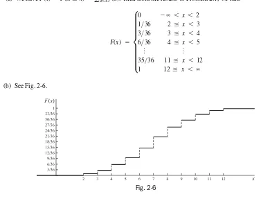
2l
n
2n
1n
x
2
p
3
Basic Probability
Random Experiments
We are all familiar with the importance of experiments in science and engineering. Experimentation is useful to us because we can assume that if we perform certain experiments under very nearly identical conditions, we will arrive at results that are essentially the same. In these circumstances, we are able to control the value of the variables that affect the outcome of the experiment.
However, in some experiments, we are not able to ascertain or control the value of certain variables so that the results will vary from one performance of the experiment to the next even though most of the conditions are
the same. These experiments are described as random. The following are some examples.
EXAMPLE 1.1 If we toss a coin, the result of the experiment is that it will either come up “tails,” symbolized by T(or 0),
or “heads,” symbolized by H(or 1), i.e., one of the elements of the set {H,T} (or {0, 1}).
EXAMPLE 1.2 If we toss a die, the result of the experiment is that it will come up with one of the numbers in the set {1, 2, 3, 4, 5, 6}.
EXAMPLE 1.3 If we toss a coin twice, there are four results possible, as indicated by {HH,HT,TH,T T}, i.e., both heads, heads on first and tails on second, etc.
EXAMPLE 1.4 If we are making bolts with a machine, the result of the experiment is that some may be defective. Thus when a bolt is made, it will be a member of the set {defective, nondefective}.
EXAMPLE 1.5 If an experiment consists of measuring “lifetimes” of electric light bulbs produced by a company, then
the result of the experiment is a time tin hours that lies in some interval—say, 0 t 4000—where we assume that
no bulb lasts more than 4000 hours.
Sample Spaces
A set Sthat consists of all possible outcomes of a random experiment is called a sample space, and each outcome
is called a sample point. Often there will be more than one sample space that can describe outcomes of an
experiment, but there is usually only one that will provide the most information.
EXAMPLE 1.6 If we toss a die, one sample space, or set of all possible outcomes, is given by {1, 2, 3, 4, 5, 6} while another is {odd, even}. It is clear, however, that the latter would not be adequate to determine, for example, whether an outcome is divisible by 3.
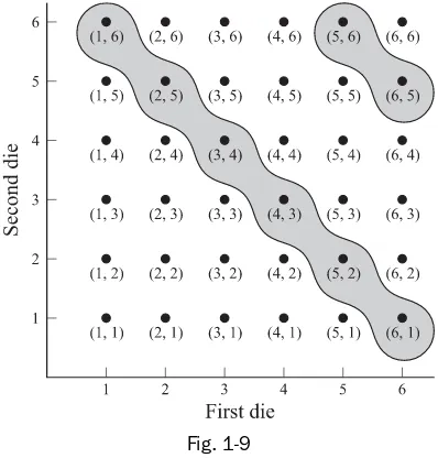
It is often useful to portray a sample space graphically. In such cases it is desirable to use numbers in place of letters whenever possible.
EXAMPLE 1.7 If we toss a coin twice and use 0 to represent tails and 1 to represent heads, the sample space (see Example 1.3) can be portrayed by points as in Fig. 1-1 where, for example, (0, 1) represents tails on first toss and heads
on second toss, i.e.,TH.
If a sample space has a finite number of points, as in Example 1.7, it is called a finite sample space. If it has
as many points as there are natural numbers 1, 2, 3, . . . , it is called a countably infinite sample space. If it has
as many points as there are in some interval on the xaxis, such as 0 x 1, it is called a noncountably infinite
sample space. A sample space that is finite or countably infinite is often called a discrete sample space, while
one that is noncountably infinite is called a nondiscrete sample space.
Events
Aneventis a subset Aof the sample space S, i.e., it is a set of possible outcomes. If the outcome of an
experi-ment is an eleexperi-ment of A, we say that the event A has occurred.An event consisting of a single point of Sis often
called a simpleorelementary event.
EXAMPLE 1.8 If we toss a coin twice, the event that only one head comes up is the subset of the sample space that consists of points (0, 1) and (1, 0), as indicated in Fig. 1-2.
Fig. 1-1
Fig. 1-2
As particular events, we have Sitself, which is the sureorcertain eventsince an element of Smust occur, and
the empty set , which is called the impossible eventbecause an element of cannot occur.
By using set operations on events in S, we can obtain other events in S. For example, if AandBare events, then
1. A Bis the event “either AorBor both.”A Bis called the unionofAandB.
2. A Bis the event “both AandB.”A Bis called the intersectionofAandB.
3. A is the event “not A.”A is called the complementofA.
4. ABA B is the event “Abut not B.” In particular,A SA.
If the sets corresponding to events AandBare disjoint, i.e.,A B , we often say that the events are
mu-tually exclusive. This means that they cannot both occur. We say that a collection of events A1,A2, ,Anis
mu-tually exclusive if every pair in the collection is mumu-tually exclusive.
EXAMPLE 1.9 Referring to the experiment of tossing a coin twice, let Abe the event “at least one head occurs” and
Bthe event “the second toss results in a tail.” Then A{HT,TH,HH},B{HT,TT}, and so we have
AB5TH,HH6 Ar5TT6
A>B5HT6 A<B5HT,TH,HH,TT6S
c
\
d r r
d
r r
d d
< <
The Concept of Probability
In any random experiment there is always uncertainty as to whether a particular event will or will not occur. As
a measure of the chance, or probability, with which we can expect the event to occur, it is convenient to assign
a number between 0 and 1. If we are sure or certain that the event will occur, we say that its probability is 100% or 1, but if we are sure that the event will not occur, we say that its probability is zero. If, for example, the prob-ability is we would say that there is a 25% chance it will occur and a 75% chance that it will not occur.
Equiv-alently, we can say that the oddsagainst its occurrence are 75% to 25%, or 3 to 1.
There are two important procedures by means of which we can estimate the probability of an event.
1. CLASSICAL APPROACH. If an event can occur in hdifferent ways out of a total number of npossible
ways, all of which are equally likely, then the probability of the event is h n.
EXAMPLE 1.10 Suppose we want to know the probability that a head will turn up in a single toss of a coin. Since there are two equally likely ways in which the coin can come up—namely, heads and tails (assuming it does not roll away or stand on its edge)—and of these two ways a head can arise in only one way, we reason that the required probability is
1 2. In arriving at this, we assume that the coin is fair, i.e., not loadedin any way.
2. FREQUENCY APPROACH. If after nrepetitions of an experiment, where nis very large, an event is
observed to occur in hof these, then the probability of the event is h n. This is also called the empirical
probabilityof the event.
EXAMPLE 1.11 If we toss a coin 1000 times and find that it comes up heads 532 times, we estimate the probability
of a head coming up to be 532 1000 0.532.
Both the classical and frequency approaches have serious drawbacks, the first because the words “equally likely” are vague and the second because the “large number” involved is vague. Because of these difficulties,
mathematicians have been led to an axiomatic approachto probability.
The Axioms of Probability
Suppose we have a sample space S. If Sis discrete, all subsets correspond to events and conversely, but if Sis
nondiscrete, only special subsets (called measurable) correspond to events. To each event Ain the class Cof
events, we associate a real number P(A). Then Pis called a probability function, and P(A) the probabilityof the
event A, if the following axioms are satisfied.
Axiom 1 For every event Ain the class C,
P(A) 0 (1)
Axiom 2 For the sure or certain event Sin the class C,
P(S)1 (2)
Axiom 3 For any number of mutually exclusive events A1,A2, , in the class C,
P(A1 A2 )P(A1)P(A2) (3)
In particular, for two mutually exclusive events A1,A2,
P(A1 A2)P(A1)P(A2) (4)
Some Important Theorems on Probability
From the above axioms we can now prove various theorems on probability that are important in further work.
Theorem 1-1 IfA1 A2, then P(A1) P(A2) and P(A2–A1)P(A2)P(A1).
Theorem 1-2 For every event A,
(5)
i.e., a probability is between 0 and 1.
Theorem 1-3 P( ) 0 (6)
i.e., the impossible event has probability zero. \
0P(A)1,
(
<
c c
< <
c
>
> >
> 1
Theorem 1-4 IfA is the complement of A, then
P(A)1P(A) (7)
Theorem 1-5 IfA A1 A2 An, where A1,A2, . . . ,Anare mutually exclusive events, then
P(A)P(A1)P(A2) P(An) (8)
In particular, if AS, the sample space, then
P(A1)P(A2) P(An)1 (9)
Theorem 1-6 IfAandBare any two events, then
P(A B)P(A)P(B) P(A B) (10)
More generally, if A1,A2,A3are any three events, then
P(A1 A2 A3)P(A1)P(A2)P(A3)
P(A1 A2)P(A2 A3)P(A3 A1)
P(A1 A2 A3) (11)
Generalizations to nevents can also be made.
Theorem 1-7 For any events AandB,
P(A)P(A B)P(A B) (12)
Theorem 1-8 If an event A must result in the occurrence of one of the mutually exclusive events
A1,A2, . . . ,An, then
P(A)P(A A1)P(A A2) P(A An) (13)
Assignment of Probabilities
If a sample space Sconsists of a finite number of outcomes a1,a2, ,an, then by Theorem 1-5,
P(A1)P(A2) P(An)1 (14)
whereA1,A2, ,Anare elementary events given by Ai{ai}.
It follows that we can arbitrarily choose any nonnegative numbers for the probabilities of these simple events
as long as (14) is satisfied. In particular, if we assume equal probabilitiesfor all simple events, then
(15)
and if Ais any event made up of hsuch simple events, we have
(16)
This is equivalent to the classical approach to probability given on page 5. We could of course use other pro-cedures for assigning probabilities, such as the frequency approach of page 5.
Assigning probabilities provides a mathematical model, the success of which must be tested by experiment
in much the same manner that theories in physics or other sciences must be tested by experiment.
EXAMPLE 1.12 A single die is tossed once. Find the probability of a 2 or 5 turning up.
The sample space is S{1, 2, 3, 4, 5, 6}. If we assign equal probabilities to the sample points, i.e., if we assume that
the die is fair, then
The event that either 2 or 5 turns up is indicated by 2 5. Therefore,
P(2<5) P(2) P(5) 1
6
1
6
1 3 <
P(1) P(2) cP(6) 1 6
P(A) hn
P(Ak)
1
n, k 1, 2,c, n
c
c
c > c
> >
r > >
> >
> >
> <
<
> <
c
c <c<
<
Conditional Probability
LetAandBbe two events (Fig. 1-3) such that P(A) 0. Denote by P the probability of B given that A
has occurred. Since Ais known to have occurred, it becomes the new sample space replacing the original S.
From this we are led to the definition
(17)
or P(A>B);P(A)P(BuA) (18)
P(BuA);P(A>B)
P(A)
(BuA)
Fig. 1-3
In words, (18) says that the probability that both AandBoccur is equal to the probability that Aoccurs times
the probability that Boccurs given that Ahas occurred. We call P theconditional probabilityofBgiven
A, i.e., the probability that Bwill occur given that Ahas occurred. It is easy to show that conditional probability
satisfies the axioms on page 5.
EXAMPLE 1.13 Find the probability that a single toss of a die will result in a number less than 4 if (a) no other infor-mation is given and (b) it is given that the toss resulted in an odd number.
(a) Let Bdenote the event {less than 4}. Since Bis the union of the events 1, 2, or 3 turning up, we see by Theorem 1-5 that
assuming equal probabilities for the sample points.
(b) Letting Abe the event {odd number}, we see that Then
Hence, the added knowledge that the toss results in an odd number raises the probability from 1 2 to 2 3.
Theorems on Conditional Probability
Theorem 1-9 For any three events A1,A2,A3, we haveP(A1 A2 A3)P(A1)P(A2 A1)P(A3 A1 A2) (19)
In words, the probability that A1andA2andA3all occur is equal to the probability that A1occurs times the
probability that A2occurs given that A1has occurred times the probability that A3occurs given that both A1andA2
have occurred. The result is easily generalized to nevents.
Theorem 1-10 If an event Amust result in one of the mutually exclusive events A1,A2, ,An, then
P(A)P(A1)P(A A1)P(A2)P(A A2) P(An)P(A An) (20)
Independent Events
IfP(B A)P(B), i.e., the probability of Boccurring is not affected by the occurrence or non-occurrence of A,
then we say that AandBareindependent events. This is equivalent to
P(A B)P(A)P(B) (21)
as seen from (18). Conversely, if (21) holds, then AandBare independent.
> u
u
c
u u
c >
u u
> >
> > P(BuA)P(A>B)
P(A) 1>3
1>2
2 3
P(A)36 1
2. Also P(A> B)26 13.
P(B)P(1)P(2)P(3)1
6
1
6
1
6
1 2
We say that three events A1,A2,A3areindependentif they are pairwise independent:
P(Aj Ak)P(Aj)P(Ak) j k where j,k1, 2, 3 (22)
and P(A1 A2 A3)P(A1)P(A2)P(A3) (23)
Note that neither (22) nor (23) is by itself sufficient. Independence of more than three events is easily defined.
Bayes’ Theorem or Rule
Suppose that A1,A2, ,Anare mutually exclusive events whose union is the sample space S, i.e., one of the
events must occur. Then if Ais any event, we have the following important theorem:
Theorem 1-11(Bayes’ Rule):
(24)
This enables us to find the probabilities of the various events A1,A2, ,Anthat can cause Ato occur. For this
reason Bayes’ theorem is often referred to as a theorem on the probability of causes.
Combinatorial Analysis
In many cases the number of sample points in a sample space is not very large, and so direct enumeration or counting of sample points needed to obtain probabilities is not difficult. However, problems arise where direct
counting becomes a practical impossibility. In such cases use is made of combinatorial analysis, which could also
be called a sophisticated way of counting.
Fundamental Principle of Counting: Tree Diagrams
If one thing can be accomplished in n1different ways and after this a second thing can be accomplished in n2
dif-ferent ways, . . . , and finally a kth thing can be accomplished in nkdifferent ways, then all kthings can be
ac-complished in the specified order in n1n2 nkdifferent ways.
EXAMPLE 1.14 If a man has 2 shirts and 4 ties, then he has 2 4 8 ways of choosing a shirt and then a tie.
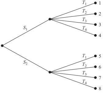
A diagram, called a tree diagrambecause of its appearance (Fig. 1-4), is often used in connection with the
above principle.
EXAMPLE 1.15 Letting the shirts be represented by S1,S2and the ties by T1,T2,T3,T4, the various ways of choosing a shirt and then a tie are indicated in the tree diagram of Fig. 1-4.
?
c
c
P(AkuA)
P(Ak)P(AuAk)
a
n
j1
P(Aj)P(AuAj)
c
> >
2 >
Permutations
Suppose that we are given ndistinct objects and wish to arrange rof these objects in a line. Since there are n
ways of choosing the 1st object, and after this is done,n 1 ways of choosing the 2nd object, . . . , and finally
n r1 ways of choosing the rth object, it follows by the fundamental principle of counting that the number
of different arrangements, or permutationsas they are often called, is given by
nPrn(n 1)(n 2) (n r1) (25)
where it is noted that the product has rfactors. We call nPrthenumber of permutations of n objects taken r at a time.
In the particular case where rn, (25) becomes
nPnn(n1)(n2) 1 n! (26)
which is called n factorial. We can write (25) in terms of factorials as
(27)
Ifrn, we see that (27) and (26) agree only if we have 0! 1, and we shall actually take this as the definition of 0!.
EXAMPLE 1.16 The number of different arrangements, or permutations, consisting of 3 letters each that can be formed
from the 7 letters A,B,C,D,E,F,Gis
Suppose that a set consists of nobjects of which n1are of one type (i.e., indistinguishable from each other),
n2are of a second type, . . . ,nkare of a kth type. Here, of course,nn1n2 nk. Then the number of
different permutations of the objects is
(28)
See Problem 1.25.
EXAMPLE 1.17 The number of different permutations of the 11 letters of the word M I S S I S S I P P I, which con-sists of 1 M, 4 I’s, 4 S’s, and 2 P’s, is
Combinations
In a permutation we are interested in the order of arrangement of the objects. For example,abcis a different
per-mutation from bca. In many problems, however, we are interested only in selecting or choosing objects without
regard to order. Such selections are called combinations. For example,abcandbcaare the same combination.
The total number of combinations of robjects selected from n(also called the combinations of n things taken
r at a time) is denoted by nCror We have (see Problem 1.27)
(29)
It can also be written
(30)
It is easy to show that
(31) ¢n
r≤ ¢ n
n r≤ or nCrnCnr
¢n
r≤
n(n 1) c(n r1)
r!
nPr
r! ¢n
r≤ nCr n!
r!(n r)! an
rb.
11!
1!4!4!2!34,650
nPn1,n2,c,nk
n!
n1!n2!cnk!
c
7P3 7!
4!7?6?5210
nPr
n!
(n r)!
EXAMPLE 1.18 The number of ways in which 3 cards can be chosen or selected from a total of 8 different cards is
Binomial Coefficient
The numbers (29) are often called binomial coefficientsbecause they arise in the binomial expansion
(32)
They have many interesting properties.
EXAMPLE 1.19
Stirling’s Approximation to n!
Whennis large, a direct evaluation of n! may be impractical. In such cases use can be made of the approximate
formula
(33)
wheree2.71828 . . . , which is the base of natural logarithms. The symbol in (33) means that the ratio of
the left side to the right side approaches 1 as n .
Computing technology has largely eclipsed the value of Stirling’s formula for numerical computations, but the approximation remains valuable for theoretical estimates (see Appendix A).
SOLVED PROBLEMS
Random experiments, sample spaces, and events
1.1.A card is drawn at random from an ordinary deck of 52 playing cards. Describe the sample space if
consid-eration of suits (a) is not, (b) is, taken into account.
(a) If we do not take into account the suits, the sample space consists of ace, two, . . . , ten, jack, queen, king, and it can be indicated as {1, 2, . . . , 13}.
(b) If we do take into account the suits, the sample space consists of ace of hearts, spades, diamonds, and clubs; . . . ; king of hearts, spades, diamonds, and clubs. Denoting hearts, spades, diamonds, and clubs, respectively, by 1, 2, 3, 4, for example, we can indicate a jack of spades by (11, 2). The sample space then consists of the 52 points shown in Fig. 1-5.
`
S
,
n!, 22pn nnen
x44x3y6x2y24xy3y4
(xy)4x4 ¢4
1≤x
3y ¢4
2≤x
2y2 ¢4
3≤xy
3 ¢4
4≤y
4
(xy)nxn ¢n
1≤x
n1y ¢n
2≤x
n2y2c ¢n
n≤y
n
8C3¢ 8
3≤
8?7?6
3! 56
1.2.Referring to the experiment of Problem 1.1, let Abe the event {king is drawn} or simply {king} and Bthe
event {club is drawn} or simply {club}. Describe the events (a) A B, (b) A B, (c) A B, (d) A B,
(e)A B, (f ) A B, (g) (A B) (A B).
(a) A B{either king or club (or both, i.e., king of clubs)}.
(b) A B{both king and club} {king of clubs}.
(c) Since B{club},B {not club} {heart, diamond, spade}.
Then A B {king or heart or diamond or spade}.
(d ) A B {not king or not club} {not king of clubs} {any card but king of clubs}.
This can also be seen by noting that A B (A B) and using (b).
(e) A B{king but not club}.
This is the same as A B {king and not club}.
(f ) A B {not king and not “not club”} {not king and club} {any club except king}.
This can also be seen by noting that A B A (B) A B.
(g) (A B) (A B){(king and club) or (king and not club)} {king}.
This can also be seen by noting that (A B) (A B)A.
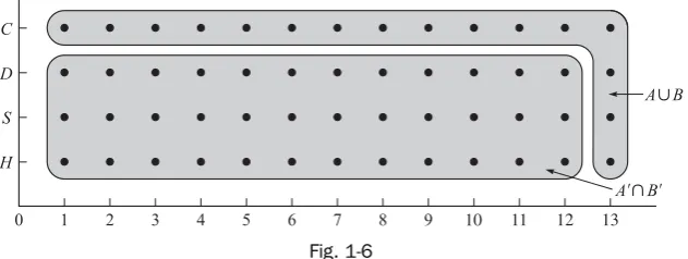
1.3.Use Fig. 1-5 to describe the events (a) A B, (b) A B.
The required events are indicated in Fig. 1-6. In a similar manner, all the events of Problem 1.2 can also be
indi-cated by such diagrams. It should be observed from Fig. 1-6 that Ar>Bris the complement of A<B.
r
>
r
<
r
> < >
r
> < >
>
r r r
>
r r r r
r
r
>
r
>
r
<
r r
<
r
r
<
r
> <
r > < > r
r
r < r r < >
<
Fig. 1-6
Theorems on probability
1.4.Prove (a) Theorem 1-1, (b) Theorem 1-2, (c) Theorem 1-3, page 5.
(a) We have A2A1 (A2 A1) where A1andA2 A1are mutually exclusive. Then by Axiom 3, page 5:
P(A2)P(A1)P(A2 A1)
so that P(A2 A1)P(A2) P(A1)
SinceP(A2 A1) 0 by Axiom 1, page 5, it also follows that P(A2) P(A1).
(b) We already know that P(A) 0 by Axiom 1. To prove that P(A) 1, we first note that A S. Therefore,
by Theorem 1-1 [part (a)] and Axiom 2,
P(A) P(S)1
(c) We have SS . Since S , it follows from Axiom 3 that
P(S)P(S)P( )\ or P( ) \ 0
\ > \ \
<
(
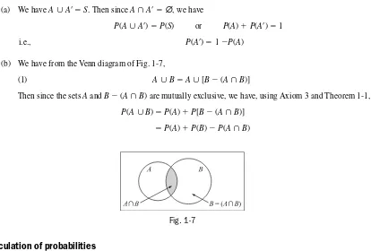
1.5. Prove (a) Theorem 1-4, (b) Theorem 1-6.
(a) We have A A S. Then since A A , we have
P(A A)P(S) or P(A)P(A)1
i.e., P(A)1P(A)
(b) We have from the Venn diagram of Fig. 1-7,
(1) A BA [B (A B)]
Then since the sets AandB (A B) are mutually exclusive, we have, using Axiom 3 and Theorem 1-1,
P(A B)P(A)P[B (A B)] P(A)P(B) P(A>B)
> <
>
> <
<
r
r r
<
\
r
>
r
<
Fig. 1-7
Calculation of probabilities
1.6.A card is drawn at random from an ordinary deck of 52 playing cards. Find the probability that it is (a) an
ace, (b) a jack of hearts, (c) a three of clubs or a six of diamonds, (d ) a heart, (e) any suit except hearts, (f) a ten or a spade, (g) neither a four nor a club.
Let us use for brevity H,S,D,Cto indicate heart, spade, diamond, club, respectively, and 1, 2 13 for
ace, two, , king. Then 3 Hmeans three of hearts, while 3 Hmeans three or heart. Let us use the
sample space of Problem 1.1(b), assigning equal probabilities of 1 52 to each sample point. For example,
P(6 C)1 52.
(a)
This could also have been achieved from the sample space of Problem 1.1(a) where each sample point, in particular ace, has probability 1 13. It could also have been arrived at by simply reasoning that there are 13 numbers and so each has probability 1 13 of being drawn.
(b)
(c)
(d )
This could also have been arrived at by noting that there are four suits and each has equal probability of
being drawn.
(e) using part (d) and Theorem 1-4, page 6.
(f ) Since 10 and Sare not mutually exclusive, we have, from Theorem 1-6,
(g) The probability of neither four nor club can be denoted by P(4r>Cr). But 4r>Cr(4<C) .r
P(10<S)P(10)P(S)P(10 > S) 1
13
1
4
1
52
4 13 P(Hr)1P(H)11
4
3 4
1>2 P(H)P(1> H or 2 >H or c13 > H) 1
52
1
52 c
1
52
13
52
1 4 P(3>C or 6 > D)P(3> C)P(6 > D) 1
52
1
52
1 26 P(11>H)521
> >
521 521 521 521 131
P(1>H)P(1>S)P(1>D)P(1>C) P(1)P(1>H or 1 >S or 1 >D or 1 >C)
>
> >
< >
Therefore,
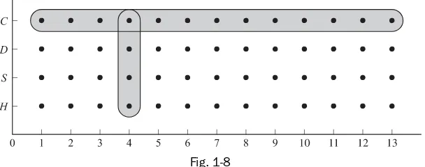
We could also get this by noting that the diagram favorable to this event is the complement of the event
shown circled in Fig. 1-8. Since this complement has 52 1636 sample points in it and each sample point
is assigned probability 1 52, the required probability is 36 52 > > 9 13.>
1 B 1
13
1
4
1
52R
9 13
1 [P(4) P(C)P(4>C)]
P(4r>Cr)P[(4<C)r] 1 P(4<C)
Fig. 1-8
1.7.A ball is drawn at random from a box containing 6 red balls, 4 white balls, and 5 blue balls. Determine the
probability that it is (a) red, (b) white, (c) blue, (d) not red, (e) red or white.
(a) Method 1
LetR,W, and Bdenote the events of drawing a red ball, white ball, and blue ball, respectively. Then
Method 2
Our sample space consists of 6 4515 sample points. Then if we assign equal probabilities 1 15 to>
P(R)total ways of choosing a ballways of choosing a red ball 6465156 25
each sample point, we see that P(R)6 15 2 5, since there are 6 sample points corresponding to “red ball.”
(b)
(c)
(d) by part (a).
(e) Method 1
This can also be worked using the sample space as in part (a).
Method 2
by part (c).
Method 3
Since events RandWare mutually exclusive, it follows from (4), page 5, that
P(R<W)P(R)P(W)2
5
4
15
2 3 P(R<W)P(Br)1P(B)113 23
6644 5101523
P(red or white)P(R<W)ways of choosing a red or white ball total ways of choosing a ball P(not red)P(Rr)1P(R)12535
P(B)6545 155 13 P(W)6445 154
Conditional probability and independent events
1.8.A fair die is tossed twice. Find the probability of getting a 4, 5, or 6 on the first toss and a 1, 2, 3, or 4 on
the second toss.
LetA1be the event “4, 5, or 6 on first toss,” and A2be the event “1, 2, 3, or 4 on second toss.” Then we are
looking for P(A1 A2).
Method 1
We have used here the fact that the result of the second toss is independentof the first so that P(A2uA1)P(A2).
P(A1> A2)P(A1)P(A2uA1)P(A1)P(A2)¢ 3
6≤ ¢
4
6≤
1 3
>
Fig. 1-9
If we let Abe the event “7 or 11,” then Ais indicated by the circled portion in Fig. 1-9. Since 8 points are
included, we have P(A)8 36 2 9. It follows that the probability of no 7 or 11 is given by
P(Ar)1P(A)12
9
7 9 >
>
Also we have used P(A1)3 6 (since 4, 5, or 6 are 3 out of 6 equally likely possibilities) and P(A2)4 6 (since
1, 2, 3, or 4 are 4 out of 6 equally likely possibilities).
Method 2
Each of the 6 ways in which a die can fall on the first toss can be associated with each of the 6 ways in which it
can fall on the second toss, a total of 6 6 36 ways, all equally likely.
Each of the 3 ways in which A1can occur can be associated with each of the 4 ways in which A2can occur to
give 3 4 12 ways in which both A1andA2can occur. Then
This shows directly that A1andA2are independent since
1.9.Find the probability of not getting a 7 or 11 total on either of two tosses of a pair of fair dice.
The sample space for each toss of the dice is shown in Fig. 1-9. For example, (5, 2) means that 5 comes up on the first die and 2 on the second. Since the dice are fair and there are 36 sample points, we assign probability
1 36 to each.>
P(A1>A2) 1
3 ¢
3
6≤ ¢
4
6≤ P(A1)P(A2)
P(A1>A2) 12
36
1 3
?
?
Using subscripts 1, 2 to denote 1st and 2nd tosses of the dice, we see that the probability of no 7 or 11 on either the first or second tosses is given by
using the fact that the tosses are independent.
1.10. Two cards are drawn from a well-shuffled ordinary deck of 52 cards. Find the probability that they are both
aces if the first card is (a) replaced, (b) not replaced.
Method 1
LetA1event “ace on first draw” and A2event “ace on second draw.” Then we are looking for P(A1 A2)
P(A1)P(A2 A1).
(a) Since for the first drawing there are 4 aces in 52 cards,P(A1)4 52. Also, if the card is replaced for the>
u >
P(A1r)P(Ar2uAr1)P(Ar1)P(Ar2) ¢ 7
9≤ ¢
7
9≤
49 81,
second drawing, then P(A2 A1)4 52, since there are also 4 aces out of 52 cards for the second drawing.
Then
(b) As in part (a),P(A1)4 52. However, if an ace occurs on the first drawing, there will be only 3 aces left in>
P(A1>A2)P(A1)P(A2uA1)¢ 4
52≤ ¢
4
52≤
1 169 >
u
the remaining 51 cards, so that P(A2 A1)3 51. Then
Method 2
(a) The first card can be drawn in any one of 52 ways, and since there is replacement, the second card can also be drawn in any one of 52 ways. Then both cards can be drawn in (52)(52) ways, all equally likely.
In such a case there are 4 ways of choosing an ace on the first draw and 4 ways of choosing an ace on the second draw so that the number of ways of choosing aces on the first and second draws is (4)(4). Then the required probability is
(b) The first card can be drawn in any one of 52 ways, and since there is no replacement, the second card can be drawn in any one of 51 ways. Then both cards can be drawn in (52)(51) ways, all equally likely.
In such a case there are 4 ways of choosing an ace on the first draw and 3 ways of choosing an ace on the second draw so that the number of ways of choosing aces on the first and second draws is (4)(3). Then the required probability is
1.11. Three balls are drawn successively from the box of Problem 1.7. Find the probability that they are drawn
in the order red, white, and blue if each ball is (a) replaced, (b) not replaced.
LetR1event “red on first draw,”W2event “white on second draw,”B3event “blue on third draw.” We
requireP(R1 W2 B3).
(a) If each ball is replaced, then the events are independent and
¢6645≤ ¢6445≤ ¢6545≤2258 P(R1)P(W2)P(B3)
P(R1>W2>B3)P(R1)P(W2uR1)P(B3uR2>W2)
> >
(4)(3)
(52)(51)
1 221 (4)(4)
(52)(52)
1 169 P(A1>A2)P(A1)P(A2
Z
A1)¢4
52≤ ¢
3
51≤
1 221 >
(b) If each ball is not replaced, then the events are dependent and
1.12. Find the probability of a 4 turning up at least once in two tosses of a fair die.
LetA1event “4 on first toss” and A2event “4 on second toss.” Then
A1 A2event “4 on first toss or 4 on second toss or both”
event “at least one 4 turns up,”
and we require P(A1 A2).
Method 1
Events A1andA2are not mutually exclusive, but they are independent. Hence, by (10) and (21),
Method 2
P(at least one 4 comes up) P(no 4 comes up) 1 Then P(at least one 4 comes up) 1 P(no 4 comes up)
1 P(no 4 on 1st toss and no 4 on 2nd toss)
Method 3
Total number of equally likely ways in which both dice can fall 6 6 36.
Also Number of ways in which A1occurs but not A25
Number of ways in which A2occurs but not A15
Number of ways in which both A1andA2occur1
Then the number of ways in which at least one of the events A1orA2occurs55111. Therefore,
P(A1 A2)11 36.
1.13. One bag contains 4 white balls and 2 black balls; another contains 3 white balls and 5 black balls. If one
ball is drawn from each bag, find the probability that (a) both are white, (b) both are black, (c) one is white and one is black.
LetW1event “white ball from first bag,”W2event “white ball from second bag.”
(a)
(b)
(c) The required probability is
1.14. Prove Theorem 1-10, page 7.
We prove the theorem for the case n2. Extensions to larger values of nare easily made. If event Amust
result in one of the two mutually exclusive events A1,A2, then
A(A>A1)<(A>A2)
1P(W1>W2)P(W1r>Wr2)1
1
4
5
24
13 24 P(Wr1>Wr2)P(W1r)P(Wr2uW1r)P(Wr1)P(Wr2) ¢
2
42≤ ¢
5
35≤
5 24 P(W1>W2)P(W1)P(W2uW1)P(W1)P(W2)¢
4
42≤ ¢
3
35≤
1 4 >
<
?
1¢56≤ ¢56≤ 1136
1P(A1r>Ar2)1P(Ar1)P(Ar2)
16 16 ¢16≤ ¢16≤ 1136 P(A1)P(A2)P(A1)P(A2) P(A1< A2)P(A1)P(A2)P(A1>A2)
< <
ButA A1andA A2are mutually exclusive since A1andA2are. Therefore, by Axiom 3,
P(A)P(A A1)P(A A2)
P(A1)P(A A1)P(A2)P(A A2)
using (18), page 7.
1.15. BoxIcontains 3 red and 2 blue marbles while Box IIcontains 2 red and 8 blue marbles. A fair coin is
tossed. If the coin turns up heads, a marble is chosen from Box I; if it turns up tails, a marble is chosen
from Box II. Find the probability that a red marble is chosen.
LetRdenote the event “a red marble is chosen” while IandIIdenote the events that Box Iand Box IIare
chosen, respectively. Since a red marble can result by choosing either Box IorII, we can use the results of
Problem 1.14 with AR,A1I,A2II. Therefore, the probability of choosing a red marble is
Bayes’ theorem
1.16. Prove Bayes’ theorem (Theorem 1-11, page 8).
SinceAresults in one of the mutually exclusive events A1,A2, ,An, we have by Theorem 1-10
(Problem 1.14),
Therefore,
1.17. Suppose in Problem 1.15 that the one who tosses the coin does not reveal whether it has turned up heads
or tails (so that the box from which a marble was chosen is not revealed) but does reveal that a red
mar-ble was chosen. What is the probability that Box Iwas chosen (i.e., the coin turned up heads)?
Let us use the same terminology as in Problem 1.15, i.e.,AR,A1I,A2II. We seek the probability that Box
Iwas chosen given that a red marble is known to have been chosen. Using Bayes’ rule with n2, this probability
is given by
Combinational analysis, counting, and tree diagrams
1.18. A committee of 3 members is to be formed consisting of one representative each from labor, management,
and the public. If there are 3 possible representatives from labor, 2 from management, and 4 from the pub-lic, determine how many different committees can be formed using (a) the fundamental principle of count-ing and (b) a tree diagram.
(a) We can choose a labor representative in 3 different ways, and after this a management representative in 2
different ways. Then there are 3 2 6 different ways of choosing a labor and management representative.
With each of these ways we can choose a public representative in 4 different ways. Therefore, the number
of different committees that can be formed is 3?2?4 24.
?
P(IuR) P(I)P(RuI)
P(I)P(RuI)P(II)P(RuII)
¢12≤ ¢33 2≤
¢12≤ ¢33 2≤ ¢12≤ ¢22 8≤ 34 P(AkuA)
P(Ak>A)
P(A)
P(Ak)P(AuAk)
a
n
j1
P(Aj)P(AuAj)
P(A)P(A1)P(AuA1) cP(An)P(AuAn) a n
j1
P(Aj)P(AuAj)
c
P(R)P(I)P(RuI)P(II)P(RuII) ¢12≤ ¢33 2≤ ¢12≤ ¢22 8≤ 25
u u
> >
(b) Denote the 3 labor representatives by L1,L2,L3; the management representatives by M1,M2; and the public
representatives by P1,P2,P3,P4. Then the tree diagram of Fig. 1-10 shows that there are 24 different
committees in all. From this tree diagram we can list all these different committees, e.g.,L1M1P1,L1M1P2, etc.
Fig. 1-10
Permutations
1.19. In how many ways can 5 differently colored marbles be arranged in a row?
We must arrange the 5 marbles in 5 positions thus:. The first position can be occupied by any one of
5 marbles, i.e., there are 5 ways of filling the first position. When this has been done, there are 4 ways of filling the second position. Then there are 3 ways of filling the third position, 2 ways of filling the fourth position, and finally only 1 way of filling the last position. Therefore:
Number of arrangements of 5 marbles in a row 5 4 3 2 l 5!120
In general,
Number of arrangements of ndifferent objects in a row n(n l)(n 2) 1 n!
This is also called the number of permutations of n different objects taken n at a time and is denoted by nPn.
1.20. In how many ways can 10 people be seated on a bench if only 4 seats are available?
The first seat can be filled in any one of 10 ways, and when this has been done, there are 9 ways of filling the second seat, 8 ways of filling the third seat, and 7 ways of filling the fourth seat. Therefore:
Number of arrangements of 10 people taken 4 at a time 10 9 8 7 5040
In general,
Number of arrangements of ndifferent objects taken rat a time n(n 1) (n r1)
This is also called the number of permutations of n different objects taken r at a time and is denoted by nPr.
Note that when rn,nPnn! as in Problem 1.19.
c
? ? ?
c
1.21. Evaluate (a) 8P3, (b) 6P4, (c) l5P1, (d) 3P3.
(a) 8P38 7 6 336 (b) 6P46 5 4 3 360 (c) 15P115 (d) 3P33 2 1 6
1.22. It is required to seat 5 men and 4 women in a row so that the women occupy the even places. How many
such arrangements are possible?
The men may be seated in 5P5ways, and the women in 4P4ways. Each arrangement of the men may be
associated with each arrangement of the women. Hence,
Number of arrangements 5P5 4P45! 4! (120)(24)2880
1.23. How many 4-digit numbers can be formed with the 10 digits 0, 1, 2, 3, . . . , 9 if (a) repetitions are allowed,
(b) repetitions are not allowed, (c) the last digit must be zero and repetitions are not allowed?
(a) The first digit can be any one of 9 (since 0 is not allowed). The second, third, and fourth digits can be any
one of 10. Then 9 10 10 10 9000 numbers can be formed.
(b) The first digit can be any one of 9 (any one but 0).
The second digit can be any one of 9 (any but that used for the first digit).
The third digit can be any one of 8 (any but those used for the first two digits).
The fourth digit can be any one of 7 (any but those used for the first three digits).
Then 9 9 8 7 4536 numbers can be formed.
Another method
The first digit can be any one of 9, and the remaining three can be chosen in 9P3ways. Then 9 9P3
9 9 8 7 4536 numbers can be formed.
(c) The first digit can be chosen in 9 ways, the second in 8 ways, and the third in 7 ways. Then 9 8 7 504
numbers can be formed.
Another method
The first digit can be chosen in 9 ways, and the next two digits in 8P2ways. Then 9 8P29 8 7
504 numbers can be formed.
1.24. Four different mathematics books, six different physics books, and two different chemistry books are to
be arranged on a shelf. How many different arrangements are possible if (a) the books in each particular subject must all stand together, (b) only the mathematics books must stand together?
(a) The mathematics books can be arranged among themselves in4P44! ways, the physics books in 6P66!
ways, the chemistry books in 2P22! ways, and the three groups in 3P33! ways. Therefore,
Number of arrangements 4!6!2!3!207,360.
(b) Consider the four mathematics books as one big book. Then we have 9 books which can be arranged in
9P99! ways. In all of these ways the mathematics books are together. But the mathematics books can be
arranged among themselves in 4P44! ways. Hence,
Number of arrangements 9!4!8,709,120
1.25. Five red marbles, two white marbles, and three blue marbles are arranged in a row. If all the marbles of
the same color are not distinguishable from each other, how many different arrangements are possible?
Assume that there are Ndifferent arrangements. Multiplying Nby the numbers of ways of arranging (a) the five
red marbles among themselves, (b) the two white marbles among themselves, and (c) the three blue marbles
among themselves (i.e., multiplying Nby 5!2!3!), we obtain the number of ways of arranging the 10 marbles if
they were all distinguishable, i.e., 10!.
Then (5!2!3!)N10! and N10! (5!2!3!)
In general, the number of different arrangements of nobjects of which n1are alike,n2are alike, . . . ,nkare
alike is where n1n2cnkn.
n! n1!n2!cnk!
>
? ? ?
? ? ?
?
? ?
? ? ?
? ? ?
?
? ? ?
? ? ?
1.26. In how many ways can 7 people be seated at a round table if (a) they can sit anywhere, (b) 2 particular peo-ple must not sit next to each other?
(a) Let 1 of them be seated anywhere. Then the remaining 6 people can be seated in 6! 720 ways, which is
the total number of ways of arranging the 7 people in a circle.
(b) Consider the 2 particular people as 1 person. Then there are 6 people altogether and they can be arranged in 5! ways. But the 2 people considered as 1 can be arranged in 2! ways. Therefore, the number of ways of
arranging 7 people at a round table with 2 particular people sitting together 5!2!240.
Then using (a), the total number of ways in which 7 people can be seated at a round table so that the 2
particular people do not sit together 730240480 ways.
Combinations
1.27. In how many ways can 10 objects be split into two groups containing 4 and 6 objects, respectively?
This is the same as the number of arrangements of 10 objects of which 4 objects are alike and 6 other objects are alike. By Problem 1.25, this is
The problem is equivalent to finding the number of selections of 4 out of 10 objects (or 6 out of 10 objects), the
order of selection being immaterial. In general, the number of selections of rout of nobjects, called the number
10!
4!6!
10?9?8?7
4! 210.
of combinations of n things taken r at a time,is denoted by nCror and is given by
1.28. Evaluate (a) 7C4, (b) 6C5, (c) 4C4.
(a)
(b)
(c) 4C4is the number of selections of 4 objects taken 4 at a time, and there is only one such selection. Then 4C41.
Note that formally
if we define0!1.
1.29. In how many ways can a committee of 5 people be chosen out of 9 people?
1.30. Out of 5 mathematicians and 7 physicists, a committee consisting of 2 mathematicians and 3 physicists
is to be formed. In how many ways can this be done if (a) any mathematician and any physicist can be in-cluded, (b) one particular physicist must be on the committee, (c) two particular mathematicians cannot be on the committee?
(a) 2 mathematicians out of 5 can be selected in 5C2ways.
3 physicists out of 7 can be selected in 7C3ways.
Total number of possible selections 5C2 7C310 35 350
(b) 2 mathematicians out of 5 can be selected in 5C2ways.
2 physicists out of 6 can be selected in 6C2ways.
Total number of possible selections 5C2 6C210 15 150
(c) 2 mathematicians out of 3 can be selected in 3C2ways.
3 physicists out of 7 can be selected in 7C3ways.
Total number of possible selections 3C2? 7C33?35 105
? ?
? ?
¢9
5≤ 9C5
9!
5!4!
9 ?8?7?6 ?5
5! 126
4C4 4!
4!0!1
6C5 6!
5!1!
6?5?4?3?2
5! 6, or 6C56C16.
7C4 7!
4!3!
7?6?5?4
4!
7?6?5
3?2?135.
nCr ¢
n r≤
n! r!(nr)!
n(n1)c(nr1)
r!
nPr
r!
1.31. How many different salads can be made from lettuce, escarole, endive, watercress, and chicory?
Each green can be dealt with in 2 ways, as it can be chosen or not chosen. Since each of the 2 ways of dealing with a green is associated with 2 ways of dealing with each of the other greens, the number of ways of dealing
with the 5 greens 25ways. But 25ways includes the case in which no greens is chosen. Hence,
Number of salads 25131
Another method
One can select either 1 out of 5 greens, 2 out of 5 greens, . . . , 5 out of 5 greens. Then the required number of salads is
5C15C25C35C45C5510105131
In general, for any positive integer n,nC1nC2nC3 nCn2n 1.
1.32. From 7 consonants and 5 vowels, how many words can be formed consisting of 4 different consonants and
3 different vowels? The words need not have meaning.
The 4 different consonants can be selected in 7C4ways, the 3 different vowels can be selected in 5C3ways, and
the resulting 7 different letters (4 consonants, 3 vowels) can then be arranged among themselves in 7P77!
ways. Then
Number of words 7C4 5C3 7!35 10 5040 1,764,000
The Binomial Coefficients
1.33. Prove that
We have
The result has the following interesting application. If we write out the coefficients in the binomial
expansion of (xy)nforn0, 1, 2, . . . , we obtain the following arrangement, called Pascal’s triangle:
1
1 1
1 2 1
1 3 3 1
1 4 6 4 1
1 5 10 10 5 1
1 6 15 20 15 6 1
An entry in any line can be obtained by adding the two entries in the preceding line that are to its immediate left
and right. Therefore, 10 46, 15 105, etc.
¢n1 r ≤ ¢
n1 r1≤
r!(n(nr1)!1)! (r(n1)!(n1)!r)!
(nr!(nr)(nr)!1)!r!(nr(n1)!r)! ¢n
r≤ n! r!(nr)!
n(n1)! r!(nr)!
(nrr)(n1)!
r!(nr)! ¢n
r≤ ¢ n1
r ≤ ¢ n1 r1≤.
? ? ?
?
c
1.34. Find the constant term in the expansion of
According to the binomial theorem,
The constant term corresponds to the one for which 3k120, i.e.,k4, and is therefore given by
Probability using combinational analysis
1.35. A box contains 8 red, 3 white, and 9 blue balls. If 3 balls are drawn at random without replacement,
de-termine the probability that (a) all 3 are red, (b) all 3 are white, (c) 2 are red and 1 is white, (d) at least 1 is white, (e) 1 of each color is drawn, (f) the balls are drawn in the order red, white, blue.
(a) Method 1
LetR1,R2,R3denote the events, “red ball on 1st draw,” “red ball on 2nd draw,” “red ball on 3rd draw,”
respectively. Then R1 R2 R3denotes the event “all 3 balls drawn are red.” We therefore have
Method 2
(b) Using the second method indicated in part (a),
The first method indicated in part (a) can also be used.
(c) P(2 are red and 1 is white)
(d) P(none is white) Then
(e) P(l of each color is drawn)
(f ) P(balls drawn in order red, white, blue) P(l of each color is drawn)
using (e)
Another method
¢208 ≤ ¢193 ≤ ¢189≤ 953 P(R1>W2>B3)P(R1)P(W2uR1)P(B3uR1>W2)
16¢1895≤ 953, 3!1
(8C1)(3C1)(9C1) 20C3
18 95
P(at least 1 is white)134
57
23 57 17C3
20C3 34 57. (8C2)(3C1)
20C3 7 95
(selections of 2 out of 8 red balls)(selections of 1 out of 3 white balls)number of selections of 3 out of 20 balls P(all 3 are white) 3C3
20C3 1 1140
Required probabilitynumber of selections of 3 out of 8 red balls
number of selections of 3 out of 20 balls
8C3 20C3
14 285 ¢208 ≤ ¢197 ≤ ¢186≤ 28514
P(R1>R2>R3)P(R1)P(R2uR1)P(R3uR1>R2)
> >
¢12
4≤
12?11?10?9
4?3?2?1 495
¢x21 x≤
12
a 12
k0
¢12 k≤(x
2)k¢1
x≤ 12k
a 12
k0
¢12 k ≤x
3k12.
¢x2 1
x≤
1.36. In the game of poker5 cards are drawn from a pack of 52 well-shuffled cards. Find the probability that (a) 4 are aces, (b) 4 are aces and 1 is a king, (c) 3 are tens and 2 are jacks, (d ) a nine, ten, jack, queen, king are obtained in any order, (e) 3 are of any one suit and 2 are of another, (f) at least 1 ace is obtained.
(a)
(b) P(4 aces and 1 king)
(c) P(3 are tens and 2 are jacks)
(d) P(nine, ten, jack, queen, king in any order)
(e) P(3 of any one suit, 2 of another)