Parametric Coding of Stereo Audio
Jeroen Breebaart
Digital Signal Processing Group, Philips Research Laboratories, 5656 AA Eindhoven, The Netherlands Email:[email protected]
Steven van de Par
Digital Signal Processing Group, Philips Research Laboratories, 5656 AA Eindhoven, The Netherlands Email:[email protected]
Armin Kohlrausch
Digital Signal Processing Group, Philips Research Laboratories, 5656 Eindhoven, The Netherlands
Department of Technology Management, Eindhoven University of Technology, 5656 AA Eindhoven, The Netherlands Email:[email protected]
Erik Schuijers
Philips Digital Systems Laboratories, 5616 LW Eindhoven, The Netherlands Email:[email protected]
Received 27 January 2004; Revised 22 July 2004
Parametric-stereo coding is a technique to efficiently code a stereo audio signal as a monaural signal plus a small amount of para-metric overhead to describe the stereo image. The stereo properties are analyzed, encoded, and reinstated in a decoder according to spatial psychoacoustical principles. The monaural signal can be encoded using any (conventional) audio coder. Experiments show that the parameterized description of spatial properties enables a highly efficient, high-quality stereo audio representation.
Keywords and phrases:parametric stereo, audio coding, perceptual audio coding, stereo coding.
1. INTRODUCTION
Efficient coding of wideband audio has gained large inter-est during the last decades. With the increasing popularity of mobile applications, Internet, and wireless communication protocols, the demand for more efficient coding systems is still sustaining. A large variety of different coding strategies and algorithms has been proposed and several of them have been incorporated in international standards [1,2]. These coding strategies reduce the required bit rate by exploiting two main principles for bit-rate reduction. The first principle is the fact that signals may exhibit redundant information. A signal may be partly predictable from its past, or the signal can be described more efficiently using a suitable set of signal functions. For example, a single sinusoid can be described by its successive time-domain samples, but a more efficient de-scription would be to transmit its amplitude, frequency, and
This is an open-access article distributed under the Creative Commons Attribution License, which permits unrestricted use, distribution, and reproduction in any medium, provided the original work is properly cited.
starting phase. This source of bit-rate reduction is often re-ferred to as “signal redundancy.” The second principle (or source) for bit-rate reduction is the exploitation of “percep-tual irrelevancy.” Signal properties that are irrelevant from a perceptual point of view can be discarded without a loss in perceptual quality. In particular, a significant amount of bit-rate reduction in current state-of-the-art audio coders is obtained by exploiting auditory masking.
Basically, two different coding approaches can be distin-guished that aim at bit-rate reduction. The first approach, often referred to as “waveform coding,” describes the actual waveform (in frequency subbands or transform-based) with a limited (sample) accuracy. By ensuring that the quantiza-tion noise that is inherently introduced is kept below the masking curve (both across time and frequency), the con-cept of auditory masking (e.g., percon-ceptual intrachannel irrel-evancy) is effectively exploited.
parameterized and its parameters are transmitted. The de-coder at the receiving end resynthesizes the objects according to the transmitted parameters. Although it is difficult to ob-tain transparent audio quality using such coding methods, parametric coders often perform better than waveform or transform coders (i.e., with a higher perceptual quality) at extremely low bit rates (typically up to about 32 kbps).
Recently, hybrid forms of waveform coders and para-metric coders have been developed. For example, spectral band replication (SBR) techniques are proposed as a para-metric coding extension for high-frequency content com-bined with a waveform or transform coder operating at a limited bandwidth [5, 6]. These techniques reduce the bit rate of waveform or transform coders by reducing the signal bandwidth that is sent to the encoder, combined with a small amount of parametric overhead. This parametric overhead describes how the high-frequency part, which is not encoded by the waveform coder, can be resynthesized from the low-frequency part.
The techniques described up to this point aim at encod-ing a sencod-ingle audio channel. In the case of a multichannel signal, these methods have to be performed for each chan-nel individually. Therefore, adding more independent audio channels will result in a linear increase of the total required bit rate. It is often suggested that for multichannel material, cross-channel redundancies can be exploited to increase the coding efficiency. A technique referred to as “mid-side cod-ing” exploits the common part of a stereophonic input signal by encoding the sum and difference signals of the two input signals rather than the input signals themselves [7]. If the two input signals are sufficiently correlated, sum/difference coding requires less bits than dual-mono coding. However, some investigations have suggested that the amount of mu-tual information in the signals for such a transform is rather low [8].
One possible explanation for this finding is related to the (limited) signal model. To be more specific, the cross-correlation coefficient (or the value of the cross-correlation function at lag zero) of the two input signals must be signifi-cantly different from zero in order to obtain a bit-rate reduc-tion. If the two input signals are (nearly) identical but have a relative time delay, the cross-correlation coefficient will (in general) be very low, despite the fact that there exists signifi-cant signal redundancy between the input signals. Such a rel-ative time delay may result from the usage of a stereo micro-phone setup during the recording stage or may result from effect processors that apply (relative) delays to the input sig-nals. In this case, the cross-correlation function shows a clear maximum at a certain nonzero delay. The maximum value of the cross-correlation as a function of the relative delay is also known as “coherence.” Coherent signals can in principle be modeled using more advanced signal models, for exam-ple, using cross-channel prediction schemes. However, stud-ies indicate only limited success in exploiting coherence us-ing such techniques [9,10]. These results indicate that ex-ploiting cross-channelredundancies, even if the signal model is able to capture relative time delays, does not lead to a large coding gain.
The second source for bit-rate reduction in multichan-nel audio relates to cross-chanmultichan-nel perceptual irrelevancies. For example, it is well known that for high frequencies (typically above 2 kHz), the human auditory system is not sensitive to fine-structure phase differences between the left and right signals in a stereo recording [11,12]. This phe-nomenon is exploited by a technique referred to as “intensity stereo” [13,14]. Using this technique, a single audio signal is transmitted for the high-frequency range, combined with time- and frequency-dependent scale factors to encode level differences. More recently, the so-called binaural-cue coding (BCC) schemes have been described that initially aimed at modeling the most relevant sound-source localization cues [15,16,17], while discarding other spatial attributes such as the ambiance level and room size. BCC schemes can be seen as an extension of intensity stereo in terms of bandwidth and parameters. For the full-frequency range, only a single audio channel is transmitted, combined with time- and frequency-dependent differences in level and arrival time between the input channels. Although the BCC schemes are able to cap-ture the majority of the sound localization cues, they suffer from narrowing of the stereo image and spatial instabilities [18,19], suggesting that these techniques are mostly advan-tageous at low bit rates [20]. A solution that was suggested to reduce the narrowing stereo image artifact is to transmit the interchannel coherence as a third parameter [4]. Infor-mal listening results in [21,22] claim improvements in spa-tial image width and stability.
In this paper, a parametric description of the spatial sound field will be presented which is based on the three spatial properties described above (i.e., level differences, time differences, and the coherence). The analysis, encoding, and synthesis of these parameters is largely based on binaural psychoacoustics. The amount of spatial information is ex-tracted and parameterized in a scalable fashion. At low pa-rameter rates (typically in the order of 1 to 3 kbps), the coder is able to represent the spatial sound field in an extremely compact way. It will be shown that this configuration is very suitable for low-bit-rate audio coding applications. It will also be demonstrated that, in contrast to statements on BCC schemes [20,21], if the spatial parameters bit rate is increased to about 8 kbps, the underlying spatial model is able to en-code and recreate a spatial image which has a subjective qual-ity which is equivalent to the qualqual-ity of current high-qualqual-ity stereo audio coders (such as MPEG-1 layer 3 at a bit rate of 128 kbps/s). Inspection of the coding scheme proposed here and BCC schemes reveals (at least) three important diff er-ences that all contribute to quality improvements:
(1) dynamic window switching (seeSection 5.1);
(2) different methods of decorrelation synthesis (see
Section 6);
(3) the necessity of encoding interchannel time or phase differences, even for loudspeaker playback conditions
(seeSection 3.1).
of parametric stereo in state-of-the-art transform-based [23,
24] and parametric [4] mono audio coders for a wide quality/bit-rate range.
The paper outline is as follows. First the psychoacous-tic background of the parametric-stereo coder is discussed.
Section 4 discusses the general structure of the coder. In
Section 5, an FFT-based encoder is described. InSection 6,
an FFT-based decoder is outlined. InSection 7, an alternative decoder based on a filter bank is given. InSection 8, results from listening tests are discussed, followed by a concluding section.
2. PSYCHOACOUSTIC BACKGROUND
In 1907, Lord Rayleigh formulated the duplex theory [25], which states that sound-source localization is facilitated by interaural intensity differences (IIDs) at high frequencies and by interaural time differences (ITDs) at low frequen-cies. This theory was (in part) based on the observation that at low frequencies, IIDs between the eardrums do not occur due to the fact that the signal wavelength is much larger than the size of the head, and hence the acousti-cal shadow of the head is virtually absent. According to Lord Rayleigh, this had the consequence that human lis-teners can only use ITD cues for sound-source localization at low frequencies. Since then, a large amount of research has been conducted to investigate the human sensitivity to both IIDs and ITDs as a function of various stimulus pa-rameters. One of the striking findings is that although it seems that IID cues are virtually absent at low frequencies for free-field listening conditions, humans are nevertheless very sensitive to IID and ITD cues at lowandhigh frequen-cies. Stimuli with specified, frequency-independent values of the ITD and IID can be presented over headphones, result-ing in a lateralization of the sound source which depends on the magnitude of the ITD as well as the IID [26,27,28]. The usual result of such laboratory headphone-based ex-periments is that the source images are located inside the head and are lateralized along the axis connecting the left and the right ears. The reason for the fact that these stimuli are not perceived externalized is that the single frequency-independent IID or ITD is a poor representation of the acoustic signals at the listener’s eardrums in free-field lis-tening conditions. The waveforms of sounds are filtered by the acoustical transmission path between the source and the listener’s eardrums, which includes room reflections and pinna filtering, resulting in an intricate frequency depen-dence of the ITD and IID [29]. Moreover, if multiple sound sources with different spectral properties exist at different spatial locations, the spatial cues of the signals arriving at the eardrums will show a frequency dependence which is even more complex because they are constituted by (weighted) combinations of the spatial cues of the individual’s sound sources.
Extensive psychophysical research (cf. [30,31,32]) and efforts to model the binaural auditory system (cf. [33, 34,
35, 36, 37]) have suggested that the human auditory sys-tem extracts spatial cues as a function of time and frequency.
To be more specific, there is considerable evidence that the binaural auditory system renders its binaural cues in a set of frequency bands, without having the possibility to acquire these properties at a finer frequency resolution. This spectral resolution of the binaural auditory system can be described by a filter bank with filter bandwidths that follow the ERB (equivalent rectangular bandwidth) scale [38,39,40].
The limited temporal resolution at which the auditory system can track binaural localization cues is often referred to as “binaural sluggishness,” and the associated time con-stants are between 30 and 100 milliseconds [32, 41]. Al-though the auditory system is not able to followIIDs and ITDs that vary quickly over time, this does not mean that listeners are not able to detect thepresenceof quickly vary-ing cues. Slowly-varyvary-ing IIDs and/or ITDs result in a move-ment of the perceived sound-source location, while fast changes in binaural cues lead to a percept of “spatial dif-fuseness,” or a reduced “compactness” [42]. Despite the fact that the perceived “quality” of the presented stimulus de-pends on the movement speed of the binaural cues, it has been shown that the detectabilityof IIDs and ITDs is prac-tically independent of the variation speed [43]. The sensi-tivity of human listeners to time-varying changes in binau-ral cues can be described by sensitivity to changes in the maximum of the cross-correlation function (e.g., the coher-ence) of the incoming waveforms [44, 45, 46, 47]. There is a considerable evidence that the sensitivity to changes in the coherence is the basis of the phenomenon of the binaural masking level difference (BMLD) [48,49]. More-over, the sensitivity to quasistatic ITDs can also be de-scribed by (changes in) the cross-correlation function [35,
36,50].
Recently, it has been demonstrated that the concept of “spatial diffuseness” mostly depends on the coherence value itself and is relatively unaffected by the temporal fine-structure details of the coherence within the temporal inte-gration time of the binaural auditory system. For example, van de Par et al. [51] measured the detectability and discrim-inability of interaurally out-of-phase test signals presented in an interaurally in-phase masker. The subjects were perfectly able todetectthe presence of the out-of-phase test signal, but they had great difficulty indiscriminatingdifferent test signal types (i.e., noise versus harmonic tone complexes).
Besides the limited spectral and temporal resolution that seems to underly the extraction of spatial sound-field proper-ties, it has also been shown that the auditory system exhibits a limited spatialresolution. The spatial parameters have to change by a certain minimum amount before subjects are able to detect the change. For IIDs, the resolution is between 0.5 and 1 dB for a reference IID of 0 dB and is relatively in-dependent of frequency and stimulus level [52,53,54,55]. If the reference IID increases, IID thresholds increase also. For reference IIDs of 9 dB, the IID threshold is about 1.2 dB, and for a reference IID of 15 dB, the IID threshold amounts between 1.5 and 2 dB [56,57,58].
sensitivity of about 0.05 rad [11,53,59,60]. The reference ITD has some effect on the ITD thresholds: large ITDs in the reference condition tend to decrease sensitivity to changes in the ITDs [52, 61]. There is almost no effect of stimu-lus level on ITD sensitivity [12]. At higher frequencies, the binaural auditory system is not able to detect time diff er-ences in the fine-structure waveforms. However, time dif-ferences in the envelopes can be detected quite accurately [62,63]. Despite this high-frequency sensitivity, ITD-based sound-source localization is dominated by low-frequency cues [64,65].
The sensitivity to changes in the coherence strongly de-pends on the reference coherence. For a reference coherence of +1, changes of about 0.002 can be perceived, while for a reference coherence around 0, the change in coherence must be about 100 times larger to be perceptible [66,67,68,69]. The sensitivity to interaural coherence is practically indepen-dent of stimulus level, as long as the stimulus is sufficiently above the absolute threshold [70]. At high frequencies, the envelopecoherence seems to be the relevant descriptor of the spatial diffuseness [47,71].
The threshold values described above are typical for spa-tial properties that exist during a prolonged time (i.e., 300 to 400 milliseconds). If the duration is smaller, thresholds gen-erally increase. For example, if the duration of the IID and ITD in a stimulus is decreased from 310 to 17 milliseconds, the thresholds may increase by up to a factor of 4 [72]. In-teraural coherence sensitivity also strongly depends on the duration [73,74,75]. It is often assumed that the increased sensitivity for longer durations results from temporal inte-gration properties of the auditory system. There is, how-ever, one important exception in which the auditory sys-tem does not seem to integrate spatial information across time. In reverberant rooms, the perceived location of a sound source is dominated by the first 2 milliseconds of the onset of the sound source, while the remaining signal is largely dis-carded in terms of spatial cues. This phenomenon is referred to as “the law of the first wavefront” or “precedence effect” [76,77,78,79].
In summary, it seems that the auditory system performs a frequency separation and temporal averaging process in its determination of IIDs, ITDs, and the coherence. This es-timation process leads to the concept of a certain sound-source location as a function of frequency and time, while the variability of the localization cues leads to a certain de-gree of “diffuseness,” or spatial “widening,” with hardly any interaction between diffuseness and location [72]. Further-more, these cues are rendered with a limited (spatial) res-olution. These observations form the basis of the paramet-ric stereo coder as described in the following sections. The general idea is to encode all (monaurally) relevant sound sources using a single audio channel, combined with a pa-rameterization of the spatial sound stage. The parameterized sound stage consists of IID, ITD, and coherence parameters as a function of frequency and time. The update rate, fre-quency resolution, and quantization of these parameters is determined by the human sensitivity to (changes in) these parameters.
3. CODING ISSUES
3.1. Headphones versus loudspeaker rendering The psychoacoustic background as discussed inSection 2is based on spatial cues at the level of the listener’s eardrums. In the case of headphone rendering, the spatial cues which are presented to the human hearing system (i.e., the interaural cues ILD, ITD, and coherence) are virtually the same as the spatial cues in the original stereo signal (interchannelcues). For loudspeaker playback, however, the complex acoustical transmission paths between loudspeakers and eardrums (as described inSection 2) may cause significant changes in the spatial cues. It is therefore highly unlikely that the spatial cues of the original stereo signal (e.g., the interchannel cues) and the spatial cues at the level of the listener’s eardrums (inter-aural cues) are even comparable in the case of loudspeaker playback. In fact, it has been suggested that the acousti-cal transmission path effectively converts certain spatial cues (for example interchannel intensity differences) to other cues at the level of the eardrums (e.g., interaural time differences) [80, 81]. However, this effect of the transmission path is not necessarily problematic for parametric-stereo coding. As long as the interaural cues arethe samefor original mate-rial and matemate-rial which has been processed by a parametric-stereo coder, the listener should have a similar percept of the spatial sound field. Although a detailed analysis of this prob-lem is beyond the scope of this paper, we state that given cer-tain restrictions on the acoustical transmission path, it can be shown that the interaural spatial cues are indeed compa-rable for original and decoded signal, provided thatall three interchannel parameters are encoded and reconstructed cor-rectly. Moreover, well-known algorithms that aim at widen-ing of the perceived sound stage for loudspeaker playback (so-called crosstalk-cancellation algorithms, which are used frequently in commercial recordings) heavily rely on correct interchannel phase relationships (cf. [82]). These observa-tions are in contrast to statements by others (cf. [18,21,22]) that interchannel time or phase differences are irrelevant for loudspeaker playback.
Supported by the observations given above, we will re-fer to ILD, ITD, and coherence as interchannel parameters. If all three interchannel parameters are reconstructed correctly, we assume that the interaural parameters of original and de-coded signals are very similar as well (but different from the interchannel parameters).
3.2. Mono coding effects
As discussed inSection 1, bit-rate reduction in conventional lossy audio coders is obtained predominantly by exploiting the phenomenon of masking. Therefore, lossy audio coders rely on accurate and reliable masking models, which are often applied to individual channel signals in the case of a stereo or multichannel signal. For a parametric-stereo extended audio coder, however, the masking model is applied only once on a certain combination of the two input signals. This scheme has two implications with respect to masking phenomena.
Input 1
Input 2 Spatial analysis and downmix
Encoder Parameter
encoder
Bit stream formatter
Bit stream
Mono audio encoder
Figure1: Structure of the parametric-stereo encoder. The two in-put signals are first processed by a parameter extraction and down-mix stage. The parameters are subsequently quantized and encoded, while the mono downmix can be encoded using an arbitrary mono audio coder. The mono bit stream and spatial parameters are sub-sequently combined into a single output bit stream.
individual quantizers are applied on the two input signals or on linear combinations of the input signals. As a conse-quence, the injected quantization noise may exhibit different spatial properties than the audio signal itself. Due to bin-aural unmasking, the quantization noise may thus become audible, even if it is inaudible if presented monaurally. For tonal material, this unmasking effect (or BMLD, quantified as threshold difference between a binaural condition and a monaural reference condition) has shown to be relatively small (about 3 dB, see [83,84]). However, we expect that for broadband maskers, the unmasking effect is much more prominent. If one assumes an interaurally in-phase noise as a masker, and a quantization noise which is either inter-aurally in-phase or interaurally uncorrelated, BMLDs are reported of 6 dB [85]. More recent data revealed BMLDs of 13 dB for this condition, based on a sensitivity of changes in the corre-lation of 0.045 [86]. To prevent these spatial unmasking ef-fects of quantization noise, conventional stereo coders often apply some sort of spatial unmasking protection algorithm.
For a parametric stereo coder, on the other hand, there is only one waveform or transform quantizer, working on the mono (downmix) signal. In the stereo reconstruction phase, both the quantization noise and the audio signal present in each frequency band will obey the same spatial properties. Since a difference in spatial characteristics of quantization noise and audio signal is a prerequisite for spatial unmask-ing, this effect is less likely to occur for parametric-stereo en-hanced coders than for conventional stereo coders.
4. CODER IMPLEMENTATION
The generic structure of the parametric-stereo encoder is shown inFigure 1. The two input channels are fed to a stage that extracts spatial parameters and generates a mono down-mix of the two input channels. The spatial parameters are subsequently quantized and encoded, while the mono down-mix is encoded using an arbitrary mono audio coder. The re-sulting mono bit stream is combined with the encoded spa-tial parameters to form the output bit stream.
The parametric-stereo decoder basically performs the re-verse process, as shown inFigure 2. The spatial parameters are separated from the incoming bit stream and decoded.
Bit stream Bit stream demultiplexer
Parameter decoder Decoder
Spatial synthesis
Output 1 Output 2
Mono audio decoder
Figure 2: Structure of the parametric-stereo decoder. The de-multiplexer splits mono and spatial parameter information. The mono audio signal is decoded and fed into the spatial synthesis stage, which reinstates the spatial cues based on the decoded spa-tial parameters.
The mono bit stream is decoded using a mono audio de-coder. The decoded audio signal is fed into the spatial syn-thesis stage, which reinstates the spatial image, resulting in a two-channel output.
Since the spatial parameters are estimated (at the en-coder side) and applied (at the deen-coder side) as a function of time and frequency, both the encoder and decoder re-quire a transform or filter bank that generates individual time/frequency tiles. The frequency resolution of this stage should be nonuniform according to the frequency resolution of the human auditory system. Furthermore, the temporal resolution should generally be fairly low (in the order of tens of milliseconds) reflecting the concept of binaural sluggish-ness, except in the case of transients, where the precedence effect dictates a time resolution of only a few milliseconds. Furthermore, the transform or filter bank should be over-sampled, since time- and frequency-dependent changes will be made to the signals which would lead to audible aliasing distortion in a critically-sampled system. Finally, a complex-valued transform or filter bank is preferred to enable easy estimation and modification of (cross-channel) phase- or time-difference information. A process that meets these re-quirements is a variable segmentation process with tempo-rally overlapping segments, followed by forward and inverse FFTs. Complex-modulated filter banks can be employed as a low-complexity alternative [23,24].
5. FFT-BASED ENCODER
The spatial analysis and downmix stage of the encoder is shown in more detail inFigure 3. The two input signals are first segmented by an analysis windowing process. Subse-quently, each windowed segment is transformed to the fre-quency domain using a fast fourier transform (FFT). The transformed segments are used to extract spatial parameters and to generate a mono downmix signal. The mono signal is transformed to the time domain using an inverse FFT, fol-lowed by synthesis windowing and overlap-add (OLA).
5.1. Segmentation
Input 1
Input 2
Spatial analysis and downmix Window
Window FFT
FFT
Parameter extraction
& mono signal
generation iFFT Window OLA
Parameter output Mono output
Figure3: Spatial analysis and downmix stage of the encoder.
using overlapping frames of total length N with a (fixed) hop size of Nh samples. If no transients are detected, the analysis window length and the window hop size (or pa-rameter update rate) should match the lower bound of the measured time constants of the binaural auditory sys-tem. In the following, a parameter update interval of ap-proximately 23 milliseconds is used. Each segment is win-dowed using overlapping analysis windows and subsequently transformed to the frequency domain using an FFT. Dy-namic window switching is used in the case of transients. The purpose of window switching is twofold: firstly, to ac-count for the precedence effect, which dictates that only the first 2 milliseconds of a transient in a reverberant environ-ment determine its perceived location; secondly, to prevent pre-echos resulting from the frequency-dependent process-ing which is applied in otherwise relatively long segments. The window switching procedure, of which the essence is demonstrated inFigure 4, is controlled by a transient detec-tor.
If a transient is detected at a certain temporal position, a stop window of variable length is applied which just stops be-fore the transient. The transient itself is captured using a very short window (in the order of a few milliseconds). A start window of variable length is subsequently applied to ensure segmentation at the same temporal grid as before the tran-sient.
5.2. Frequency separation
Each segment is transformed to the frequency domain us-ing an FFT of length N (N = 4096 for a sampling rate fsof 44.1 kHz). The frequency-domain signalsX1[k],X2[k] (k = [0, 1,. . .,N/2]) are divided into nonoverlapping sub-bands by grouping of FFT bins. The frequency sub-bands are formed in such a way that each band has a bandwidth,BW (in Hz), which is approximately equal to the equivalent rect-angular bandwidth (ERB) [40], following
BW=24.7(0.00437f + 1), (1)
with f the (center) frequency given in Hz. This process re-sults inB=34 frequency bands with FFT start indiceskbof subbandb(b=[0, 1,. . .,B−1]). The center frequencies of each analysis band vary between 28.7 Hz (b=0) to 18.1 kHz (b=33).
5.3. Parameter extraction
For each frequency bandb, three spatial parameters are com-puted. The first parameter is the interchannel intensity diff er-ence (IID[b]), defined as the logarithm of the power ratio of corresponding subbands from the input signals:
IID[b]=10 log10 kb+1−1
k=kb X1[k]X
∗
1[k] kb+1−1
k=kb X2[k]X
∗
2[k]
, (2)
where∗denotes complex conjugation. The second parame-ter is the relative phase rotation. The phase rotation aims at optimal (in terms of correlation) phase alignment between the two signals. This parameter is denoted by the interchan-nel phase difference (IPD[b]) and is obtained as follows:
IPD[b]=∠ kb+1−1
k=kb
X1[k]X2∗[k]
. (3)
Using the IPD as specified in (3), (relative) delays between the input signals which are represented as a constant phase difference in each analysis frequency band, hence result in a fractional delay. Thus, within each analysis band, the con-stant slope of phase with frequency is modeled by a con-stant phase difference per band, which is a somewhat lim-ited model for the delay. On the other hand, constant phase differences across the input signals are described accurately, which is in turn not possible if an ITD parameter (i.e., a pa-rameterized slope of phase with frequency) would have been used. An advantage of using IPDs over ITDs is that the esti-mation of ITDs requires accurate unwrapping of bin-by-bin phase differences within each analysis frequency band, which can be prone to errors. Thus, usage of IPDs circumvents this potential problem at the cost of a possibly limited model for ITDs.
The third parameter is the interchannel coherence (IC[b]), which is, in our context, defined as the normalized cross-correlation coefficient after phase alignment according to the IPD. The coherence is derived from the cross-spectrum in the following way:
IC[b]=
kb+1−1
k=kb X1[k]X
∗
2[k]
kb+1−1
k=kb X1[k]X
∗
1[k] kkb=+1−kb1X2[k]X
∗
2[k] .
Transient position
Normal window Stop window Start window Normal window Normal window
Time (s)
Figure4: Schematic presentation of dynamic window switching in case of a transient. A stop window is placed just before the detected transient position. The transient itself is captured using a short window.
5.4. Downmix
A suitable mono signalS[k] is obtained by a linear combina-tion of the input signalsX1[k] andX2[k]:
S[k]=w1X1[k] +w2X2[k], (5)
where w1 and w2 are weights that determine the relative amount ofX1andX2in the mono output signal. For exam-ple, ifw1 = w2 = 0.5, the output will consist of the aver-age of the two input signals. A downmix that is created using fixed weights however bears the risk that the power of the downmix signal strongly depends on the cross-correlation of the two input signals. To circumvent signal loss and sig-nal coloration due to time- and frequency-dependent cross-correlations, the weightsw1andw2are (1) complex-valued, to prevent phase cancellation, and (2) varying in magnitude, to ensure overall power preservation. Specific details of the downmix procedure are however beyond the scope of this paper.
After the mono signal is generated, the last parameter that has to be extracted is computed. The IPD parameter as described above specifies therelativephase difference be-tween the stereo input signal (at the encoder) and the stereo output signals (at the decoder). Hence the IPD does not in-dicate how the decoder should distribute these phase diff er-ences across the output channels. In other words, an IPD parameter alone does not indicate whether a first signal is lagging the second signal, or vice versa. Thus, it is generally impossible to reconstruct the absolute phase for the stereo signal pair using only the relative phase difference. Absolute phase reconstruction is required to prevent signal cancella-tion in the applied overlap-add procedure in both the en-coder as well as the deen-coder (see below). To signal the actual distribution of phase modifications, an overall phase diff er-ence (OPD) is computed and transmitted. To be more spe-cific, the decoder applies a phase modification equal to the OPD to compute the first output signal, and applies a phase modification of the OPD minus the IPD to obtain the second output signal. Given this specification, the OPD is computed as the average phase difference betweenX1[k] andS[k], fol-lowing
OPD[b]=∠ kb+1−1
k=kb
X1[k]S∗[k]
. (6)
Subsequently, the mono signal S[k] is transformed to the time domain using an inverse FFT. Finally, a synthesis win-dow is applied to each segment followed by overlap-add, re-sulting in the desired mono output signal.
5.5. Parameter quantization and coding
The IID, IPD, OPD, and IC parameters are quantized ac-cording to perceptual criteria. The quantization process aims at introducing quantization errors which are just inaudible. For the IID, this constraint requires a nonlinear quantizer, or nonlinearly spaced IID values given the fact that the sensi-tivity for changes in IID depends on the reference IID. The vectorIIDscontains the possible discrete IID values that are available for the quantizer. Each element inIIDsrepresents a single quantization level for the IID parameter and is indi-cated by IIDq[i] (i=[0,. . ., 30]):
IIDs= IIDq[0], IIDq[1], IIDq[30]
=[−50,−45,−40,−35,−30,−25,−22,. . .,
−19,−16,−13,−10,−8,−6,−4,−2, 0,. . .,
2, 4, 6, 8, 10, 13, 16, 19, 22, 25, 30, 35, 40, 45, 50]. (7)
The IID index for subbandb, IDXIID[b], is then equal to
IDXIID[b]=arg
min i
IID[b]−IIDq[i]. (8)
For the IPD parameter, the vectorIPDs represents the available quantized IPD values:
IPDs= IPDq[0], IPDq[1],. . ., IPDq[7]
=
0,π
4, 2π
4 , 3π
4 , 4π
4 , 5π
4 , 6π
4 , 7π
4
.
(9)
This repertoire is in line with the finding that the human sen-sitivity to changes in timing differences at low frequencies can be described by a constant phase difference sensitivity. The IPD index for subbandb, IDXIPD[b], is given by
IDXIPD[b]=mod
4IPD[b]
π +
1 2
,ΛIPDs
where mod(·) means the modulo operator, · the floor function, and ΛIPDs the cardinality of the set of possible quantized IPD values (i.e., the number of elements inIPDs). The OPD is quantized using the same quantizer, resulting in IDXOPD[b] according to
IDXOPD[b]=mod
4OPD[b]
π +
1 2
,ΛIPDs
. (11)
Finally, the repertoire for IC, represented in the vector ICs, is given by (see also (21))
ICs= ICq[0], ICq[1],. . ., ICq[7]
=[1, 0.937, 0.84118, 0.60092, 0.36764, 0,−0.589,−1].
(12)
This repertoire is based on just-noticeable differences in cor-relation reported by [69]. The coherence index IDXIC[b] for subbandbis determined by
IDXIC[b]=arg
min i
IC[b]−ICq[i]. (13)
The IPD and OPD indices are not transmitted for subbands b >17 (approximately 2 kHz), given the fact that the human auditory system is insensitive to fine-structure phase diff er-ences at high frequencies. ITDs present in the high-frequency envelopes are supposed to be represented by the time-varying nature of IID parameters (hence discarding ITDs presented in envelopes that fluctuate faster than the parameter update rate).
Thus, for each frame, 34 indices for the IID and IC have to be transmitted, and 17 indices for the IPD and OPD. All parameters are transmitted differentially across time. In prin-ciple, differential coding of indicesΛ(λ = {0,. . .,Λ−1}) requires 2Λ−1 codewordsλd = {−Λ+ 1,. . ., 0,. . .,Λ−1}. Assuming that each differential indexλdhas a probability of occurrence p(λd), the entropyH(p) (in bits/symbol) of this distribution is given by
H(p)=
λ=Λ−1
λd=−Λ+1
−pλd
log2pλd
. (14)
Given the fact that the cardinality of each parameter Λ is known by the decoder, each differential indexλdcan also be modulo-encoded byλmod, which is given by
λmod=modλd,Λ
. (15)
The decoder can simply retain the transmitted indexλ recur-sively following
λ[q]=modλmod[q] +λ[q−1],Λ, (16)
Table1: Entropy per parameter symbol, number of symbols per second, and bit rate for spatial parameters.
Parameter Bits/symbol Symbols/s Bit rate (bps)
IID 1.94 1464 2840
IPD 1.58 732 1157
OPD 1.31 732 959
IC 1.88 1464 2752
Total — — 7708
withqthe frame number of the current frame. The entropy forλmod,H(pmod), is given by
Hpmod= Λ −1
λmod=0
−pmodλmodlog2pmodλmod. (17)
Given that
pmod(0)=p(0),
pmod(z)=p(z) +p(z−Λ) forz= {1,. . .,Λ−1}, (18)
it follows that the difference in entropy between differential and modulo-differential coding,H(p)−H(pmod), equals
H(p)−Hpmod
=
λd=Λ−1
λd=1
pλd
log2 p
λd
+pλd−Λ
pλd
+ λd=Λ−1
λd=1
pλd−Λ
log2p
λd
+pλd−Λ
pλd−Λ
.
(19)
For nonnegative probabilitiesp(·), it follows that
H(p)−Hpmod≥0. (20)
In other words, modulo-differential coding results in an en-tropy which is equal to or smaller than the enen-tropy obtained for non modulo-differential coding. However, the bit-rate gains for modulo time-differential coding compared to time-differential coding are relatively small: about 15% for the IPD and OPD parameters, and virtually no gain for the IID and IC parameters. The entropy per symbol, using modulo-differential coding, and the resulting contribution to the overall bit rate are given inTable 1. These numbers were ob-tained by analysis of 80 different audio recordings represent-ing a large variety of material.
The total estimated parameter bit rate for the configura-tion as described above, excluding bit-stream overhead, and averaged across a large amount of representative stereo ma-terial amounts to 7.7 kbps. If further parameter bit-rate re-duction is required, the following changes can be made.
Mono input
Decor. filter
Window Window
FFT FFT
Spatial synthesis Mixing and phase adjustment
iFFT iFFT
Window Window
OLA OLA
Output 1
Output 2
Parameter input
Figure5: Spatial synthesis stage of the decoder.
transmission of IPD and OPD parameters. Informal listening experiments showed that lowering the number of frequency bands below 10 results in severe degradation of the perceived spatial quality.
(ii) No transmission of IPD and OPD parameters. As de-scribed above, the coherence is a measure of the difference between the input signals which cannot be accounted for by (subband) phase and level differences. A lower bit rate is ob-tained if the applied signal model does not incorporate phase differences. In that case, the normalized cross-correlation is the relevant measure of differences between the input signals that cannot be accounted for by level differences. In other words, phase or time differences between the input signals are modeled as (additional) changes in the coherence. The estimated coherence value (which is in fact the normalized cross-correlation) is then derived from the cross-spectrum following
IC[b]= Re
kb+1−1
k=kb X1[k]X
∗
2[k]
kb+1−1
k=kb X1[k]X
∗
1[k] kkb=+1−kb1X2[k]X
∗
2[k] .
(21)
The associated bit-rate reduction amounts to approximately 27% compared to parameter sets which do include the IPD and OPD values.
(iii) Increasing the quantization errors of the parameters. The bit-rate reduction is only marginal, given the fact that the distribution of time-differential parameters is very peaky. (iv) Decreasing the parameter update rate. The bit rate scales approximately linear with the update rate.
In summary, the parameter bit rate can be scaled between approximately 8 kbps for maximum quality (using 34 analy-sis bands, an update rate of 23 milliseconds, and transmitting all relevant parameters) to about 1.5 kbps (using 20 analysis frequency bands, an update rate of 46 milliseconds, and no transmission of IPD and OPD parameters).
6. FFT-BASED DECODER
The spatial synthesis part of the decoder receives a mono in-put signals[n] and has to generate two output signalsy1[n] andy2[n]. These two output signals should obey the trans-mitted spatial parameters. A more detailed overview of the spatial synthesis stage is shown inFigure 5.
In order to generate two output signals with a variable (i.e., parameter-dependent) coherence, a second signal has
to be generated which has a similar spectral-temporal en-velope as the mono input signal, but is incoherent from a fine-structure waveform point of view. This incoherent (or orthogonal) signal,sd[n], is obtained by convolving the mono input signal s[n] with an allpass decorrelation filter hd[n]. A very cost-effective decorrelation allpass filter is ob-tained by a simple delay. The combination of a delay and a (fixed) mixing matrix to produce two signals with a cer-tain spatial diffuseness is known as a Lauridsen decorrela-tor [87]. The decorrelation is produced by complementary comb-filter peaks and troughs in the two output signals. This approach works well provided that the delay is sufficiently long to result in multiple comb-filter peaks and troughs in each auditory filter. Due to the fact that the auditory fil-ter bandwidth is larger at higher frequencies, the delay is preferably frequency dependent, being shorter at higher fre-quencies. A frequency-dependent delay has the additional advantage that it does not result in harmonic comb-filter ef-fects in the output. A suitable decorrelation filter consists of a single period of a positive Schroeder-phase complex [88] of length Ns = 640 (i.e., with a fundamental frequency of fs/Ns). The Schroeder-phase complex exhibits low autocor-relation at nonzero lags and its impulse responsehd[n] for 0≤n≤Ns−1 is given by
hd[n]= Ns/2
k=0 2 Ns
cos
2πkn Ns
+2πk(k−1) Ns
. (22)
Subsequently, the segmentation, windowing, and trans-form operations that are pertrans-formed are equal to those per-formed in the encoder, resulting in the frequency-domain representations S[k] andSd[k], for the mono input signal s[n] and its decorrelated versionsd[n], respectively. The next step consists of computing linear combinations of the two input signals to arrive at the two frequency-domain output signalsY1[k] andY2[k]. The dynamic mixing process, which is performed on a subband basis, is described by the matrix multiplicationRB. For each subbandb(i.e.,kb ≤k < kb+1), we have
Y1[k] Y2[k]
=RB
S[k] Sd[k]
, (23)
with
The diagonal matrixVenables real-valued (relative) scaling of the two orthogonal signalsS[k] andSd[k]. The matrixA is a real-valued rotation in the two-dimensional signal space, that is,A−1 =AT, and the diagonal matrixPenables modi-fication of the complex-phase relationships between the out-put signals, hence|pi j| = 1 fori = jand 0 otherwise. The nonzero entries in the matricesP,A, andVare determined by the following constraints.
(1) The power ratio of the two output signals must obey the transmitted IID parameter.
(2) The coherence of the two output signals must obey the transmitted IC parameter.
(3) The average energy of the two output signals must be equal to the energy of the mono input signal.
(4) The total amount ofS[k] present in the two output signals should be maximum (i.e.,v11should be maxi-mum).
(5) The average phase difference between the output sig-nals must be equal to the transmitted IPD value. (6) The average phase difference betweenS[k] andY1[k]
should be equal to the OPD value.
The solution for the matrixPis given by
P[b]=
ejOPD[b] 0 0 ejOPD[b]−jIPD[b]
. (25)
The matricesAandVcan be interpreted as the eigenvec-tor, eigenvalue decomposition of the covariance matrix of the (desired) output signals, assuming (optimum) phase align-ment (P) prior to correlation. The solution for the eigenvec-tors and eigenvalues (maximizing the first eigenvaluev11) re-sults from a singular value decomposition (SVD) of the co-variance matrix. The matricesAandVare given by (see [89] for more details)
A[b]=
cosα[b] −sinα[b] sinα[b] cosα[b]
,
V[b]=
cosγ[b] 0 0 sinγ[b]
,
(26)
withα[b] being a rotation angle in the two-dimensional sig-nal space defined bySandSd, which is given by
α[b]=
π
4 for (IC[b],c[b])=(0, 1), mod
1 2arctan
2c[b]IC[b] c[b]2−1
,π
2
otherwise,
(27)
and γ[b] a parameter for relative scaling of SandSd (i.e., the relation between the eigenvalues of the desired covari-ance matrix):
γ[b]=arctan 1−
µ[b]
1 +µ[b], (28)
with
µ[b]=1 + 4IC 2[b]−4
c[b] + 1/c[b]2, (29)
andc[b] the square root of the power ratio of the two sub-band output signals:
c[b]=10IID[b]/20. (30)
It should be noted that a two-dimensional eigenvector problem has in principle four possible solutions: each eigen-vector, which is represented as columns in the matrixA, may be multiplied with a factor−1. The modulo operator in (27) ensures that the first eigenvector is always positioned in the first quadrant. However, this technique only works under the constraint of IC>0, which is guaranteed if phase alignment is applied. If no IPD/OPD parameters are transmitted, how-ever, the IC parameters may become negative, which requires a different solution for the matrixR. A convenient solution is obtained if we maximizeS[k] in the sum of the output sig-nals (i.e.,Y1[k] +Y2[k]). This results in the mixing matrix RA[b]:
RA[b]=
c1cosν[b] +µ[b] c1sinν[b] +µ[b] c2cosν[b]−µ[b] c2sinν[b]−µ[b]
, (31)
with
c1[b]=
2c2[b] 1 +c2[b],
c2[b]=
2 1 +c2[b],
µ[b]=1 2arccos
IC[b],
ν[b]=µ[b]
c2[b]−c1[b]
√
2 .
(32)
Finally, the frames are transformed to the time domain, windowed (using equal synthesis windows as in the encoder), and combined using overlap-add.
7. QMF-BASED DECODER
Mono input
Spatial synthesis Hybrid
QMF analysis
Decorr. filter
Mixing and phase adjustment
Hybrid QMF synthesis
Hybrid QMF synthesis
Output 1
Output 2
Figure6: Structure of the QMF-based decoder. The signal is first fed through a hybrid QMF analysis filter bank. The filter-bank out-put and a decorrelated version of each filter-bank signal are sub-sequently fed into the mixing and phase-adjustment stage. Finally, two hybrid QMF banks generate the two output signals.
Input
Hybrid QMF analysis Hybrid QMF synthesis
QMF analysis
Subfilter Subfilter Subfilter Delay
Sub-subband
signals Subband
signals
QMF synthesis +
+
+ Output
Figure7: Structure of the hybrid QMF analysis and synthesis filter banks.
The input signal is first processed by the hybrid QMF analysis filter bank. A copy of each filter-bank output is pro-cessed by a decorrelation filter. This filter has the same pur-pose as the decorrelation filter in the FFT-based decoder; it generates a decorrelated version of the input signal in the QMF domain. Subsequently, both the QMF output and its decorrelated version are fed into the mixing and phase-adjustment stage. This stage generates two hybrid QMF-domain output signals with spatial parameters that match the transmitted parameters. Finally, the output signals are fed through a pair of hybrid QMF synthesis filter banks to result in the final output signals.
The hybrid QMF analysis filter bank consists of a cascade of two filter banks. The structure is shown inFigure 7.
The first filter bank is compatible with the filter bank as used in SBR algorithms. The subband signals which are gen-erated by this filter bank are obtained by convolving the in-put signal with a set of analysis filter impulse responseshk[n] given by
hk[n]=p0[n] exp j π
4K(2k+ 1)(2n−1) !
, (33)
with p0[n], forn=0,. . .,Nq−1, the prototype window of the filter,K=64 the number of output channels,kthe sub-band index (k=0,. . .,K−1), andNq=640 the filter length. The filtered outputs are subsequently down sampled by a fac-torK, to result in a set of down-sampled QMF outputs (or
0.2 0.1
0
−0.1
−0.2
Frequency (rad)
−80
−40 0
M
ag
nitude
response
(dB)
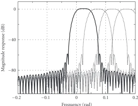
Figure8: Magnitude responses of the first 4 of the 64-band SBR complex-exponential modulated analysis filter bank. The magni-tude fork=0 is highlighted.
subband signals)Sk[q]:1
Sk[q]=s∗hk
[Kq]. (34)
The magnitude responses of the first 4 frequency bands (k = 0,. . ., 3) of the QMF analysis bank are illustrated in
Figure 8.
The down-sampled subband signals Sk[q] of the low-est QMF subbands are subsequently fed through a second complex-modulated filter bank (sub-filter bank) to further enhance the frequency resolution; the remaining subband signals are delayed to compensate for the delay which is in-troduced by the sub-filter bank. The output of the hybrid (i.e., combined) filter bank is denoted bySk,m[q], withkthe subband index of the initial QMF bank, andmthe filter in-dex of the sub-filter bank. To allow easy identification of the two filter banks and their outputs, the index k of the first filter bank will be denoted “subband index,” and the index mof the subfilter bank is denoted “sub-subband index.” The sub-filter bank has a filter order ofNs=12, and an impulse responseGk,m[q] given by
Gk,m[q]=gk[q] exp j 2π Mk
m+1
2
q−Ns 2
!
, (35)
withgk[q] the prototype window associated with QMF band k,qthe sample index, andMkthe number of sub-subbands in QMF subbandk (m = 0,. . .,Mk−1).Table 2 gives the number of sub-subbandsMkas a function of the QMF band k, for both the 34 and 20 analysis-band configurations. As an example, the magnitude response of the 4-band sub-filter
Table2: Specification ofMkfor the first 5 QMF subbands.
QMF subband (k) Mk(B=34) Mk(B=20)
0 12 8
1 8 4
2 4 4
3 4 1
4 4 1
bank (Mk=4) is given inFigure 9. Obviously, due to the lim-ited prototype length (Ns =12), the stop-band attenuation is only in the order of 20 dB.
As a result of this hybrid QMF filter-bank structure, 91 (for B = 34) or 77 (B = 20) down-sampled filter out-puts Sk,m[q] and their filtered (decorrelated) counterparts Sk,m,d[q] are available for further processing. The decorrela-tion filter can be implemented in various ways. An elegant method comprises a reverberator [24]; a low-complexity al-ternative consists of a (frequency-dependent) delay Tk of which the delay time depends on the QMF subband indexk. The next stage of the QMF-based spatial synthesis stage performs a mixing and phase-adjustment process. For each sub-subband signal pairSk,m[q],Sk,m,d[q], an output signal pairYk,m,1[q],Yk,m,2[q] is generated by
Yk,m,1[q] Yk,m,2[q]
=Rk,m
Sk,m[q] Sk,m,d[q]
. (36)
The mixing matrixRk,m is determined as follows. Each quartet of the parameters IID, IPD, OPD, and IC for a sin-gle parameter subbandbrepresents a certain frequency range and a certain moment in time. The frequency range depends on the specification of the encoder analysis frequency bands (i.e., the grouping of FFT bins), while the position in time depends on the encoder time-domain segmentation. If the encoder is designed properly, the time/frequency localization of each parameter quartet coincides with a certain sample in-dex in a sub-subband or set of sub-subbands in the QMF domain. For that particular QMF sample index, the mix-ing matrices are exactly the same as their FFT-based coun-terparts (as specified by (25)–(32)). For QMF sample in-dices in between, the mixing matrices are interpolated lin-early (i.e., its real and imaginary parts are interpolated indi-vidually).
The mixing process is followed by a pair of hybrid QMF synthesis filter banks (one for each output channel), which also consist of two stages. The first stage comprises summa-tion of the sub-subbandsmwhich stem from the same sub-bandk:
Yk,1[q]= Mk−1
m=0
Yk,m,1[q],
Yk,2[q]= Mk−1
m=0
Yk,m,2[q].
(37)
3 2 1 0
−1
−2
−3
Frequency (rad)
−30
−20
−10 0
M
ag
n
itude
response
(dB)
Figure9: Magnitude response of the 4-band sub-filter bank. The response form=0 is highlighted.
Finally, upsampling and convolution with synthesis fil-ters (which are similar to the QMF analysis filfil-ters as specified by (33)) results in the final stereo output signal.
The fact that the same filter-bank structure is used for both PS and SBR enables an easy and low-cost integration of SBR and parametric stereo in a single decoder structure (cf. [23,24,91,92]). This combination is known as enhanced aacPlus and is under consideration for standardization in MPEG-4 as the HE-AAC/PS profile [93]. The structure of the decoder is shown inFigure 10. The incoming bit stream is demultiplexed into a band-limited AAC bit stream, SBR parameters, and parametric-stereo parameters. The AAC bit stream is decoded by an AAC decoder and fed into a 32-band QMF analysis bank. The output of this filter bank is processed by the SBR stage and by the sub-filter bank as de-scribed inSection 7. The resulting full-bandwidth mono sig-nal is converted to stereo by the PS stage, which performs decorrelation and mixing. Finally, two hybrid QMF synthe-sis banks result in the final output signals. More details on enhanced aacPlus can be found in [23,92].
8. PERCEPTUAL EVALUATION
Bit stream Demux
AAC decoder
SBR parameters PS parameters
32 QMF analysis
Sub-filter bank
SBR
PS
Hybrid QMF synthesis
Hybrid QMF synthesis
Output 1
Output 2
Figure10: Structure of enhanced aacPlus.
only. To exclude quality limitations induced by other cod-ing processes besides parametric stereo, this experiment was performed without a mono coder. The second listening test was performed to derive the actual coding gain of parametric stereo in a complete coder. For this purpose, a comparison was made between a state-of-the-art stereo coder (i.e., aac-Plus) and the same coder extended with parametric stereo (e.g., enhanced aacPlus) as described inSection 7.
8.1. Listening test I
Nine listeners participated in this experiment. All listeners had experience in evaluating audio codecs and were specif-ically instructed to evaluate both the spatial audio qual-ity as well as other noticeable artifacts. In a double-blind MUSHRA test [94], the listeners had to rate the perceived quality of several processed items against the original (i.e., unprocessed) excerpts on a 100-point scale with 5 anchors. All excerpts were presented over Stax Lambda Pro head-phones. The processed items included
(1) encoding and decoding using a state-of-the-art MPEG-1 layer 3 (MP3) coder at a bit rate of 128 kbps stereo and using its highest possible quality settings; (2) encoding and decoding using the FFT-based
par-ametric-stereo coder as described above without mono coder (i.e., assuming transparent mono coding) oper-ating at 8 kbps;
(3) encoding and decoding using the FFT-based par-ametric-stereo coder without mono coder operating at a bit rate of 5 kbps (using 20 analysis frequency bands instead of 34);
(4) the original as hidden reference.
The 13 test excerpts are listed inTable 3. All items are stereo, 16-bit resolution per sample, at a sampling frequency of 44.1 kHz.
The subjects could listen to each excerpt as often as they liked and could switch in real time between the four versions of each item. The 13 selected items showed to be the most critical items from an 80-item test set for either parametric stereo or MP3 during development and in-between evalua-tions of the algorithms described in this paper. The items had a duration of about 10 seconds and contained a large variety of audio classes. The average scores of all subjects are shown
inFigure 11. The top panel shows mean MUSHRA scores for
8 kbps parametric stereo (black bars) and MP3 at 128 kbps (white bars) as a function of the test item. The rightmost bars indicate the mean across all test excerpts. Most excerpts
show very similar scores, except for excerpts 4, 8, 10, and 13. Excerpts 4 (“Harpsichord”) and 8 (“Plucked string”) show a significantly higher quality for parametric stereo. These items contain many tonal components, a property that is typically problematic for waveform coders due to the large audibility of quantization noise for such material. On the other hand, excerpts 10 (“Man in the long black coat”) and 13 (“Two voices”) have higher scores for MP3. Item 13 exhibits an (un-naturally) large amount of channel separation, which is par-tially lost after parametric-stereo decoding. On average, both coders have equal scores.
The middle panel shows results for the parametric-stereo coder working at 5 kbps (black bars) and 8 kbps (white bars). In most cases, the 8 kbps coder has a higher quality than the 5 kbps coder, except for excerpts 5 (“Castanets”) and 7 (“Glockenspiel”). On average, the quality of the 5 kbps coder is only marginally lower than for 8 kbps, which demonstrates the shallow bit-rate/quality slope for the parametric-stereo coder.
The bottom panel shows 128 kbps MP3 (white bars) against the hidden reference (black bars). As expected, the hidden reference scores are close to 100. For fragments 7 (“Glockenspiel”) and 10 (“Man in the long black coat”), the hidden reference scores lower than MP3 at 128 kbps, which indicates transparent coding.
Table3: Description of test material.
Item index Name Origin/artist
1 Starship Trooper Yes
2 Day tripper The Beatles
3 Eye in the sky Alan Parsons
4 Harpsichord MPEG si01
5 Castanets MPEG si02
6 Pitch pipe MPEG si03
7 Glockenspiel MPEG sm02
8 Plucked string MPEG sm03
9 Yours is no disgrace Yes
10 Man in the long black coat Bob Dylan
11 Vogue Madonna
12 Applause SQAM disk
13 Two voices Left=MPEG es03=English female
Right=MPEG es02=German male
Mean 13 12 11 10 9 8 7 6 5 4 3 2 1
Test fragment index 0
50 100
MUSHRA
sc
or
e
Mean 13 12 11 10 9 8 7 6 5 4 3 2 1
Test fragment index 0
50 100
MUSHRA
sc
or
e
Mean 13 12 11 10 9 8 7 6 5 4 3 2 1
Test fragment index 0
50 100
MUSHRA
sc
or
e
Figure 11: MUSHRA scores averaged across listeners as a func-tion of test item and various coder configurafunc-tions (see text). The upper panel shows the results for 8 kbps parametric stereo (black bars) against stereo MP3 at 128 kbps (white bars). The middle panel shows the results for 5 kbps parametric stereo (black bars) versus 8 kbps parametric stereo (white bars). The lower panel shows the hidden reference (black bars) versus MP3 at 128 kbps (white bars).
8.2. Listening test II
This test also employed MUSHRA [94] methodology and in-cluded 10 items which were selected for the MPEG-4 HE-AAC stereo verification test [95]. The following versions of each item were included in the test:
(1) the original as hidden reference;
(2) a first lowpass filtered anchor (3.5 kHz bandwidth); (3) a second lowpass filtered anchor (7 kHz bandwidth); (4) aacPlus (HE-AAC) encoded at a bitrate of 24 kbps; (5) aacPlus (HE-AAC) encoded at a bit rate of 32 kbps; (6) enhanced aacPlus (HE-AAC/PS) encoded at a
to-tal bit rate of 24 kbps. Twenty analysis bands were used, and no IPD or OPD parameters were transmit-ted. The average parameter update rate amounted to 46 milliseconds. For each frame, the required number of bits for the stereo parameters was calculated. The remaining number of bits was available for the mono coder (HE-AAC).
Two different test sites participated in the test, with 8 and 10 experienced subjects per site, respectively. All excerpts were presented over headphones. The results per site, aver-aged across excerpts, are given inFigure 12.
At both test sites, it was found that aacPlus with para-metric stereo (enhanced aacPlus) at 24 kbps achieves a re-spectable average subjective quality of around 70 on a MUSHRA scale. Moreover, at 24 kbps, the subjective quality of enhanced aacPlus is equal to aacPlus at 32 kbps and signif-icantly better than aacPlus at 24 kbps. These results indicate a coding gain for enhanced aacPlus of 25% over stereo aacPlus.
9. CONCLUSIONS