Matplotlib for Python Developers.pdf

(1)

Matplotlib for Python

Developers

Build remarkable publication quality plots the easy way

(2)

All rights reserved. No part of this book may be reproduced, stored in a retrieval system, or transmitted in any form or by any means, without the prior written permission of the publisher, except in the case of brief quotations embedded in critical articles or reviews.

Every effort has been made in the preparation of this book to ensure the accuracy of the information presented. However, the information contained in this book is sold without warranty, either express or implied. Neither the author, Packt Publishing, nor its dealers or distributors will be held liable for any damages caused or alleged to be caused directly or indirectly by this book.

Packt Publishing has endeavored to provide trademark information about all the companies and products mentioned in this book by the appropriate use of capitals. However, Packt Publishing cannot guarantee the accuracy of this information.

First published: November 2009

Production Reference: 2221009

Published by Packt Publishing Ltd. 32 Lincoln Road

Olton

Birmingham, B27 6PA, UK. ISBN 978-1-847197-90-0 www.packtpub.com

(3)

Credits

Author Sandro Tosi

Reviewers

Michael Droettboom Reinier Heeres

Acquisition Editor Usha Iyer

Development Editor Rakesh Shejwal

Technical Editor Namita Sahni

Copy Editor Leonard D'Silva

Indexers Monica Ajmera Hemangini Bari

Editorial Team Leader Akshara Aware

Project Team Leader Priya Mukherji

Project Coordinator Zainab Bagasrawala

Proofreader Lesley Harrison

Graphics Nilesh Mohite

Production Coordinator Adline Swetha Jesuthas

Cover Work

(4)

About the Author

Sandro Tosi

was born in Firenze (Italy) in the early 80s, and graduated with a B.Sc. in Computer Science from the University of Firenze.

His personal passions for Linux, Python (and programming), and computer

technology are luckily a part of his daily job, where he has gained a lot of experience in systems and applications management, database administration, as well as project management and development.

After having worked for five years as an EAI and an Application architect in an energy multinational, he's now working as a system administrator for an important European Internet company.

(5)

About the Reviewers

Michael Droettboom

holds a Master's Degree in Computer Music Research from The Johns Hopkins University. His research in optical music recognition lead to the development of the Gamera document image analysis framework, which has been used to recognize features in documents as diverse as medieval manuscript, Navajo texts, historical Scottish census data, and early American sheet music. His focus on computer graphics has lead to specializations in consumer electronics, computer-assisted engineering, and most recently, the science software for the Space Telescope Science Institute. He is currently one of the most active developers on the Matplotlib project.

I wish to thank my son, Kai, for asking all the hard questions.

Reinier

Heeres

has an MSc degree in Applied Physics from the Delft University of Technology, The Netherlands. He is currently pursuing a PhD there in the Quantum Transport group of the nanoscience department.

He has previously worked on Sugar, the child-friendly user interface mainly in use by One Laptop Per Child's $100 laptop. For this project, he designed the Calculator application.

(6)

(7)

Chapter 2: Getting Started with Matplotlib

21

First plots with Matplotlib 21

Multiline plots 25

A brief introduction to NumPy arrays 27

Grid, axes, and labels 28

Adding a grid 28

Handling axes 29

Adding labels 31

(8)

A complete example 35

Saving plots to a file 36

Interactive navigation toolbar 38

IPython support 40

Controlling the interactive mode 42

Suppressing functions output 43

Configuring Matplotlib 43

Configuration files 44

Configuring through the Python code 45

Selecting backend from code 46

Summary 47

Chapter 3: Decorate Graphs with Plot Styles and Types

49

Markers and line styles 49

Control colors 50

Specifying styles in multiline plots 52

Control line styles 52

Control marker styles 53

Finer control with keyword arguments 56

Handling X and Y ticks 58

Plot types 59

Histogram charts 59

Error bar charts 61

Bar charts 63

Pie charts 67

Scatter plots 69

Polar charts 71

Navigation Toolbar with polar plots 73

Control radial and angular grids 73

Text inside figure, annotations, and arrows 74

Text inside figure 74

Annotations 75

Arrows 77

Summary 79

Chapter 4: Advanced Matplotlib

81

Object-oriented versus MATLAB styles 81

A brief introduction to Matplotlib objects 85

Our first (simple) example of OO Matplotlib 85

Subplots 86

Multiple figures 88

(9)

Logarithmic axes 91

Share axes 92

Plotting dates 94

Date formatting 95

Axes formatting with axes tick locators and formatters 96

Custom formatters and locators 99

Text properties, fonts, and LaTeX 99

Fonts 101

Using LaTeX formatting 102

Mathtext 103

External TeX renderer 104

Contour plots and image plotting 106

Contour plots 106

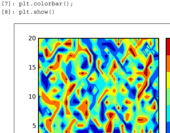
Image plotting 109

Summary 111

Chapter 5: Embedding Matplotlib in GTK+

113

A brief introduction to GTK+ 113

Introduction to GTK+ signal system 115

Embedding a Matplotlib figure in a GTK+ window 116

Including a navigation toolbar 119

Real-time plots update 123

Embedding Matplotlib in a Glade application 132

Designing the GUI using Glade 132

Code to use Glade GUI 135

Summary 144

Chapter 6: Embedding Matplotlib in Qt 4

145

Brief introduction to Qt 4 and PyQt4 145

Embedding a Matplotlib figure in a Qt window 147

Including a navigation toolbar 151

Real-time update of a Matplotlib graph 156

Embedding Matplotlib in a GUI made with Qt Designer 165

Designing the GUI using Qt Designer 165

Code to use the Qt Designer GUI 168

Introduction to signals and slots 171

Returning to the example 172

Summary 179

Chapter 7: Embedding Matplotlib in wxWidgets

181

(10)

Real-time plots update 192 Embedding Matplotlib in a GUI made with wxGlade 203

Summary 213

Chapter 8: Matplotlib for the Web

215

Matplotlib and CGI 216

What is CGI 216

Configuring Apache for CGI execution 216

Simple CGI example 218

Matplotlib in a CGI script 219

Passing parameters to a CGI script 220

Matplotlib and mod_python 223

What is mod_python 223

Apache configuration for mod_python 224

Matplotlib in a mod_python example 226

Matplotlib and mod_python's Python Server Pages 228

Web Frameworks and MVC 231

Matplotlib and Django 232

What is Django 232

Matplotlib in a Django application 233

Matplotlib and Pylons 237

What is Pylons 237

Matplotlib in a Pylons application 238

Summary 242

Chapter 9: Matplotlib in the Real World

243

Plotting data from a database 244

Plotting data from the Web 247

Plotting data by parsing an Apache log file 250

Plotting data from a CSV file 256

Plotting extrapolated data using curve fitting 261

Tools using Matplotlib 267

NetworkX 267

Mpmath 269

Plotting geographical data 271

First example 272

Using satellite background 274

Plot data over a map 275

Plotting shapefiles with Basemap 277

Summary 279

(11)

Preface

This book is about Matplotlib, a Python package for 2D plotting that generates production quality graphs. Its variety of output formats, several chart types, and capability to run either interactively (from Python or IPython consoles) and non-interactively (useful, for example, when included into web applications), makes Matplotlib suitable for use in many different situations.

Matplotlib is a big package with several dependencies and having them all installed and running properly is the first step that needs to be taken. We provide some ways to have a system ready to explore Matplotlib. Then we start describing the basic functions required for plotting lines, exploring any useful or advanced commands for our plots until we come to the core of Matplotlib: the object-oriented interface. This is the root for the next big section of the book—embedding Matplotlib into GUI libraries applications. We cannot limit it only to desktop programs, so we show several methods to include Matplotlib into web sites using low level techniques for two well known web frameworks—Pylons and Django. Last but not the least, we present a number of real world examples of Matplotlib applications.

The core concept of the book is to present how to embed Matplotlib into Python applications, developed using the main GUI libraries: GTK+, Qt 4, and wxWidgets. However, we are by no means limiting ourselves to that. The step-by-step

(12)

What this book covers

Chapter 1—Introduction to Matplotlib introduces what Matplotlib is, describing its output formats and the interactions with graphical environments. Several ways to install Matplotlib are presented, along with its dependencies needed to have a correctly configured environment to get along with the book.

Chapter 2—Getting started with Matplotlib covers the first examples of Matplotlib usage. While still being basic, the examples show important aspects of Matplotlib like how to plot lines, legends, axes labels, axes grids, and how to save the finished plot. It also shows how to configure Matplotlib using its configuration files or directly into the code, and how to work profitable with IPython.

Chapter 3—Decorate Graphs with Plot Styles and Types discusses the additional plotting capabilities of Matplotlib: lines and points styles and ticks customizations. Several types of plots are discussed and covered: histograms, bars, pie charts, scatter plots, and more, along with the polar representation. It is also explained how to include textual information inside the plot.

Chapter 4—Advanced Matplotlib examines some advanced (or not so common) topics like the object-oriented interface, how to include more subplots in a single plot or how to generate more figures, how to set one axis (or both) to logarithmic scale, and how to share one axis between two graphs in one plot. A consistent section is dedicated to plotting date information and all that comes with that. This chapter also shows the text properties that can be tuned in Matplotlib and how to use the LaTeX typesetting language. It also presents a section about contour plot and image plotting.

Chapter 5—Embedding Matplotlib in GTK+ guides us through the steps to embed Matplotlib inside a GTK+ program. Starting from embedding just the Figure and the Navigation toolbar, it will present how to use Glade to design a GUI and then embed Matplotlib into it. It also describes how to dynamically update a Matplotlib plot using the GTK+ capabilities.

Chapter 6—Embedding Matplotlib in Qt 4 explores how to include a Matplotlib figure into a Qt 4 GUI. It includes an example that uses Qt Designer to develop a GUI and how to use Matplotlib into it. What Qt 4 library provides for a real-time update of a Matplotlib plot is described here too.

(13)

Chapter 8—Matplotlib for the Web describes how to expose plots generated with Matplotlib on the Web. The first examples start from the lower ground, using CGI and the Apache mod_python module, technologies recommended only for limited or simple tasks. For a full web experience, two web frameworks are introduced, Pylons and Django, and a complete guide for the inclusion of Matplotlib with these frameworks is given.

Chapter 9—Matplotlib in the Real World takes Matplotlib and brings it into the real world examples field, guiding through several situations that might occur in the real life. The source code to plot the data extracted from a database, a web page, a parsed log file, and from a comma-separated file are described in full detail here. A couple of third-party tools using Matplotlib, NetworkX, and Mpmath, are described presenting some examples of their usage. A considerable section is dedicated to Basemap, a Matplotlib toolkit to draw geographical data.

What you need for this book

In order to be able to have the best experience with this book, you have to start with an already working Python environment, and then follow the advice in Chapter 1 on how to install Matplotlib and its most important dependencies. Some examples require additional tools, libraries, or modules to be installed: consult the distribution or project documentation for installation details.

Python, Matplotlib, and all other tools are cross-platform, so the book examples can be executed on Linux, Windows, or Mac OS X.

The book and the example code was developed using Python 2.5 and Matplotlib 0.98.5.3, but due to recent developments, Python 2.6 (Python 3.x is still not well supported by NumPy, Matplotlib, and several other modules) and Matplotlib 0.99.x can be used as well.

Who this book is for

This book is essentially for Python developers who have a good knowledge of Python; no knowledge of Matplotlib is required. You will be creating 2D plots using Matplotlib in no time at all.

Conventions

(14)

Code words in text are shown as follows: "This is used for enhanced handling of the datetime Python objects."

A block of code is set as follows:

In [1]: import matplotlib.pyplot as plt In [2]: import numpy as np

In [3]: y = np.arange(1, 3) In [4]: plt.plot(y, 'y'); In [5]: plt.plot(y+1, 'm'); In [6]: plt.plot(y+2, 'c'); In [7]: plt.show()

When we wish to draw your attention to a particular part of a code block, the relevant lines or items are set in bold:

c[0]*x**deg + c[1]*x**(deg – 1) + ... + c[deg]

Any command-line input or output is written as follows:

$ easy_install matplotlib-<version>-py<py version>-win32.egg

New terms and important words are shown in bold. Words that you see on the screen, in menus or dialog boxes for example, appear in the text like this: "There are several aspects we might want to tune in a widget, and this can be done using the Properties window."

Warnings or important notes appear in a box like this.

Tips and tricks appear like this.

Reader feedback

Feedback from our readers is always welcome. Let us know what you think about this book—what you liked or may have disliked. Reader feedback is important for us to develop titles that you really get the most out of.

(15)

If there is a book that you need and would like to see us publish, please send us a note in the SUGGEST A TITLE form on www.packtpub.com or email

[email protected].

If there is a topic that you have expertise in and you are interested in either writing or contributing to a book on, see our author guide on www.packtpub.com/authors.

Customer support

Now that you are the proud owner of a Packt book, we have a number of things to help you to get the most from your purchase.

Downloading the example code for the book

Visit http://www.packtpub.com/files/code/7900_Code.zip to directly download the example code.

The downloadable files contain instructions on how to use them.

Errata

Although we have taken every care to ensure the accuracy of our content, mistakes do happen. If you find a mistake in one of our books—maybe a mistake in the text or the code—we would be grateful if you would report this to us. By doing so, you can save other readers from frustration, and help us to improve subsequent versions of this book. If you find any errata, please report them by visiting http://www.packtpub. com/support, selecting your book, clicking on the let us know link, and entering the details of your errata. Once your errata are verified, your submission will be accepted and the errata added to any list of existing errata. Any existing errata can be viewed by selecting your title from http://www.packtpub.com/support.

Piracy

Piracy of copyright material on the Internet is an ongoing problem across all media. At Packt, we take the protection of our copyright and licenses very seriously. If you come across any illegal copies of our works, in any form, on the Internet, please provide us with the location address or web site name immediately so that we can pursue a remedy.

(16)

Questions

(17)

Introduction to Matplotlib

A picture is worth a thousand words.

We all know that images are a powerful form of communication. We often use them to understand a situation better or to condense pieces of information into a graphical representation.

Just to give a couple of examples on how helpful they can be, let's consider the scientific and performance analysis fields. In order to clearly identify the bottlenecks, it is very important to be able to visualize data when analyzing performance

information. Similarly, taking a quick glance at a graph drawn for a scientific experiment can give a scientist a better understanding of the results, something which is harder to achieve by looking only at the raw data.

Python is an interpreted language with a strong core functions basis and a powerful modular aspect which allows us to expand the language with external modules that offer new functionalities.

Modules reflect the Unix philosophy:

Do one thing, do it well.

(18)

Matplotlib is a Python package for 2D plotting that generates production-quality graphs. It supports interactive and non-interactive plotting, and can save images in several output formats (PNG, PS, and others). It can use multiple window toolkits (GTK+, wxWidgets, Qt, and so on) and it provides a wide variety of plot types (lines, bars, pie charts, histograms, and many more). In addition to this, it is highly customizable, flexible, and easy to use.

The dual nature of Matplotlib allows it to be used in both interactive and non-interactive scripts. It can be used in scripts without a graphical display, embedded in graphical applications, or on web pages. It can also be used interactively with the Python interpreter or IPython.

In this chapter, we will introduce Matplotlib, learn what it is, and what it can do. Later on, we will see what tools and Python modules are needed to have the best experience with Matplotlib and how to get them installed on our system, be it Linux, Windows, or Mac OS X.

The topics we are going to cover are: • Introduction to Matplotlib • Output formats and backends • Dependencies

• How to install Matplotlib

Merits of Matplotlib

The idea behind Matplotlib can be summed up in the following motto as quoted by John Hunter, the creator and project leader of Matplotlib:

Matplotlib tries to make easy things easy and hard things possible.

We can generate high quality, publication-ready graphs with minimal effort (sometimes we can achieve this with just one line of code or so), and for elaborate graphs, we have at hand a powerful library to support our needs.

Matplotlib was born in the scientific area of computing, where gnuplot and MATLAB were (and still are) used a lot.

(19)

We have to think of plotting not just as the final step in working with our data, but as an important way of getting visual feedback during the process. Here, the interactive capabilities of Matplotlib will come and rescue us.

Matplotlib was modeled on MATLAB, because graphing was something that MATLAB did very well. The high degree of compatibility between them made many people move from MATLAB to Matplotlib, as they felt like home while working with Matplotlib.

But what are the points that built the success of Matplotlib? Let's look at some of them: • It usesPython: Python is a very interesting language for scientific purposes

(it's interpreted, high-level, easy to learn, easily extensible, and has a powerful standard library) and is now used by major institutions such as NASA, JPL, Google, DreamWorks, Disney, and many more.

• It's open source, so no license to pay: This makes it very appealing for professors and students, who often have a low budget.

• It'sarealprogramminglanguage: The MATLAB language (while being Turing-complete) lacks many of the features of a general-purpose language

like Python.

• It'smuchmore complete: Python has a lot of external modules that will help us perform all the functions we need to. So it's the perfect tool to acquire data, elaborate the data, and then plot the data.

• It'sverycustomizableandextensible: Matplotlib can fit every use case because it has a lot of graph types, features, and configuration options. • It'sintegratedwithLaTeXmarkup: This is really useful when writing

scientific papers.

• It'scross-platformandportable: Matplotlib can run on Linux, Windows, Mac OS X, and Sun Solaris (and Python can run on almost every

architecture available).

(20)

Matplotlib web sites and online

documentation

The official Matplotlib presence on the Web is made up of two web sites: • The SourceForge project page at http://sourceforge.net/projects/

matplotlib/

• The main web site at http://matplotlib.sourceforge.net/

The SourceForge page contains, in particular, information about the development of Matplotlib, such as the released source code tarballs and binary packages, the SVN repository location, the bug tracking system, and so on. SourceForge also hosts some mailing lists for Matplotlib which are used for developers' discussions and users support.

On the main web site, we can find several important pieces of information about the Matplotlib package itself. For example:

• It contains a very attractive gallery with a huge number of examples of what Matplotlib can do

• The official documentation of Matplotlib is also present on this web site The official documentation for Matplotlib is extensive. It covers in detail, all the submodules and the methods exposed by them, including all of their arguments. There are too many function arguments to cover in this book, so we are presenting only the most common ones here. In case of any doubts or questions, the official documentation is a good place to start your research or to look for an answer. We encourage you to take a look at the gallery—it's inspiring!

Output formats and backends

The aim of Matplotlib is to generate graphs. So, we need a way to actually view

(21)

Output formats

Given its scientific roots (that means several different needs), Matplotlib has a lot of output formats available, which can be used for articles/books and other print publications, for web pages, or for any other reason we can think of. Let's first differentiate the output formats into two distinct categories:

• Raster images: These are the classic images we can find on the Web or used for pictures. The most well known raster file formats are PNG, JPG, and BMP. They are widespread and well supported. The format of these images is like a matrix, with rows and columns, and at every matrix cell we have a pixel description (containing information such as colors). This format is said to be

resolution-dependent, because the size of the matrix (the number of rows and columns) is determined when the image is created. An important parameter for raster images is the DPI (dots-per-inch) value. Once the image dimensions are decided (length and width, in inches), the DPI value specifies the detail level of the image. Hence, higher the DPI value, higher is the quality of the image (because for the same inch we get more dots). Scaling operations such as zooming or resizing can result in a loss of quality, because the image contains only a limited amount of information.

• Vector images: As opposed to raster images, vector images contain a description of the image in the form of mathematical equations and geometrical primitives (for example, points, lines, curves, polygons, or shapes). We can think of this format as a series of directives to plot the image: "Draw a point here, draw another point there, draw a line between those two points" and so on. Given this descriptive format, these images are said to be

resolution-independent, because it's the image interpreter that replots the image at the requested resolution using the instructions in it. Typical examples of vector image usage are typesetting and CAD (architectural or mechanical parts drawings).

Of course, Matplotlib supports both the categories, particularly with the following output formats:

Format Type Description

EPS Vector Encapsulated PostScript.

JPG Raster Graphic format with lossy compression method for photographic output.

PDF Vector Portable Document Format (PDF).

(22)

PS or EPS formats are particularly useful for plots inclusion in LaTeX documents, the main scientific articles format since decades.

Backends

In the previous section, we saw the file output formats—they are also called hardcopybackendsas they create something (a file on disk).

A backend that displays the image on screen is called a userinterfacebackend. The backend is that part of Matplotlib that works behind the scenes and allows the software to target several different output formats and GUI libraries (for screen visualization).

In order to be even more flexible, Matplotlib introduces the following two layers structured (only for GUI output):

• The renderer: This actually does the drawing • The canvas: This is the destination of the figure

The standard renderer is the Anti-GrainGeometry (AGG) library, a high performance rendering engine which is able to create images of publication level quality, with anti-aliasing, and subpixel accuracy. AGG is responsible for the beautiful appearance of Matplotlib graphs.

The canvas is provided with the GUI libraries, and any of them can use the AGG rendering, along with the support for other rendering engines (for example, GTK+). Let's have a look at the user interface toolkits and their available renderers:

Backend Description

GTKAgg GTK+ (The GIMP ToolKit GUI library) canvas with AGG rendering.

GTK GTK+ canvas with GDK rendering. GDK rendering is rather primitive, and doesn't include anti-aliasing for the smoothing of lines.

GTKCairo GTK+ canvas with Cairo rendering.

WxAgg wxWidgets (cross-platform GUI and tools library for GTK+, Windows,

and Mac OS X. It uses native widgets for each operating system, so applications will have the look and feel that users expect on that operating system) canvas with AGG rendering.

WX wxWidgets canvas with native wxWidgets rendering.

(23)

Backend Description

QtAgg Qt (cross-platform application framework for desktop and embedded development) canvas with AGG rendering (for Qt version 3 and earlier).

Qt4Agg Qt4 canvas with AGG rendering.

FLTKAgg FLTK (cross-platform C++ GUI toolkit for UNIX/Linux (X11), Microsoft

Windows, and Mac OS X) canvas with Agg rendering.

Here is the list of renderers for file output:

Renderer File type

AGG .png

PS .eps or .ps

PDF .pdf

SVG .svg

Cairo .png, .ps, .pdf, .svg

GDK .png, .jpg

The renderers mentioned in the previous table can be used directly in Matplotlib, when we want only to save the resulting graph into a file (without any visualization of it), in any of the formats supported.

We have to pay attention when choosing which backend to use. For example, if we don't have a graphical environment available, then we have to use the AGG backend (or any other file). If we have installed only the GTK+ Python bindings, then we can't use the WX backend.

About dependencies

As mentioned earlier, Matplotlib has its origin in scientific fields, so it is commonly used to plot huge datasets. Python's native support for long lists becomes impractical for such sizes, so Matplotlib needs better support for arrays.

NumPy, the de facto standard Python module for numerical elaborations, provides support for high performance operations even with big mathematical data types such as arrays or matrices—along with many other mathematical functions that can be useful to Matplotlib users.

(24)

Once we have chosen the set of user interfaces (UIs) we prefer, then we need to install the Python bindings for them. Here is a summarizing list:

User Interface

(UI) Binding Version Description

FLTK pyFLTK 1.0 or

higher pyFLTK provides Python wrappers for the FLTK widgets library for use with FLTKAgg backend.

GTK+ PyGTK 2.2 or

higher PyGTK provides Python wrappers for the GTK+ widgets library to use it with the GTK or GTKAgg

backend.

It is recommended to use a version higher than 2.12, for a correct memory management. Qt PyQt or

PyQt4 3.1 or higher and for Qt4, 4.0 or higher

PyQt or PyQt4 provides Python wrappers for the Qt toolkit and is required by the Matplotlib QtAgg

and Qt4Agg backends. The library is widely used

on Linux and Windows.

Tk PyTK 8.3 or

higher Python wrapper for Tcl or Tk widgets library is used in TkAgg backend.

Wx wxPython 2.6 or higher, or 2.8 or higher

wxPython provides Python wrappers for the

wxWidgets library for use with the WX and WXAgg

backends. It is widely used on Linux, Mac OS X,

and Windows.

Another important tool, in particular for interactive usage, is IPython. It's an interactive Python shell with a lot of useful features, such as history, commands repeating, and others. It already has a Matplotlibmode in it. We'll be using IPython in this book, so it is recommended to install it.

Some of the tools that are needed by Matplotlib are already shipped with it (in the source code as well as in the binary distributions). Here is the list of those tools:

• AGG (version 2.4): This is the Anti-Grain Geometry rendering engine. The local copy of the library is linked with the Matplotlib code in a static way. So, there's no need to install it (as a shared library).

• pytz (version 2007g or higher): This is used for handling the time zone for datetime Python objects. It will be installed if it's not already present in the system. It can be overridden using setup.cfg.

(25)

Build dependencies

The following tools are needed if we're going to install Matplotlib from the source: • Python: Currently, only Python 2.x is supported (no Python 3 yet)

• NumPy: Version 1.1 or higher

• libpng: Version 1.1 or higher is needed to load or save PNG images (Windows users can skip this requirement)

• FreeType: Version 1.4 or higher is needed for reading TrueType font files (Windows users can skip this requirement)

libpng and FreeType for Windows users are already packaged in the Matplotlib Windows installer.

Installing Matplotlib

There are several ways to install Matplotlib on our system: • Using packages from a Linux distribution

• Using binary installers (for Windows and Mac OS X only)

• Using packaged Python distributions that contain Matplotlib in the toolbox proposed

• From the source code

We will look at each option in detail. We assume that Python, NumPy, and the optional build and runtime dependencies are already installed in the system (in order to install them, refer to their installation guides).

Installing Matplotlib on Linux

(26)

In the following table, we will present some of the common Linux distributions package names for Matplotlib and the tools we can use to install the package:

Distribution Package name Installer tool

Debian or Ubuntu (and all other Debian derivatives)

python-matplotlib Synaptic (graphical)

apt-get or aptitude (command line)

Fedora python-matplotlib PackageKit (graphical) yum or rpm (command line) openSUSE python-matplotlib YaST (graphical)

zipper or rpm (command line)

Installing Matplotlib on Windows

Before we can install Matplotlib, we have to satisfy its main dependencies. So, we have to download:

• Installers for Python, which are available in the DOWNLOAD section of http://www.python.org/

• Installers for NumPy, which are available in the Download section of http://www.scipy.org/

Once we've got the above packages correctly installed, we can go to the main project page of Matplotlib on SourceForge at http://sourceforge.net/projects/

matplotlib/. In the Files section, we can find the relative versions of the binary packages for the Python that we have just installed (2.4, 2.5, or 2.6).

Installing Matplotlib on Mac OS X

The procedure to install Matplotlib correctly on Mac OS X is similar to that of Windows.

First of all, we need to download:

• Installers for Python, which are available in the DOWNLOAD section of http://www.python.org/ (the one already available in Mac OS X fives problem when using Matplotlib)

(27)

At this point, once they are correctly installed, we can download the binary installer from the download area of Matplotlib SourceForce page at

http://sourceforge.net/projects/matplotlib/ or we can retrieve the version available at http://pythonmac.org/.

Installing Matplotlib using packaged

Python distributions

There are some packaged distributions of Python that contain Matplotlib in them, along with many other tools, such as IPython, NumPy, SciPy, and so on. These distributions will set up all the necessary things we need so that we can use Matplotlib on our machine. Some of the distributions are as follows:

• EnthoughtPythonDistribution (EPD): This package is available for Windows, Mac OS X, and Red Hat. We can download it from

http://www.enthought.com/products/epd.php.

• Python(x,y): This package is available for Windows and Ubuntu at http://www.pythonxy.com/.

• Sage: This package is available for Linux at http://www.sagemath.org/. These are mainly scientific distributions that install a lot of tools we don't directly need or use, but they have the advantage of making it easy to get Python, NumPy, and Matplotlib installed and working on our system.

Installing Matplotlib from source code

There are two ways of obtaining the Matplotlib source code. They are:

• Downloading it from the source code tarballs available in the download area of Matplotlib SourceForge project page at http://sourceforge.net/ projects/matplotlib/.

• Retrieving it from the Subversion (SVN) repository. This is the

place where development takes place, so use it only if you know what you're doing.

(28)

If we are going to use the source code tarball, we will have to unpack it, go into the created source directory, and execute the following commands:

$ python setup.py build

$ sudo python setup.py install

These commands will build and then install Matplotlib. We will need administrative privileges to install it into the system directories (hence the sudo command in this Linux example).

Many aspects of the installation can be tuned using setup.cfg, a file shipped with the source code and used at build and install time. We can use it to customize the build process, such as changing the default backend, or choosing whether to install the optional libraries or not.

If we want to install Matplotlib from source on Windows, the Files section of Matplotlib SourceForge page contains handy egg files which we can download (choosing the Python version of interest) and then install using setuptools command. The following command will install Matplotlib on your machine:

$ easy_install matplotlib-<version>-py<py version>-win32.egg

Egg files are also available for Mac OS X, and we can use them in the same way as described above.

Testing our installation

To ensure we have correctly installed Matplotlib and its dependencies, a very simple test can be carried out in the following manner:

$ python

Python 2.5.4 (r254:67916, Feb 18 2009, 03:00:47) [GCC 4.3.3] on linux2

Type "help", "copyright", "credits" or "license" for more information. >>> import numpy

>>> print numpy.__version__ 1.2.1

>>> import matplotlib

>>> print matplotlib.__version__

0.98.5.3

(29)

Summary

In this chapter, we have covered the following areas: • What is Matplotlib and what are its main key points

• The several file output formats and graphical user interfaces (GUIs) that are supported

• The packages required by Matplotlib, and the ones needed for the GUI bindings

• Installing and testing Matplotlib on a Linux, Windows, or Mac OS X system, in multiple ways

(30)

(31)

Getting Started with

Matplotlib

In the previous chapter, we have given a brief introduction to Matplotlib. We now want to start using it for real—after all, that's what you are reading this book for. In this chapter, we will:

• Explore the basic plotting capabilities of Matplotlib for single or multiple lines

• Add information to the plots such as legends, axis labels, and titles • Save a plot to a file

• Describe the interaction with IPython

• Customize Matplotlib, both through configuration files and Python code Let's start looking at some graphs.

First plots with Matplotlib

One of the strong points of Matplotlib is how quickly we can start producing plots out of the box. Here is our first example:

$ ipython

In [1]: import matplotlib.pyplot as plt In [2]: plt.plot([1, 3, 2, 4])

(32)

This code snippet gives the output shown in the following screenshot:

As you can see, we are using IPython. This will be the case throughout the book, so we'll skip the command execution line (and the heading) as you can easily recognize IPython output.

Let's look at each line of the previous code in detail: In [1]: import matplotlib.pyplot as plt

This is the preferred format to import the main Matplotlib submodule for plotting, pyplot. It's the best practice and in order to avoid pollution of the global namespace, it's strongly encouraged to never import like:

from <module> import *

The same import style is used in the official documentation, so we want to be consistent with that.

(33)

This code line is the actual plotting command. We have specified only a list of values that represent the vertical coordinates of the points to be plotted. Matplotlib will use an implicit horizontal values list, from 0 (the first value) to N-1 (where N is the number of items in the list).

If you remember from high school, the vertical values represent the Y-axis while the horizontal values are the X-axis, and what we do is called "to plot Y against X".

In [3]: plt.show()

This command actually opens the window containing the plot image. Of course, we can also explicitly specify both the lists:

In [1]: import matplotlib.pyplot as plt In [2]: x = range(6)

In [3]: plt.plot(x, [xi**2 for xi in x])

Out[3]: [<matplotlib.lines.Line2D object at 0x2408d10>] In [4]: plt.show()

(34)

As we can see, the line shown in the previous screenshot has several edges, while we might want a smoother parabola. So, we can start introducing the interaction with NumPy with one of its most used functions, arange(), and highlighting the difference with range():

• range(i, j, k) is a Python built-in function that generates a sequence of integers from i to j with an increment of k (both, the initial value and the step are optional).

• arange(x, y, z) is a part of NumPy, and it generates a sequence of elements (with data type determined by parameter types) from x to y with a spacing z (with the same optional parameters as that of the previous function).

So we can use arange() to generate a finer range:

In [3]: x = np.arange(0.0, 6.0, 0.01) In [4]: plt.plot(x, [x**2 for x in x])

(35)

Multiline plots

It's fun to plot a line, but it's even more fun when we can plot more than one line on the same figure. This is really easy with Matplotlib as we can simply plot all the lines that we want before calling show(). Have a look at the following code and screenshot:

In [1]: import matplotlib.pyplot as plt In [2]: x = range(1, 5)

In [3]: plt.plot(x, [xi*1.5 for xi in x])

Out[3]: [<matplotlib.lines.Line2D object at 0x2076ed0>] In [4]: plt.plot(x, [xi*3.0 for xi in x])

Out[4]: [<matplotlib.lines.Line2D object at 0x1e544d0>] In [5]: plt.plot(x, [xi/3.0 for xi in x])

Out[5]: [<matplotlib.lines.Line2D object at 0x20864d0>] In [6]: plt.show()

(36)

plot() supports another syntax useful in this situation. We can plot multiline figures by passing the X and Y values list in a single plot() call:

In [1]: import matplotlib.pyplot as plt In [2]: x = range(1, 5)

In [3]: plt.plot(x, [xi*1.5 for xi in x], x, [xi*3.0 for xi in x], x, [xi/3.0 for xi in x])

Out[3]:

[<matplotlib.lines.Line2D object at 0x1d4bed0>, <matplotlib.lines.Line2D object at 0x1d56fd0>, <matplotlib.lines.Line2D object at 0x1d5d3d0>] In [4]: plt.show()

The preceding code simply rewrites the previous example with a different syntax. While list comprehensions are a very powerful tool, they can generate a little bit of confusion in these simple examples. So we'd like to show another feature of the arange() function of NumPy:

In [3]: x = np.arange(1, 5)

In [4]: plt.plot(x, x*1.5, x, x*3.0, x, x/3.0) Out[4]:

[<matplotlib.lines.Line2D object at 0x15d5d10>, <matplotlib.lines.Line2D object at 0x15ddf90>, <matplotlib.lines.Line2D object at 0x15e4390>] In [5]: plt.show()

Here, we take advantage of the NumPy array objects returned by arange(). The multiline plot is possible because, by default, the hold property is enabled (consider it as a declaration to preserve all the plotted lines on the current figure instead of replacing them at every plot() call). Try this simple example and see what happens:

In [1]: import matplotlib.pyplot as plt

In [2]: plt.interactive(True)# enable interactive mode, in case it was not

In [3]: plt.hold(False) # empty window will pop up In [4]: plt.plot([1, 2, 3])

Out[4]: [<matplotlib.lines.Line2D object at 0x19ea1d0>] In [5]: plt.plot([2, 4, 6])

Out[5]: [<matplotlib.lines.Line2D object at 0x19e8cd0>]

(37)

A brief introduction to NumPy arrays

In the previous section, we've mentioned NumPy array objects (in relation to arange()), but they deserve a proper introduction because we will be using them throughout this book.

Python lists are extremely flexible and really handy, but when dealing with a large number of elements or to support scientific computing, they show their limits. One of the fundamental aspects of NumPy is providing a powerful N-dimensional array object, ndarray, to represent a collection of items (all of the same type). Creating an array (an object of type ndarray) is simple:

In [1]: import numpy as np In [2]: x = np.array([1, 2, 3]) In [3]: x

Out[3]: array([1, 2, 3])

We can pass a list or a tuple to array() and in return, we have an array object. We can treat this array as if it was a list; we can slice it or select one of its elements using the standard Python syntax:

In [4]: x[1:]

Out[4]: array([2, 3]) In [5]: x[2]

Out[5]: 3

As we have already seen, we can operate on the whole array (this kind of operation is common in MATLAB):

In [6]: x*2

Out[6]: array([2, 4, 6])

This code snippet returns a new array with the elements of x multiplied by 2; if we were working with a list, we would have had to use a list comprehension:

In [7]: l = [1, 2, 3] In [8]: [2*li for li in l] Out[8]: [2, 4, 6]

We can work with more arrays and make them interact: In [9]: a = np.array([1, 2, 3])

(38)

We can also create multidimensional arrays:

In [12]: M = np.array([[1, 2, 3], [4, 5, 6]]) In [13]: M[1,2]

Out[13]: 6

Another important function—the one that we already met, is arange(): In [14]: range(6)

Out[14]: [0, 1, 2, 3, 4, 5] In [15]: np.arange(6)

Out[15]: array([0, 1, 2, 3, 4, 5])

It mimics the range() function from the core Python but it returns a NumPy array.

Grid, axes, and labels

Now we can learn about some features that we can add to plots, and some features to control them better.

Adding a grid

In the previous images, we saw that the background of the figure was completely blank. While it might be nice for some plots, there are situations where having a reference system would improve the comprehension of the plot—for example with multiline plots. We can add a grid to the plot by calling the grid() function; it takes one parameter, a Boolean value, to enable (if True) or disable (if False) the grid:

[<matplotlib.lines.Line2D object at 0x8fcc20c>, <matplotlib.lines.Line2D object at 0x8fcc50c>, <matplotlib.lines.Line2D object at 0x8fcc84c>] In [5]: plt.grid(True)

In [6]: plt.show()

(39)

Handling axes

You might have noticed that Matplotlib automatically sets the limits of the figure to precisely contain the plotted datasets. However, sometimes we want to set the axes limits ourself (defining the scale of the chart). Let's take the first multiline plot. Wouldn't it be better to have more spaces between lines and borders? We can achieve this with the following code:

[<matplotlib.lines.Line2D object at 0x2a00d10>, <matplotlib.lines.Line2D object at 0x2a05f90>, <matplotlib.lines.Line2D object at 0x2a0f390>]

In [5]: plt.axis() # shows the current axis limits values Out[5]: (1.0, 4.0, 0.0, 12.0)

In [6]: plt.axis([0, 5, -1, 13]) # set new axes limits Out[6]: [0, 5, -1, 13]

(40)

We can see in the following screenshot that we now have more space around the lines:

If we execute axis() without parameters, it returns the actual axis limits. There are two ways to pass parameters to axis(): by a list of four values or by keyword arguments.

The list of values, that's the whole set of four values of keyword arguments [xmin, xmax,ymin,ymax], allows us to specify at the same time, the minimum and maximum limits respectively for the X-axis and the Y-axis. We can use the specific keyword arguments, for example:

plt.axis(xmin=NNN, ymax=NNN)

If we wish to set only some of these limits (in the previous line, we set only the minimum value for X-axis and the maximum value for Y-axis).

We can also control the limits for each axis separately using xlim() and ylim() functions. Let's take the previous code before calling the axis() function, and change it in the following way:

(41)

[<matplotlib.lines.Line2D object at 0x9f9320c>, <matplotlib.lines.Line2D object at 0x9f9350c>, <matplotlib.lines.Line2D object at 0x9f9384c>] In [5]: plt.xlim()

Out[5]: (1.0, 4.0) In [6]: plt.ylim() Out[6]: (0.0, 12.0)

We obtain the current X and Y limits at line [5] and [6].

Also for xlim() and ylim(), we can pass a list of two values (for example, xlim([xmin, xmax])), or use the keyword arguments.

Adding labels

Now that we know how to manage the axes dimensions, another important piece of information to add to a plot is the axes labels, since they usually specify what kind of data we are plotting.

By referring to the first image that we have seen under the First plots with Matplotlib

section of this chapter, we can now add labels using these new functions: In [1]: import matplotlib.pyplot as plt

In [2]: plt.plot([1, 3, 2, 4])

Out[2]: [<matplotlib.lines.Line2D object at 0x26f8f10>] In [3]: plt.xlabel('This is the X axis')

Out[3]: <matplotlib.text.Text object at 0x26e9110> In [4]: plt.ylabel('This is the Y axis')

(42)

Note how we have defined the labels between the plot() call and the actual show() of the image. During this interval, many annotations are possible, and labels are just an example.

Titles and legends

We are about to introduce two other important plot features—titles and legends.

Adding a title

Just like in a book or a paper, the title of a graph describes what it is: In [1]: import matplotlib.pyplot as plt

In [2]: plt.plot([1, 3, 2, 4])

Out[2]: [<matplotlib.lines.Line2D object at 0xf54f10>] In [3]: plt.title('Simple plot')

Out[3]: <matplotlib.text.Text object at 0xf4b850> In [4]: plt.show()

(43)

Adding a legend

The last thing we need to see to complete a basic plot is a legend.

Legends are used to explain what each line means in the current figure. Let's take the multiline plot example again, and extend it with a legend:

In [4]: plt.plot(x, x*1.5, label='Normal')

Out[4]: [<matplotlib.lines.Line2D object at 0x2ca6f50>] In [5]: plt.plot(x, x*3.0, label='Fast')

Out[5]: [<matplotlib.lines.Line2D object at 0x2cabf50>] In [6]: plt.plot(x, x/3.0, label='Slow')

Out[6]: [<matplotlib.lines.Line2D object at 0x2cb33d0>] In [7]: plt.legend()

Out[7]: <matplotlib.legend.Legend object at 0x2cb3750> In [8]: plt.show()

(44)

We added an extra keyword argument, label, to the plot() call. This keyword argument provides the information required to compose the text of the legend. Since keyword arguments must come after non-keyword arguments, we have to plot each line in separate plot() calls that include the label argument. Now, calling the legend() function with no argument will show that information

in the legend box.

If any label argument is set to the literal string _nolegend_-, then

that line is excluded from the legend.

Alternatively, we could specify the labels of the lines (as mentioned in their respective label arguments), as a list of strings to the legend() call. Thus, the relevant code would appear like this:

In [4]: plt.plot(x, x*1.5) In [5]: plt.plot(x, x*3.0) In [6]: plt.plot(x, x/3.0)

In [7]: plt.legend(['Normal', 'Fast', 'Slow'])

But still, this solution is not the optimum one because of the following reasons: • It's the plot() command that knows what the line represents, so that

information should be there.

• We have to remember the order of lines plotted because the legend() parameters are matched with the lines as they are plotted.

We have to consider plotting as a continuous process, performing the fine-tuning of the result every time it's needed. In the previous screenshot, we can see that the legend is placed on top of a part of one line, and it would be more optimized to have it in the unused space on the upper-left corner. The legend() function allows us to select several locations, which can be specified as an optional argument (or with the keyword argument, loc). The following table gives us the various positions at which the legend could be placed along with the equivalent codes for these positions.

String Code

best 0

upper right 1

upper left 2

lower left 3

lower right 4

(45)

String Code

center left 6

center right 7

lower center 8

upper center 9

center 10

We can specify either the location string or the code value.

Alternatively, we can specify the location as a two-elements tuple of coordinates where (0, 1) is the top-left, (0.5, 0.5) is the center, and so on. You can even go outside the plot area, for example, loc=(-0.1, 0.9). Note that in this case, the loc argument specifies the position of the lower-left corner of the legend, so you should adjust the coordinates according to that.

An interesting functionality is the auto-legend positioning—setting loc='best', Matplotlib automatically tries to find the the optimal legend position. Another nice argument we'd like to mention is ncol; this argument specifies how many columns to use to layout the legend items.

A complete example

Let's now group together all that we've seen so far and create a complete example as follows:

In [4]: plt.plot(x, x*1.5, label='Normal')

Out[4]: [<matplotlib.lines.Line2D object at 0x2ab5f50>] In [5]: plt.plot(x, x*3.0, label='Fast')

Out[5]: [<matplotlib.lines.Line2D object at 0x2ac5210>] In [6]: plt.plot(x, x/3.0, label='Slow')

Out[6]: [<matplotlib.lines.Line2D object at 0x2ac5650>] In [7]: plt.grid(True)

In [8]: plt.title('Sample Growth of a Measure') Out[8]: <matplotlib.text.Text object at 0x2aa8890> In [9]: plt.xlabel('Samples')

Out[9]: <matplotlib.text.Text object at 0x2aa6150> In [10]: plt.ylabel('Values Measured')

(46)

A very nice looking plot can be obtained with just a bunch of commands. The plot obtained from the previous code snippet looks like this:

Saving plots to a file

Saving a plot to a file is an easy task. The following example shows how: In [1]: import matplotlib.pyplot as plt

In [2]: plt.plot([1, 2, 3])

Out[2]: [<matplotlib.lines.Line2D object at 0x22a2f10>] In [3]: plt.savefig('plot123.png')

Just a call to savefig() with the filename as the parameter, and we can find the saved plot in the current directory.

$ file plot123.png

plot123.png: PNG image, 800 x 600, 8-bit/color RGBA, non-interlaced The file format is based on the filename extension (so in the previous example, we saved a PNG image).

(47)

Here, we can see the default values for Matplotlib: In [1]: import matplotlib as mpl

In [2]: mpl.rcParams['figure.figsize'] Out[2]: [8.0, 6.0]

In [3]: mpl.rcParams['savefig.dpi'] Out[3]: 100

So, an 8x6 inches figure with 100 DPI results in an 800x600 pixels image (as seen in the previous example).

When an image is displayed on the screen, the length units are ignored, and simply the pixels are displayed. When printed (or used in a document), the size and DPI are used to determine how to scale the image.

The image sizes are expressed in inches, while all other properties are expressed in points such as line width, or font size.

We can set the DPI value when saving by passing the additional keyword argument dpi to savefig(). This is explained with the help of the following line of code:

In [4]: plt.savefig('plot123_2.png', dpi=200)

This code generates a file like this: $ file plot123_2.png

plot123_2.png: PNG image, 1600 x 1200, 8-bit/color RGBA, non-interlaced This file is double the size of the first one (since we've doubled the DPI).

If we need to plot to a file without any display available, then the Agg backend is the one we should use:

In [1]: import matplotlib as mpl

In [2]: mpl.use('Agg') #before importing pyplot In [3]: import matplotlib.pyplot as plt

In [4]: plt.plot([1,2,3])

Out[4]: [<matplotlib.lines.Line2D object at 0x23f5410>] In [5]: plt.savefig('plot123_3.png')

The execution of this code would result in:

$ file plot123_3.png

(48)

An interesting feature of savefig() is its ability to receive an open file object (such as the standard output) instead of a filename. This is particularly useful in the context of web servers, where we may be streaming an output over a network. We might be also interested in the keyword argument transparent, which if set to True will generate a file with a transparent background. This could be useful if, for example, we're going to include that image in a web page which has a colored background.

Interactive navigation toolbar

(49)

This window pops up with the following code, when executed in IPython: In [1]: import matplotlib as mpl

In [2]: mpl.use('GTKAgg') # to use GTK UI In [3]: import matplotlib.pyplot as plt In [4]: plt.plot([1, 3, 2, 4])

Out[4]: [<matplotlib.lines.Line2D object at 0x909b04c>] In [5]: plt.show()

It's worth taking the time to learn more about this window, since it provides basic elaboration and manipulation functions for interactive plotting.

First of all, note how passing the mouse over the figure area results in the mouse pointer's coordinates being shown in the bottom-right corner of the window. At the bottom of the window, we can find the navigation toolbar. A description of each of its buttons (from left to right) follows:

Button Description

Click on this button to go back to the default (first) view of your data. The net result is to revert all defined views (created using other buttons).

Click on these buttons to traverse back and forward between the previously defined views. Consider these two buttons and the home one just like the buttons in a web browser: Home takes you back to the first view, while the back and forward buttons navigate between the views defined during this session (they have no effect if nothing has been done so far).

We can use this button in two different modes: pan and zoom. Click on this

button to enable it, and move the mouse into the figure area. The two views

are described as follows:

• Pan: Click on the left mouse button and hold it to pan the figure,

dragging it to a new position. Once we're happy with the position,

release the mouse button. While panning, if we press (or hold) the x

or y key, then the panning is limited to the selected axis.

• Zoom: Click on the right mouse button and hold it to zoom the

figure, dragging it to a new position. Movement to the right or to

the left generates a proportional zoom in or out of the X-axis of the

figure. The same holds for the up or down movement of the Y-axis.

The point where we click the mouse remains still so that we are able

to zoom around a given point in the figure. The x and y keys work in the same way as mentioned earlier, but now we can press the Ctrl

(50)

Button Description

Enabling this mode, we can draw a rectangle on the figure (hold the left

mouse button while drawing it), and the view will be zoomed to that rectangle.

When we click on this button, a window pops up that allows us to configure the various spaces that surround the figure (left, right, up, button, between).

Click on this button, and a savefile dialog will pop up that allows us to save the current figure.

When a mode is enabled, its name appears in the bottom-right part of the window (together with the mouse pointer position on the figure).

There are even a series of keyboard shortcuts to enable these functions. They are:

Keyboard shortcut Command

h or r or home Home or Reset

c or left arrow or backspace Back

v or right arrow Forward

p Pan or Zoom

o Zoom-to-rectangle

s Save

f Toggle fullscreen

hold x Constrain pan or zoom to x-axis hold y Constrain pan or zoom to y-axis hold ctrl Preserve aspect ratio

g Toggle grid

l Toggle y-axis scale (log or linear)

IPython support

We have already used IPython throughout the chapter, and we saw how useful it is. Therefore, we want to give it a better introduction.

(51)

Most GUI libraries need to control the main loop of execution of Python, thus preventing any further interaction (that is, you can't type while viewing the image). The only GUI that plays nice with Python's standard shell is Tkinter.

Tkinter is the standard Python interface to the Tk GUI library.

So you might want to set the backend property to TkAgg and interactive to True when using the Python interpreter interactively.

IPython uses a smart method to handle this situation—it spawns a thread to execute GUI library code in, and uses another thread to handle user command input.

(52)

After entering the plot() command, the image window opens automatically, and we are still able to type commands in the IPython console to change the plot In this mode, we do not need to import any modules (because they are already imported through the -pylab mode), and IPython enables the interactive mode so that every command triggers a figure update.

Controlling the interactive mode

The term Interactive in the Matplotlib sense specifies when the figure is updated. If we are in interactive mode, then the figure is redrawn on every plot command. If we are not in interactive mode, a figure state is updated on every plot command, but the figure is actually drawn only when an explicit call to draw() or show() is made. In IPython, -pylab mode automatically enables interactive mode, but there are other ways to control it.

First, there is the interactive: True flag in the matplotlibrc file. Also, the interactive property is available in the rcParams dictionary.

In [1]: import matplotlib as mpl In [2]: mpl.rcParams['interactive'] Out[2]: True

we can also change it using a Matplotlib function: In [3]: mpl.interactive(False)

In [4]: mpl.rcParams['interactive'] Out[4]: False

Here are the functions available in -pylab mode (provided by pylab module) to manage interactive mode:

• isinteractive(): Returns True or False, the value of interactive property

• ion(): Enables interactive mode • ioff(): Disables interactive mode • draw(): Forces a figure canvas redraw

(53)

Suppressing functions output

Some commands print some information about their execution to the output. Given the complexity or the quantity of input, the output can be very long, and in particular during interactive sessions, we'd like to suppress it.

With IPython, we just need to append a semicolon at the end of the line to suppress the command output.

In [1]: import matplotlib.pyplot as plt In [2]: plt.plot([1, 2])

Out[2]: [<matplotlib.lines.Line2D object at 0x26abfd0>] In [3]: plt.plot([2, 1]);

In [4]:

We can see that at line [2] we got an output from plot(), while on line [3], which is using the semicolon, the output is suppressed.

Configuring Matplotlib

In order to have the best experience with any program, we have to configure it to our own preferences; the same holds true for Matplotlib.

Matplotlib provides for massive configurability of plots, and there are several places to control the customization:

• Globalmachineconfigurationfile: This is used to configure Matplotlib for all the users of the machine.

• Userconfigurationfile: A separate file for each user, where they can choose their own settings, overwriting the global configuration file (note that it will be used by that used any time the given user execute a Matplotlib-related code). • Configurationfileinthecurrentdirectory: Used for specific customization

to the current script or program. This is particularly useful in situations when different programs have different needs, and using an external configuration file is better than hardcoding those settings in the code.

(54)

On a Windows system, the user configuration file is located at C:\Documents and Settings\yourname\.matplotlib (there's no global configuration file).

With these files and Matplotlib functions, we can control every property of your plots such as image size, colors, lines width, legends, and so on.

Configuration files contain many useful parameters to allow you to tweak your setup, so we'll take a look at some of them. They share the same syntax so we can apply what we'll learn to any of them.

Let's reinforce the fact that configuration is done at various layers. Matplotlib has a set of default configuration parameters that can be customized with this precedence order (from the most specific to the most general):

• Matplotlib functions in Python code • matplotlibrc file in the current directory • User matplotlibrc file

• Global matplotlibrc file

We only need to change the settings we want to: all the others will maintain the default values.

Configuration files

On a Debian system, /etc/matplotlibrc is the same configuration file shipped with an upstream tarball. It contains every possible configuration item (commented with a "#" character, if not currently set) along with a description of its purpose and usage. A look at that file will give you an idea of how much can be customized in Matplotlib. Since there are a lot of configuration settings, let's look at some of the ones that might be particularly interesting. One of the most important settings (and probably the first we would like to set up) is the backend:

backend : TkAgg

(55)

Here are some other settings:

Setting Description

numerix Specifies the numerical library to use. Nowadays, the one to use is

numpy, but on older systems we can find Numeric or numarray. interactive Specifies to enable the interactive mode (boolean).

line.linewidth Specifies the default line width (in points) used on plots.

line.linecolor Specifies the default line color used on plots.

figure.figsize Specifies the figure sizes, in inches.

savefig.dpi Specifies the DPI when saving to file.

savefig.edgecolor Specifies the edge color when saving to file.

savefig.facecolor Specifies the face color when saving to file.

Configuring through the Python code

Matplotlib provides a way to change the settings for the current session, be it a script or program or an interactive session with the Python interpreter or IPython. Let's first see how we can view the parameters currently set:

$ ipython

In [1]: import matplotlib as mpl In [2]: mpl.rcParams

Out[2]:

{'agg.path.chunksize': 0, 'axes.axisbelow': False, 'axes.edgecolor': 'k', 'axes.facecolor': 'w',

matplotlib.rcParams is a handy dictionary, global to the whole matplotlib module, which contains default configuration settings (overridden by matplotlibrc files, if present). We can modify this dictionary directly with code like this:

mpl.rcParams['<param name>'] = <value>

(56)

Matplotlib has a couple of useful functions to modify configuration parameters: • matplotlib.rcdefaults(): Restores Matplotlib's default configuration

parameters values

• matplotlib.rc(): Sets multiple settings in a single command

For example, we can set the same property to more than one group (In this case, figure and savefig groups):

mpl.rc(('figure', 'savefig'), facecolor='r')

This is equivalent to:

mpl.rcParam['figure.facecolor'] = 'r' mpl.rcParam['savefig.facecolor'] = 'r'

This command sets facecolor to red for both the displayed image (figure) and the saved one (savefig). We can also set more parameters for the same group:

mpl.rc('line', linewidth=4, linecolor='b')

This line of code is equivalent to the following: mpl.rcParam['line.linewidth'] = 4 mpl.rcParam['line.linecolor'] = 'b'

This code sets the line width to four points and line color to blue.

Related to rc settings, there is the module matplotlib.rcsetup that contains the default Matplotlib parameter values and some validation functions to prevent spurious values from being used in a setting.

Selecting backend from code

Matplotlib has another configuration function, to select the backend to use at runtime, matplotlib.use():

In [1]: import matplotlib as mpl

In [2]: mpl.use('Agg') # to render to file, or to not use a graphical display

(57)

Please note that the function matplotlib.use() must be called right

after importing matplotlib for the first time, in particular before

importing pylab or pyplot (or matplotlib.backends), or else it won't work.

Summary

If y

Matplotlib for Python Developers.pdf