Structural control using regenerative force actuation networks

Thesis by

Jeffrey T. Scruggs

In Partial Fulfillment of the Requirements for the

degree of

Doctor of Philosophy

CALIFORNIA INSTITUTE OF TECHNOLOGY

Pasadena, California

2004

ã 2004

Jeffrey T. Scruggs

Acknowledgments

I have been very fortunate to have Prof. Iwan as my advisor. Throughout the course of this work, he has given me an extraordinary amount of freedom to pursue my own ideas (and make my own mistakes), and would often wait patiently while I tinkered with esoteric proofs and fine details. He has been extremely enthusiastic and supportive concerning this research, and I have learned a great deal through our frequent interactions. I hope that we can continue our collaboration for many years to come.

I have had the pleasure of interacting with many other faculty members at Caltech. I would especially like to thank Prof. Beck for the countless discussions regarding this research. His comments, ideas, and suggestions have made a strong imprint on this work, and on my plans for future investigations. I would also like to thank Profs. Middlebrook, Murray, Hall, Caughey, and Bhattacharya for their time and thoughts. Additional thanks go to Profs. Murray, Beck, and Hall for serving on my committee. Their comments and suggestions have significantly improved the quality of this thesis, both in terms of its content and presentation.

I would like to thank Prof. Kobori, Dr. Miyamura, Dr. Ikeda, and all others at Kajima Corporation for their time and hospitality during my visit with them earlier this year, and for their interest in this research. I would also like to thank Prof. Iemura at Kyoto University for inviting me to visit and discuss my work with him and his department.

I have made many friends at Caltech, and they have had a significant positive impact on the quality of my life over these past five years. Special thanks go to Prashant Purohit, Arash Yavari, Judy Mitrani, Swaminathan Krishnan, Michel Tanguay, Andy Guyader, and John Chevillet. I would also like to express my gratitude to Bill and Mary Elise Klug for their hospitality and generosity over the years.

I want to give my deepest thanks to my parents and sisters, who have been unrelenting in their support for all my academic pursuits, even though I have been rather unreliable when it comes to returning their calls and keeping in touch.

Abstract

A Regenerative Force Actuation (RFA) Network consists of multiple electromechanical forcing devices distributed throughout a structural system and actuated in such a way as to reduce the response of the structure when subject to an excitation. The associated electronics of the devices are connected together such that they are capable of sharing electrical power with each other. This makes it possible for some devices to extract mechanical energy from the structure, while others re-inject a portion of that energy back into the structure at other locations. The forcing capability of an RFA network is constrained only by the requirement that in the aggregate the total network must always dissipate energy.

The electromechanical currents generated by RFA networks must be controlled to create the desired structural forces. This control is facilitated by the alternation of a multitude of power-electronic transistor switches in the electrical network. In this study, a sliding-mode switching controller is proposed for realizing zero-error force command tracking. It is shown that

parameter uncertainty is a critical issue for force commands which require the network to operate near its optimum transmissive efficiency.

RFA networks can be used to create velocity-proportional damping forces in structures. However, unlike traditional structural damping, RFA networks have the ability to create non-local and asymmetric damping forces. It is shown that this more generalized damping capability can lead to significant improvements in the forced response of a structure, as compared with traditional linear damping.

RFA networks may also be used for feedback control. In this context, the forcing capability of the RFA network is constrained by its physical limitations. In this study, a

systematic method of nonlinear control design called “Damping-Reference” control is proposed, which guarantees a certain level of quadratic performance for the structural response. Variants of the control law synthesis are proposed for quadratic regulation, stochastic control, and H¥ control contexts.

Table of Contents

CHAPTER 1. INTRODUCTION... 1

1.1: SEMIACTIVE FORCING SYSTEMS... 2

1.1.1: Semiactive Control of Civil Structures: A Brief History ... 4

1.1.2: Electromechanical Dissipation ... 6

1.2: REGENERATIVE FORCE ACTUATION... 8

1.2.1: Past Work... 9

1.2.2: A Generalized Approach ... 10

1.2.3: The Ideal RFA Network... 11

1.3: OBJECTIVES &SCOPE OF THIS STUDY... 13

CHAPTER 2. SYSTEM MODELING ... 16

2.1: THE ACTUATOR SUBSYSTEMS:ELECTROMECHANICAL CONVERSION... 16

2.1.1: Mechanical Modeling... 16

2.1.2: Electrical Modeling... 18

2.2: THE ACTUATOR SUBSYSTEMS:ELECTRONIC CONVERSION... 20

2.2.1: Drive Circuitry... 21

2.2.2: H-Bridge Switching Logic... 22

2.3: THE ELECTRICAL NETWORK... 25

2.4: TOTAL ELECTRONIC SYSTEM MODEL... 28

2.4.1: The Electrical State Space ... 28

2.4.2: Electrical Time Constants ... 29

2.4.3: Distinguishing between Linear and Rotational Actuators ... 29

CHAPTER 3. CAPABILITIES OF RFA NETWORKS... 30

3.1: SWITCHING EQUILIBRIUM... 30

3.1.1: Approach 1: Duty Cycle-Based Switching... 31

3.1.2: Approach 2: Lyapunov-Based Switching ... 32

3.2: STABILITY OF OPERATING POINTS... 32

3.3: FORCE CAPABILITY... 35

3.3.1: The Region of Feasible Forces... 35

3.3.2: Secondary Attributes of the Region of Feasible Forces ... 37

3.3.3: Force Ratings... 38

3.4: EFFECT OF ENERGY STORAGE ON FORCE CAPABILITY... 39

3.5: ATWO-MACHINE EXAMPLE... 42

3.5.1: Force Capability for an RFA Network with m=2 ... 43

3.5.2: Comparison with a 2-Actuator Semiactive System ... 45

3.5.3: Force Capability of a Linear Actuator with Energy Storage... 45

CHAPTER 4. SWITCHING CONTROL ... 47

4.1: INTRODUCTION... 47

4.2: DESIGN GOALS FOR SWITCHING CONTROL... 49

4.3: QUASI-LYAPUNOV SWITCHING CONTROL... 50

4.4: SYSTEM UNCERTAINTY AND ITS CONSEQUENCES... 52

4.4.1: Sensitivity of Switching Equilibrium to Uncertainty ... 53

4.4.2: Dynamics about Equilibrium ... 55

4.6: SWITCHING FREQUENCY LIMITATIONS... 60

4.6.1: Hysteretic Switching... 61

4.6.2: Determining Appropriate Hysteresis Bands ... 63

4.6.3: Summary of the Switching Controller ... 64

4.7: THE TWO-MACHINE EXAMPLE (REVISITED) ... 65

APPENDIX A4... 69

A4.1: The y-Space System Description... 69

A4.2: Switching Control Theorems ... 70

CHAPTER 5. THE ACTUATOR-STRUCTURE SYSTEM... 81

5.1: THE PHYSICAL MODEL... 82

5.2: THE NOMINAL SYSTEM MODEL... 83

5.3: EFFECTIVE DAMPING OF THE RFANETWORK... 86

5.3.1: Non-local Damping... 87

5.3.2: RFA Stacks ... 88

5.3.3: Quasi-Skyhook Damping... 89

5.3.4: Skew Damping... 89

5.4: MEASURES OF PERFORMANCE... 91

5.4.1: Deterministic Response... 91

5.4.2: Stochastic Response ... 93

5.5: STOCHASTIC-OPTIMAL EFFECTIVE DAMPING... 94

5.6: EXAMPLES... 97

5.6.1: Example 1: Tuned Mass Damper with RFA Interface ... 97

5.6.2: Example 2: Tuned Mass Damper with Quasi-Skyhook Damping ... 100

5.6.3: Example 3: Densely Actuated Structures ... 102

5.7: FURTHER THOUGHTS ON EFFECTIVE DAMPING... 103

CHAPTER 6. FEEDBACK CONTROL ALGORITHMS ... 105

6.1: CLIPPED-LINEAR CONTROLLERS FOR FREE VIBRATION... 107

6.1.1: The Generalized Clipped Linear Controller ... 108

6.1.2: Clipped-Optimal Control ... 110

6.1.3: Damping-Reference Control ... 111

6.1.4: Relationship to Lyapunov-Based Controllers ... 113

6.1.5: Characteristics of the Clipping Action... 114

6.1.6: Examples ... 118

6.2: CLIPPED-LINEAR CONTROLLERS FOR FORCED RESPONSE... 135

6.2.1: Clipped-Linear Stochastic Control ... 137

6.2.2: Clipped-Linear H¥ Control ... 140

6.2.3: Stochastic Forced Response Examples ... 144

6.3: FURTHER COMMENTS... 151

APPENDIX A6... 152

A6.1: An Algorithm for Resolving the Clipping Action ... 152

CHAPTER 7. AN EXAMPLE SIMULATION... 158

7.1: EXAMPLE SYSTEM MODEL... 158

7.2: CONTROLLER DESIGN... 160

7.3: SIMULATION RESULTS... 162

7.4: CONCLUSIONS... 171

CHAPTER 8. OPTIMAL CONTROL ... 205

8.1: THE OPTIMAL CONTROL PROBLEM... 206

8.2: NECESSARY CONDITIONS FOR LOCAL OPTIMALITY... 208

8.2.1: Comparisons with Related Optimal Control Problems... 211

8.2.2: Optimal Damping, Revisited ... 213

8.3: GLOBAL PERFORMANCE MINIMIZATION... 215

8.3.1: Gradient Methods... 215

8.3.2: Nonconvexity... 216

8.3.3: Sufficient Conditions for Global Optimality ... 217

8.4: EXAMPLE:SDOFFREE VIBRATION... 220

8.4.1: Displacement Optimization... 221

8.4.2: Acceleration Optimization ... 224

8.5: SOME FINAL COMMENTS... 229

APPENDIX A8... 230

CHAPTER 9. SUMMARY AND FUTURE WORK ... 241

9.1: SUMMARY... 241

9.2: FUTURE WORK... 242

9.2.1: Experimental Validation ... 242

9.2.2: Actuation Configurations ... 243

9.2.3: Control Synthesis ... 243

Frequently-Used Symbols

A : State derivative matrix for Nominal System Model Ba : Acceleration input matrix for Nominal System Model

Bu : Force input matrix for Nominal System Model

Cc : Size parameter matrix for S(v).

CS : Capacitance of DC bus

Dk : Switch position for actuator k

DR : Switch position for dissipative interface

D : Switch position matrix [D1 ... Dm DR]T

J : Structural control system performance measure

Kfk : Actuator proportionality constant: fek = Kfkik

Kf : diag{Kf1 ... Kfm}

Kv : Design parameter for DC bus voltage control

N : Structural force input matrix

Pk : Power flow for actuator k

Q : State weighting matrix for quadratic performance R : Force weighting matrix for quadratic performance

Rk : Resistance of stator coil for machine k

RR : Resistance of dissipative interface

S : State-force weighting matrix for quadratic performance

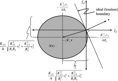
S(v) : Region of Feasible Forces, for a given velocity v

U(w) : Feasible forcing region for Nominal System Model, for a given state w

VS : DC bus voltage

Vswk : Switch conduction voltage for actuator k

VswR : Switch conduction voltage for dissipative interface

Z : Effective damping matrix for RFA network

ag : Ground acceleration

f,fk : Force vector with {f}k = fk = Total force of actuator k

fe, fek : Force vector with {fe}k = fek = Electromech. force for actuator k

fe* : Electromechanical force command

fmax, fkmax : Force vector with {fmax}k = fkmax = Rated force of actuator k

ik : Stator current for machine k

iSk : Current drawn from DC bus by actuator k

iSR : Current drawn from DC bus by dissipative interface

lk : Screw lead for actuator k

m : Number of actuators

n : Structural degrees of freedom

u , uk : Normalized force vector for Nominal System Model; i.e. fe = Cc1/2u

v , vk : Actuation velocity vector with {v}k = vk

x : Electrical system state vector

w : Normalized structural system state vector for Nominal System Model q : Structural displacements, relative to the ground

hk : Screw efficiency for actuator k

Chapter 1. Introduction

Growing attention in recent decades has been devoted to methods of active feedback control of buildings and bridges, to reduce their responses to earthquakes and winds.

Considerable effort has been directed toward the design of force actuators for these structures, the development of sensory technology, and the synthesis of feedback control laws customized for these types of applications. The resultant body of research devoted to these subjects is rich and vast (Fujino et al. 1996; Housner et al. 1997; Soong 1990; Spencer and Sain 1997; Spencer and Nagarajaiah 2003). Feedback control affords certain advantages in the context of earthquake engineering, which motivate the continually growing interest in this field. By using externally powered electrical or hydraulic devices to apply forces to structures, active forcing systems have been shown to greatly reduce the excitation of a building during seismic events, in comparison to simpler passive systems. Part of this improvement is due to the availability of external power, and part is due to the use of sensory systems to formulate control actions based on global structural deformation characteristics.

The first commercial building equipped with an active control system, designed by the Kajima Corporation in 1989, is the Kyobashi Center, located in Tokyo (Ikeda et al. 2001). Its control actuators consist of two hydraulic active mass drivers (AMDs) on the roof of the 11-story structure. Together, the weight of these masses is approximately 1% of the structural mass. One of these AMDs suppresses the lateral motion of the structure, while a secondary AMD suppresses torsional motion. The system was designed to reduce vibrations due to moderate winds. To date, this constitutes one of only four or five times that a fully active control system has been

successfully installed in a commercial building (although several more implementations have been successfully applied toward the stabilization of pylons during the erection of bridges). There are many reasons for the failure of this technology to gain a foothold in the industry, not the least of which is the associated cost. However, aside from expense, active structural control systems have two significant and fundamental disadvantages which diminish their likelihood of gaining acceptance in practice.

The most fundamental disadvantage of active control is that it in general requires an external power supply. This presents questions about both reliability and practicality. In civil engineering applications, an active control system designed to protect a building during

shown that during earthquakes, the power grid is highly susceptible to destabilization and blackouts. On the other hand, the power demands of active control systems for large buildings are typically too large to be met with local supplies. Thus, active control systems are, by their very nature, inherently unreliable.

The second disadvantage of active control is that, by designing an actuator which may accept power from an external source, the system cannot be characterized as a “bounded-energy” system. Questions therefore quickly arise concerning the stability-robustness of such systems. Although significant effort has been put toward alleviating this problem through the application of robust control theory, the nature of model uncertainty in civil engineering structures is such that significant concerns remain unresolved.

One compromise between active and passive actuation is found in hybrid systems. These consist of a combination of active and passive systems working in tandem. Hybrid systems are more reliable, because the passive part of the actuator will still work in the absence of power. Extensive research over several decades has yielded many different designs for these systems (Soong 1990) and to date over 40 commercial buildings in Japan alone, as well as many more in China, Taiwan, and Korea have been equipped with some form of hybrid actuation (Ikeda 2004; Spencer and Nagarajaiah 2003).

Another important emerging technology in structural control concerns low-power, high-performance force actuators called semiactive devices (Symans and Constantinou 1999). These devices are dissipative like passive devices, but possess fast-acting variable properties which may be “tuned” in real-time to optimize the dynamic response of the structure. Despite their

limitations, such devices exhibit some of the appealing traits of active systems, in that they are capable of real-time force control, although in a limited range. Also, the parameters of a semiactive device situated in one location in the structure may be controlled based on the dynamic response of the entire structure. The only power necessary for operation of semiactive systems is that which is needed for the sensors and control intelligence, and to tune the device parameters. Typically these demands are orders of magnitude below the power flow capabilities of the devices.

1.1: Semiactive Forcing Systems

x

g

f

f

f

g

x&

x

g

f

f

f

g

x&

Figure 1.1: Idealized semiactive damper

will be of a desired magnitude. This parameter corresponds to some property of the device which may be modified to yield the differing curves in Fig. 1.1.

Perhaps the simplest example of a real semiactive device is the variable-orifice damper. In this case, the parameter g represents the size of the orifice through which the viscous fluid in the damper is forced to flow, due to the motion of the piston. Theoretically, it requires no work to change the size of the orifice. Rather, the orifice size simply controls the amount of energy dissipated by the surrounding mechanical system. Therefore, if the device were ideal, there would be no power flow associated with parameter g. In actuality, of course, there is a small amount of work associated with g, because there will be losses in the electromechanical system which changes the orifice size, but these losses are extremely small, in comparison to the power flow of the actuator. This is a common trait of all semiactive actuators. Their control parameters do not have significant power flow associated with them. In fact, most semiactive devices, even ones which have force capabilities of over 10 tons, are capable of operating for extended periods of time using only a battery for a power supply.

Semiactive actuation has received a fair amount of attention during the last decade because of its potential for reliable, low-power structural control. There are two distinct advantages to semiactive control. The first of these is that, for a structure which is open-loop stable (i.e., stable without control), the implementation of a control system employing semiactive actuators physically cannot destabilize the structure. Thus, some questions concerning stability-robustness vanish. Secondly, semiactive actuators are unaffected by external power supply failures (as they operate on small, local, battery power) making them more reliable.

automotive suspensions, where they have exhibited favorable, reliable performance, while consuming negligible power.

1.1.1: Semiactive Control of Civil Structures: A Brief History

Semiactive devices were first researched in the area of vehicular suspensions over twenty-five years ago (Croila and Abdel-Hady 1991; Karnopp et al. 1974). In civil engineering, interest in these devices is a more recent phenomenon (Patten et al. 1994; Spencer 1996). There have been many different types of semiactive devices proposed for civil engineering structures. The following is a short list of some of these investigations. It is not intended to be a complete, exhaustive listing of the many contributions in this area. For more thorough surveys, see (Spencer and Nagarajaiah 2003) and (Housner et al. 1997).

· Variable Orifice Fluid Dampers: In the civil engineering area, the ability of variable-orifice dampers to reduce the response of buildings subjected to seismic loads has been shown to be effective (Hrovat et al. 1983; Kurata et al. 1994; Liang et al. 1995; Mirzuno et al. 1992; Patten et al. 1994; Sack et al. 1994; Shinozuka et al. 1992; Symans and Constantinou 1996; Symans et al. 1994). These results have concerned simulation and small-scale experiments. In addition, some full-scale experiments have also been done for a building (Kamagata and Kobori 1994; Kobori et al. 1993) and for a bridge (Feng and Shinozuka 1990; Kawashima et al. 1992).

· Controllable Tuned Liquid Dampers: Normal tuned liquid dampers dissipate energy through the sloshing of a fluid in a tank, which is excited by the structure. The fluid, and tank, are designed such that the sloshing effect resonates near the resonant frequency of the structure. Several studies (Kareem 1994; Lou et al. 1994; Yalla and Kareem 2003; Yeh et al. 1996) have been conducted which equip these dampers which semiactive characteristics.

· Variable Stiffness Devices: The idea of using a variable-orifice damper as an on/off variable-stiffness device was first proposed by (Kobori et al. 1993). Since that time these researchers, and others at the Kajima Corporation in Japan, have developed the concept into a commercially-viable technology, which has been implemented in numerous buildings over the last decade (Kobori 2003; Yamada and Kobori 2001). Various methods of structural control have been developed for these devices (Nasu et al. 2001). One particular approach (Hayen and Iwan 1994), in which the main structure is interfaced with one or more secondary structural systems.

A device capable of continuously varying its stiffness has been proposed by (Nagarajaiah and Mate 1998). Such a device may be characterized as semiactive, because the amount of power needed to vary this stiffness can be made much lower than the overall power flow of the stiffness system. This device has been implemented in the capacity of a scale-model controllable TMD.

· Controllable Fluid Dampers: Controllable fluid dampers possess fluids with properties which may be influenced by the presence of magnetic or electric fields. For these two cases, the dampers are called magnetorheological (MR) and electrorheological (ER) dampers. Rheological fluids (both kinds) were discovered in the 1940’s (Rabinow 1948; Winslow 1947; Winslow 1949). When the respective fields are applied to these fluids, their behavior changes from that of a low-viscosity fluid to more of a semi-solid, visco-plastic behavior. Thus, the application of such a fluid in a damper gives the ability to actively control the effective viscosity of the damper through electrical and magnetic fields. Research on ER fluids has been quite extensive. ER fluid dampers have been shown to be quite effective in civil engineering applications, as evidenced in (Ehrgott and Masri 1992; Ehrgott and Masri 1994a; Ehrgott and Masri 1994b; Gavin et al. 1994a; Gavin et al. 1994b; Gordaninejad et al. 1994; Leitmann and Reithmeier 1993; Makris et al. 1995; Masri et al. 1995; McClamroch and Gavin 1995). Recent research in MR fluid dampers has demonstrated their use in the

Dyke et al. 1996b; Dyke et al. 1996c; Spencer et al. 1996; Spencer et al. 1997). In addition, a 20-ton MR damper, discussed in (Carlson and Spencer 1996) and (Spencer et al. 1997), demonstrates that these devices can be scaled for civil engineering applications.

Semiactive devices are beginning to be implemented in commercial applications in Japan by the Kajima Corporation. Notable among these implementations are four new buildings in the Siodome area of Tokyo, including the 38-story Siodome Tower, which have been designed with switching hydraulic dampers and feedback control systems. Also, the 54-story Mori Tower, in the Roppongi area of Tokyo, has over 350 variable-orifice dampers installed.

1.1.2: Electromechanical Dissipation

All of the semiactive devices thus far described dissipate energy through mechanical means. For instance, the variable-orifice and the controllable fluid dampers dissipate energy as liquid passes through an orifice. Likewise, the variable friction damper dissipates energy at the contact surface. However, energy may also be dissipated through electrical means. For instance, in the control of flexible structures with piezoelectric materials, research has shown that

considerable reduction in vibration can be accomplished by the application of electrical RL shunt impedances across the terminals of the piezoelectric actuator (Hagood and von Flotow 1991). Such impedances store, and dissipate, electrical energy transduced by the piezoelectric material from the vibrating structure. Such ideas were expanded to a semiactive framework by allowing the resistor to be controllable in real time, with favorable results (Edberg and Bicos 1991; Hollkamp and Starchville 1994). This idea constitutes a kind of semiactive control.

For civil engineering applications, the same concept may be applied. However, because of the physical scale of civil structures, the piezoelectric materials used in lightweight, flexible aerospace structures cannot be employed. Instead an electric motor, by operating as a generator, could be used to convert mechanical to electrical energy. Then, this energy could be dissipated in an electrical network. This idea has been applied to semiactive vehicle suspension design by Karnopp (1989). Semiactive control through electrical dissipation has an advantage over mechanical methods in that such devices may also be operated as active devices if power is available. A semiactive device which uses an electric motor to facilitate energy dissipation may be driven as an active device by a simple switch in the circuitry to which the machine is

w

rotor shaft

stator coils stator

permanent magnets

i_a

i_a

A

A'

C

B' C'

w

rotor shaft

stator coils stator

permanent magnets

i_a

i_a

A

A'

C

B' C'

Figure 1.2: A permanent magnet brushless DC machine (cutaway)

A study by Nerves and Krishnan (1996) concluded that the optimal electromechanical actuator for use in civil structures is the permanent-magnet brushless DC (PMBDC) machine. Such a machine is shown in Fig. 1.2. Mounted to the rotor of the machine are permanent magnets which provide a rotating magnetic field as the rotor spins. The interaction of this magnetic field with the stator windings provides the avenue by which mechanical power on the machine shaft is converted to electrical power in the stator coils, and vice versa. Currently, these machines are available commercially at power ratings in excess of 20kW, placing them in the right “ballpark” for civil structure applications.

In Scruggs and Iwan (2003), these machines are used in the design of semiactive electromechanical devices for use in civil structures. A basic schematic for such a device is illustrated in Fig. 1.3. This conceptual diagram shows a rotational electric motor being used as a linear force actuator, by means of a linear-to-rotational converter consisting of a gear reduction and screw mechanism. Two electrical circuits may be connected to the motor, depending on the

V+_{_}

linear / rotational conversion

electric motor

active circuitry

semiactive

circuitry R

i f, v

stator currents

active circuitry used when external power supply voltage

Vis available. Otherwise, switch to semiactive circuitry.

i_a i_b i_c torque and

angular velocity linear force

and velocity

T, wr

V+_{_}

linear / rotational conversion

electric motor

active circuitry

semiactive

circuitry R

i f, v

stator currents

active circuitry used when external power supply voltage

Vis available. Otherwise, switch to semiactive circuitry.

i_a i_b i_c torque and

angular velocity linear force

and velocity

T, wr

+

-V_g

V_g<V_off V_g>V_on

+

-V_g

V_g<V_off V_g>V_on

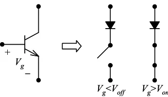
Figure 1.4: Operation of the transistor as an electrical switch

positions of three switches. The upper, “active” circuitry is connected to an external power source, and may be designed to actively drive the force actuator. When the switches are in the "down" position, the motor is connected to the "semiactive" circuitry, consisting of a network of passive components (i.e., resistors, inductors, etc.) and transistors.

In the semiactive mode of operation, the device uses the motor as a generator which converts mechanical energy to electrical energy, which in turn is dissipated in the network. By controlling the transistors in the network, this energy dissipation can be regulated, using concepts from basic power electronics (Kassakian et al. 1991). The transistors are used as “electronic switches,” as illustrated in Fig. 1.4. By proper selection of the voltage Vg, the transistor

resembles a mechanical switch in parallel with a diode. As with actual mechanical switches, this mode of operation consumes very little power, even if the electric power flowing through the network is very high. As these transistor switches (together with the sensors and control

intelligence) constitute the only demand for an external power source, the system is semiactive. In Scruggs and Iwan (2003), it was shown that the performance of such an

electromechanical semiactive device is competitive with that of a similar-sized

magnetorheological fluid damper, and that the rotational inertia of the device actually works to the benefit of the overall system performance.

1.2: Regenerative Force Actuation

In the last decade a separate class of actuator, first formally defined by Jolly and Margolis (1997a), has been proposed for use in structural control. Called Regenerative Force Actuation

flow capabilities. However, they have two characteristics which set them apart from semiactive devices:

1) Power storage and reuse: Semiactive devices must always remove energy from the mechanical system. By contrast, RFA systems have the capability of storing at least a fraction of the energy they remove from the mechanical system, and of re-injecting that energy back into the mechanical system at a later time.

2) Power coupling in actuation networks: When multiple regenerative actuators are distributed throughout a structure, they may be capable of “sharing” power with each other. For

example, one device may remove energy from a mechanical system from one location, while another device simultaneously re-injects that energy back into the mechanical system at another location.

The advantage of RFA systems is that they, like their semiactive cousins, are a compromise between active and passive designs. Many of the favorable power and reliability issues of semiactive actuators extend to regenerative ones. However, regenerative actuators relax the constraints imposed on semiactive systems, giving these devices the potential to “push the envelope” for the level of performance achievable for energy-constrained control.

The concept of regenerative actuation have appeared in numerous areas of structural control, and there exist some differences as to exactly what qualifies an actuation system as “regenerative.” These discrepancies arise from how the energy storage system is modeled (if it is included at all), whether multiple actuators are considered, and if so, whether they are allowed to share power. In this section, a brief synopsis of some past contributions on this subject will be presented. Then, the framework in which these devices will be considered for this study will be presented. This framework is intended to be rather general, in the sense that it applies to systems with or without energy storage, and to arbitrarily large actuation networks.

1.2.1: Past Work

linear / rotational conversion

electric motor T, w

f, v

stator currents

i_a i_b i_c torque and

angular velocity linear force

and velocity

electronic drive circuit

+

–

V_S i_S

S S’ linear /

rotational conversion

electric motor T, w

f, v

stator currents

i_a i_b i_c torque and

angular velocity linear force

and velocity

electronic drive circuit

+

–

V_S i_S

S S’

Figure 1.5: Block diagram of an actuator subsystem

In the area of vehicle suspensions, regenerative actuators are defined in (Jolly and Margolis 1997a; Jolly and Margolis 1997b) as a network of force actuators which has power-coupled capability (i.e., trait 2 above) and which possesses a single, global, ideal energy storage device. By “ideal,” the implication is that this storage device possesses no dynamics, has 100% efficiency, and has no upper limit on energy capacity. In that study, both electrical and hydraulic designs are discussed. The emphasis is on steady-state disturbance rejection problems, and the energetic constraints of the devices are handled by classifying linear feedback control laws for which, in steady-state or stationary excitation, the energy stored in the power supply tends to infinity.

In civil engineering applications, regenerative actuators have received much less

attention. Nerves and Krishnan (1996) conducted investigations into this subject where, as in the aforementioned suspension research, this power supply is considered to be ideal. A study

conducted by Scruggs (1999) examined the implications of the fact that the energy storage system has a limited size, resulting in saturation and exhaustion of the supply system. It is also important to mention that in the civil engineering area, studies with regenerative actuators have been limited to a single device with local energy storage. The concept of power-sharing between actuators has yet to receive any significant attention.

1.2.2: A Generalized Approach

The concept of regenerative actuation can be approached as an extension of the electromechanical semiactive system discussed in the previous section. Consider again the system depicted in Fig. 1.3, slightly revised in Fig. 1.5. If terminals S-S’ are connected to an energy source instead of a resistor, the system in Fig. 1.5 is capable of two-way power flow. The present study envisions the use of several such electromechanical systems (henceforth called

actuator subsystems) as force actuators for use in structural vibration control. With the terminals

2

1

a

1

2

b

3

1 2

c

2

1

a

2

1

a

1

2

b

1

2

b

3

1 2

c

3

1 2

c

Figure 1.6: Various Applications of Regenerative Actuation

power with each other, through proper control of the electrical circuitry. Thus, the electrical energy generated by one device may be converted back into mechanical energy by another.

Remote energy storage and reuse is possible for this system. The simplest way to accomplish this is by designing one of the actuation subsystems as a flywheel drive system. Thus, the energy storage device becomes just another degree of freedom in the mechanical system to which the RFA system is connected. If an energy supply does not exist, or if it is saturated at its maximum storage level, excess electrical energy may be dissipated in a resistor bank, also connected to S-S’.

In this context, RFA systems have many potential uses in the control of civil structures. Consider, for example, the possible implementations shown in Fig. 1.6. In Fig. 1.6a, two machines are incorporated into a structure, one between the ground and first floor, and the other in the form of a mass driver on the roof. If machine 1 were operated as a generator and machine 2 as a motor, the system could deliver energy directly from the ground to the roof. Or, as shown in Fig. 1.6b, one of the two machines could be mounted on the ground and made to drive a flywheel using energy withdrawn by the second machine. In this way, machine 1 is used as an energy storage device. Yet another possible configuration is the densely-actuated structure in Fig. 1.6c. The capability of the actuators to share power allows for the structural vibration energy to flow in more complex patterns than for traditional damping systems.

1.2.3: The Ideal RFA Network

DC bus

f₁, v₁

f₂, v₂

f_m, v_m

mechanical

system

machine subsystem m

machine subsystem 2

machine subsystem 1

i_S1

i_S2

i_Sm

dissipative interface

+ –

V_S C_S R_S iSR iR R_R

DC bus

f₁, v₁

f₂, v₂

f_m, v_m

mechanical

system

machine subsystem m

machine subsystem 2

machine subsystem 1

i_S1

i_S2

i_Sm

dissipative interface

+ –

V_S C_S R_S iSR iR R_R

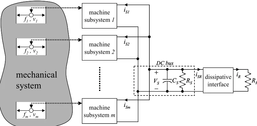
Figure 1.7: Idealized Electromechanical Regenerative Actuation System

and the corresponding relative velocity vector is v = {v1...vm}T. For each actuator, the power

injected into the structure is Pk = fekvk. This mechanical power is converted from an electrical

power VSiSk. Ideally, this power conversion would be lossless and instantaneous, with fekvk being

equal to VSiSk. The terminals S-S’ of all the machines are connected in parallel, and referred to as

the DC bus, with voltage VS. Also connected to the DC bus is a “dissipative interface” which is

used to dissipate excess electrical energy generated by the actuators. This subsystem extracts current iSR from the DC bus, to produce a current iR through resistor RR. Ideally, the dissipative

interface would be lossless and instantaneous, with VSiSR equal to iR2RR.

As with the electromechanical semiactive device discussed in the previous section, this electrical network (i.e., inside the boxes labeled “electronic drive circuit” in Fig. 1.5 and

“dissipative interface” in Fig. 1.7) is controlled by using transistors as electronic switches. Thus, ideally, control of these electronic networks consumes negligible power.

In Fig. 1.7, capacitor CS is not intended to store any significant amount of energy, and

resistor RS is selected to be sufficiently large, such that the energy it dissipates is minimal.

Therefore, in ideal steady-state operation, the aggregate power flow onto the DC bus is approximately zero, implying that

R R m

k S

SkV i R

i 2

1

-=

å

=

(1.1)

0 1

£

å

= m

k S SkV

i (1.2)

Lossless power conversion further requires that iSkVS = fekvk so the above leads to the ideal

regenerative actuation constraint,

0 1

£ =

å

=

v

fT

e m

k k ekv

f (1.3)

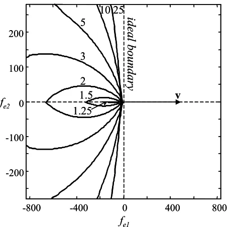
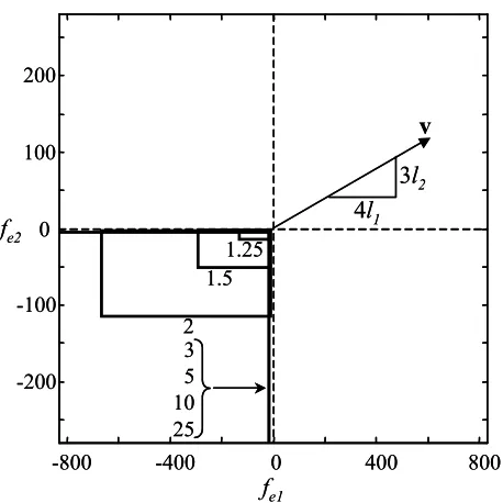
For an ideal RFA network, the above relationship is the only constraint on the forces. Of course, the power conversions in a real electromechanical system are not lossless. The electrical system also possesses significant dynamics and limitations which must be modeled. These issues constrain the system operation, producing realistic regenerative actuation constraints that are more restrictive and complex than the one in equation (1.3). However, the above discussion illustrates the general concept of regenerative actuation.

1.3: Objectives & Scope of This Study

The focus of this study concerns the design, modeling, simulation, and control of RFA networks, such as the one in Fig. 1.7, and their implementation in structural control problems pertaining to earthquake engineering. The ensuing chapters delve deeper into these concepts, following the outline below:

Ch.2: System Modeling. The design of a realistic RFA network, with arbitrary number of actuators and possible energy storage, is developed. This leads to a physical model for the electrical dynamics of the RFA network, in which the inputs to the system are the linear velocity vector v, and the positions of the electronic switches in the network. Ch. 3: Capabilities of RFA Systems. The theoretical forcing capability of the designed RFA

network is examined, yielding a single constraint similar to Eq. (1.3), but accounting for internal electrical losses in the network, and practical limitations on the electrical states. Implications for systems with power storage are examined, which paint a more complex picture of the energy storage capability of these systems than the “ideal” supply

assumptions of previous studies.

robust to parameter uncertainties and sensory time delay. The transient characteristics of the closed-loop system are also examined.

Ch. 5: The Structure-Actuator System. The integration of the RFA network into a linear structural model is presented. Also, a “nominal model” of the actuator-structure system, for use in the design and analysis of the structural feedback controller, are presented. It is then shown that the RFA network may be viewed as a structural damping system, but where the damping capabilities are more general than those achievable with mechanical damping. For instance, the damping forces may be non-local, and the resultant structural damping matrix may be asymmetric. Scalar measures are defined, by which the

performance of the RFA structural control system may be assessed, and these measures are used to optimize the linear damping for the RFA network.

Ch. 6: Feedback Control Algorithms. The development of “Clipped-Linear” feedback control is presented. This approach to controller design is common for semiactive devices, and has been shown to yield favorable performance. Here, it is extended to RFA networks, and several simple examples are given which examine its performance. Its equivalence to Lyapunov-based control system design is also discussed.

Ch 7: A Simulation Example. For the control system design approaches developed in Chapter 6, a numerical example is shown which exhibits the performance of an RFA network for the actuator configuration shown in Fig. 1.6a, subject to earthquake loading. The performances of several feedback controller designs are compared to each other, and to the uncontrolled case. Characteristics arising from the non-ideal network realization are illustrated.

Ch. 8: Optimal Control. The constraints on the RFA network result in a physical limitation on the achievable performance for the system. The derivation and study of this physical limit is useful in the design of RFA networks for particular applications. This chapter presents some ideas on the use of optimal control theory to derive this performance limit. However, there are basic questions in this analysis which remain unanswered, and

consequently, the results presented here are merely preliminary.

Ch. 9: Conclusions and Future Research. Conclusions are drawn for this study, and the numerous avenues for future research are discussed.

in this analysis that the designs presented herein are optimal for a given application, or that they represent concepts which could be carried directly into practical implementation without modification or refinement. Rather, an effort was made to strike a comfortable balance between theoretical tractability and technological realism.

Chapter 2. System Modeling

The RFA network in Fig. 1.7 is quite general. It is not stated how the electromechanical conversion is accomplished in each actuator subsystem, or how the current iR is regulated through

the dissipative interface. This chapter constitutes one description of how such an RFA network might be constructed, along with a derivation of a dynamic model of its behavior.

For each actuator in the network, the proposed design of the actuator subsystem is shown in Fig. 1.5. The linear-to-rotational conversion converts the linear force fk to a torque Tk. The

machine converts the mechanical energy to electrical energy, and vice versa. Finally, the power electronics interface the terminals of the machine with the DC bus. This system has nontrivial dynamic behavior due to dissipation, inductances in the stator coils, etc. The DC bus subsystem also has dynamics, because of its capacitance CS. Its inputs are the currents from the machine

subsystems and the dissipative interface. The dissipative interface subsystem has dynamic behavior as well, and must be controlled to properly regulate the current iR flowing through its

resistor.

The approach of this chapter is to model and discuss each subsystem in Fig. 1.7 (i.e., the actuator subsystems, DC bus, and dissipative interface) separately. For each, its hardware design will be presented, and its dynamic model derived. Then, at the end of the chapter, the dynamic description of the entire network is presented.

2.1: The Actuator Subsystems: Electromechanical Conversion

All actuator subsystems are assumed to be assembled from the same types of

components; i.e., the same types of linear-to-rotational conversions, motors, etc. However, these components may have different parameters for each subsystem. As they all obey the same fundamental laws, their descriptions may be generalized. For convenience, the notation of subsystem number (i.e., fek) will be dropped (i.e., fe) with the tacit implication that such

expressions apply to all the subsystems in the network.

2.1.1: Mechanical Modeling

w

l

v= (2.1)

where l, called the lead of the conversion, has units of m/rad. For the purposes of this analysis, the efficiency of the screw conversion will be considered the same in both directions of operation, and will be denoted by h. Other attributes of the conversion, such as backlash and axial play, are considered negligible in this analysis.

The shaft torque T is related to the linear force f through the lead and the efficiency. For convenience, define h(Tw) as

( )

£ ³ =

0 :

1

0 :

w h

w h

w

T T T

h (2.2)

Then f can be expressed as

( )

l T h

f = w (2.3)

Note that h(Tw) is equal to h(fv).

For machines in the network used to excite flywheels, there is obviously no linear-to-rotational conversion. However, it will be inconvenient to continually make distinctions between linear and rotational actuators in the mechanical system. Thus, flywheels will be incorporated into the general framework by designating h=1 and choosing an arbitrary l for these subsystems. Unless otherwise stated, no distinction will be made between these and other actuator subsystems.

b

a b

c a’

b’

c’

N

S

v_bn a

c n +

-v_an +

-v_cn

-+

b

a b

c a’

b’

c’

N

S

v_bn a

c n +

-v_an +

-v_cn

-+

Figure 2.1: Cross-section of a BDC machine

The angular velocity of the rotor shaft is denoted by w, and the resultant angular

displacement is q. Let the torsional viscous friction coefficient and rotational inertia of the rotor be denoted by B and J, respectively. Then, the resultant total torque T transmitted to the shaft may be expressed as

w

w B

J T

T= _e - & - . (2.4)

Defining fe as

l T

fe= e/ (2.5)

the mechanical dynamics of the machine can be described in terms of the linear motion variables as

( )

ø ö çç

è æ

-= v

l B v l

J f fv h

f _{e 2} & ₂ . (2.6)

In the ensuing analysis, it will be convenient to work directly with fe rather than f, with the

understanding that they are related through Eq. (2.6).

2.1.2: Electrical Modeling

neutral node, labeled as n. The corresponding line-to-neutral voltages applied to the terminals are

van, vbn, and vcn.

With the stator coils connected as described, the electrical dynamics of the stator currents may be represented by the equivalent circuit shown in Fig. 2.2. For instance, the a-phase current

ia satisfies the differential equation

dt di L Ri e

v a

a an

an = + + (2.7)

In the figure, R and L are the resistance and effective inductance, respectively, for each stator coil. The equivalent voltage sources ean, ebn, and ecn, called the back EMF voltages, result from

magnetic induction between the rotor and stator fields. These voltages are related to the

mechanical dynamics of the rotor. Through its angular velocity and position, this relationship is described by the periodic, trapezoidal functions Ka, Kb, and Kc, shown in Fig. 2.3. Using these

functions, ean is

( )

a an K

e = (2.8)

Analogous expressions follow for the b and c phases.

The electromechanical force fe, due to the stator currents, can be found by equating the

electrical power flow iaean+ibebn+icecn (into the back EMF voltages) to the resultant mechanical

power delivered by the actuator, equal to fev. This gives

(

)

(

)

cn c bn b an a e

i K i K i K l

v e i e i e i f

+ + =

+ + =

1 (2.9)

where Ka, Kb, and Kc become functions of linear displacement, through parameter h. With fe thus

defined, Eqs. (2.1) through (2.9) fully describe the dynamics of each actuator subsystem.

n

R L

i_a

a

R L

i_b

R L

i_c

b

c

+ v_an –

+ –e_an

+ –e_cn + –e_bn

+ v_cn – + v_bn –

n

R L

i_a

a

R L

i_b

R L

i_c

b

c

+ v_an –

+ –e_an

+ –e_cn + –e_bn

+ v_cn – + v_bn –

-K₀ 0 K₀

0

0 -K₀ K₀

-K₀ K₀

0 p/6 p/2 5p/6 7p/6 3p/2 11p/62p

AR1 AR2 AR3 AR4 AR5 AR6 AR1

q_r

K_a

K_c K_b

-K₀ 0 K₀

0

0 -K₀ K₀

-K₀ K₀

0 p/6 p/2 5p/6 7p/6 3p/2 11p/62p

AR1 AR2 AR3 AR4 AR5 AR6 AR1

q_r

K_a

K_c K_b

Figure 2.3: Trapezoidal back-EMF functions

2.2: The Actuator Subsystems: Electronic Conversion

The objective is to use the machine as a force actuator; i.e., to excite currents ia, ib, and ic

in such a way that fe tracks some desired force fe*. By Eq. (2.9), this implies that the three stator

currents have to be controlled to track a set of commands ia*, ib*, and ic* such that

(

)

c c b b a a

e K i K i K i

l

f = + + (2.10)

However, there are three currents, and one desired force, so Eq. (2.10) is not enough to determine three unique current commands (i.e., the problem is overdetermined). Two additional,

independent relations for the current commands are necessary.

One of these relations is immediate. Because the three coils connect at the neutral node

n, the currents must always sum to zero. Therefore, for successful current tracking, it must always be the case that

0 * *

* _{+ + =}

c b a i i

i (2.11)

The other relation arises from convenience rather than necessity. Consider again the trapezoidal back-EMF waveforms in Fig. 2.3. Define a current command i* _{to be related to the}

three stator current commands as shown in Fig. 2.4 below. Note that this set of current commands always meets Eqs. (2.10) and (2.11). Defined as such, Eq. (2.10) becomes

* * _{K i}

0 i*

0

0

0 p/6 p/2 5p/6 7p/6 3p/2 11p/62p

AR1 AR2 AR3 AR4 AR5 AR6 AR1

q_r

i_a*

i_c*

i_b*

-i*

i*

-i*

i*

-i*

0 i*

0

0

0 p/6 p/2 5p/6 7p/6 3p/2 11p/62p

AR1 AR2 AR3 AR4 AR5 AR6 AR1

q_r

i_a*

i_c*

i_b*

-i*

i*

-i*

i*

-i*

Figure 2.4: Current commands

where

l K

Kf =2 0/ (2.13)

Eq. (2.12) is convenient because the relationship between fe* and i* is proportional and

time-invariant. Through Fig. 2.4, it determines uniquely the current commands ia*, ib*, and ic* as a

function of fe*. It is also an l¥-optimal solution to Eqs. (2.10) and (2.11) for {ia*,ib*,ic*}, and thus

yields the maximum amount of force for a given current level.

2.2.1: Drive Circuitry

The drive circuitry is an electronic network connected to the terminals of the machine that provides the means of controlling the stator currents. It interfaces the machine terminals with the DC bus voltage VS, as was shown in Fig. 1.5.

Terminals a, b, and c are connected to a six-transistor drive circuit which interfaces with

VS, as shown in Fig. 2.5. The dynamics of the circuit are influenced by the on/off switching

ability of the transistors. By firing the transistors on and off, the stator currents can be raised and lowered. Thus, by proper concurrent timing of these firings, the currents can be controlled.

In order to render a tractable model for the electrical dynamics, the traits of the transistors and diodes will be approximated. The diodes are modeled by a nonzero forward conduction voltage VD and infinite reverse breakdown voltage.

Because they are operated as electronic switches, the transistors can be approximated as in Fig. 2.6, where Vgs is the gate-source voltage, used to switch the transistor “on” and “off.” The

T4 T6 T2 T5 T3

T1

n

R L

i_a

R L

i_b

R L

i_c + –e_an

+ –e_cn

+ –e_bn +

–

VS

iS

motor

a

b

c

T4 T6 T2

T5 T3

T1

n

R L

i_a

R L

i_b

R L

i_c + –e_an

+ –e_cn

+ –e_bn +

–

VS

iS

motor

a

b

c

Figure 2.5: Transistor bridge

on and off requires very little current ig, even if the current ids is quite large. As a result, the gate

drive circuitry which excites the voltage Vgs typically consumes very little power.

Fig. 2.6 is an approximate model. Among other characteristics, it ignores dissipation which occurs as the transistor turns on and off.

With the transistor approximation in Fig. 2.6, the transistor bridge circuitry may be approximated by the switching system in Fig. 2.7.

2.2.2: H-Bridge Switching Logic

A system of control logic must be determined for these transistors in order to control the stator currents so as to track the commands illustrated in Fig. 2.4.

Consider that for any rotor angle q in Fig. 2.4, one stator current command is always zero. Suppose that at some time t, q(t)ÎAR1. Thus, ia*=0. Under the condition that

) ( )

(t K vt

VS > f (2.14)

for t>t, the current ia(t) = 0 is a stable equilibrium point if neither transistor T1 or T4 is activated.

Thus, it is possible to achieve tracking for the zero-current phase by not firing either of its corresponding transistors.

+ – V_gs

g

s

d d

s Vgs<Voff(approx. and actual) Vgs>Von(actual)

Vds

ids

VT

0

Vgs>Von(approximate)

+ – V_gs

g

s

d d

s Vgs<Voff(approx. and actual) Vgs>Von(actual)

Vds

ids

VT

0

Vgs>Von(approximate)

n

R L

i_a

R L

i_b

R L

i_c + –e_an

+ –e_cn

+ –e_bn +

–

VS

i_S

motor

a

b

c _{T4 T6 T2}

T3

T1 T5

n

R L

i_a

R L

i_b

R L

i_c + –e_an

+ –e_cn

+ –e_bn +

–

VS

i_S

motor

a

b

c _{T4T4 T6T6 T2T2}

T3 T3 T1

T1 T5T5

Figure 2.7: Approximate transistor bridge

If q ÎAR1 for all time, the schematic in Fig. 2.5 can then be simplified by removing the

a-phase circuitry, because it is known that ia = 0. Similarly, if q ÎAR4 for all time, the simplified

schematic would look the same. Furthermore, for q in any angle range for all time, the resultant schematics differ only in their transistor assignments. The schematic Fig. 2.8 could then be used to accurately model its behavior, by keeping track of which transistors T1-T6 assume the roles of T1S, T2S, T3S, and T4S in the various angle ranges, as shown in the accompanying table. The relationships between i and the actual stator currents ia, ib, and ic also differ for different angle

ranges. The relationships of these three currents to i, for all six angle ranges, are the same as for the current commands shown in Fig. 2.4. The relation of i to the force fe is therefore also the

same, i.e.,

i K

f_e= _f (2.15)

The operation of the 6-transistor drive in Fig. 2.5 follows from this rationale. For q in a given angle range, four of the transistors take on the roles of T1S through T4S, while the other

1S 2S 3S 4S i=

AR1 5 2 3 6 ic, -ib AR2 1 4 3 6 ia , -ib AR3 1 4 5 2 ia , -ic AR4 3 6 5 2 ib , -ic AR5 3 6 1 4 ib , -ia AR6 5 2 1 4 ic , -ib

2R 2L

i_c, -i_b

+

– K_fv

i_S

– V+_S

T1_S

D1_S D3_S T3_S

T6_S D6_S

T2_S D2_S

1S 2S 3S 4S i=

AR1 5 2 3 6 ic, -ib AR2 1 4 3 6 ia , -ib AR3 1 4 5 2 ia , -ic AR4 3 6 5 2 ib , -ic AR5 3 6 1 4 ib , -ia AR6 5 2 1 4 ic , -ib

2R 2L

i_c, -i_b

+

– K_fv

i_S

– V+_S

T1_S

D1_S T1_S

D1_S D3D3_SS T3T3_SS

T6_S

D6_S T6_S

D6_S T2_S

D2_S T2_S

D2_S

two (corresponding to the zero-current phase) remain switched off. When q transits from one angle range to another, these transistor assignments change.

After such a transition, one stator coil will demagnetize (i.e., its current will drop to zero) and another one will become activated. For example, a transition from AR1 to AR2 results in ib

dropping to zero and ia rising to i. Because of the inductance of the stator coils, this

magnetization/demagnetization process is not instantaneous, but rather occurs over a brief time period following the transition. These dynamics are not reflected in Fig. 2.8, and result in a pulsation in i during the transition. This phenomenon (which is the electrical equivalent of the mechanical commutation of the rotor in a traditional DC motor) will be considered negligible in this analysis. It has been shown elsewhere that its effect is so minimal in similar applications, and its inclusion greatly complicates the dynamic system description. Thus, Fig. 2.8 will be used as the dynamic model of the actuator subsystem.

The simplified 4-transistor bridge shown in Fig. 2.8 is called an H-Bridge, because of its geometrical shape. This type of motor drive is very common, and there exist several variations in the methods by which transistors T1S through T4S are used to control the currents. Here, only one of these is illustrated.

Consider the case where the current i satisfies

( )

Ri v K

VS > f +2 + swsgn (2.16)

where

T D sw V V

V = + (2.17)

If this inequality holds, then the circuit in Fig. 2.8 is equivalent to the one in Fig. 2.9, if the switch position S1 related to T1S and T2S by

i S1 T1S T2S >0 1 on off >0 2 off off <0 1 off off <0 2 off on

and if S2 is related to T3S and T4S by an analogous relationship.

2R 2L

i

+

–

K_fv

i_S

–

V

+

1 2

1 2

S1

S2

V_sw V_sw

2R 2L

i

+

–

K_fv

i_S

–

V

+

1 2

1 2

S1

S2

V_sw V_sw

V_sw V_sw

Figure 2.9: Approximate ideal-switch circuitry

î í ì

= =

-= =

=

1 S2 2, S1 : 1

2 S2 1, S1 : 1

D (2.18)

With this definition, the differential equation for the current i may be written as

(

)

2 1

i V Ri v K DV L i dt d

sw f

S - -

-= (2.19)

or, using Eq. (2.15),

( )

(

)

e K DV K v Rf K V f

L f dt

d

sgn 2

2

1 ₂

-= (2.20)

If Eq. (2.16) is true, then for D = 1, dfe/dt is positive and for D = -1, it is negative. Thus,

fe can be raised or lowered through these switches, and through proper alternation of D, its value

may be made to track a command fe*.

Eqs. (2.6) and (2.20) constitute a reasonable dynamic model for an actuator subsystem, under the assumption that VS satisfies Eqs. (2.14) and (2.16). In developing a switching control

algorithm for the RFA network, VS must be explicitly controlled to ensure that these conditions

are satisfied.

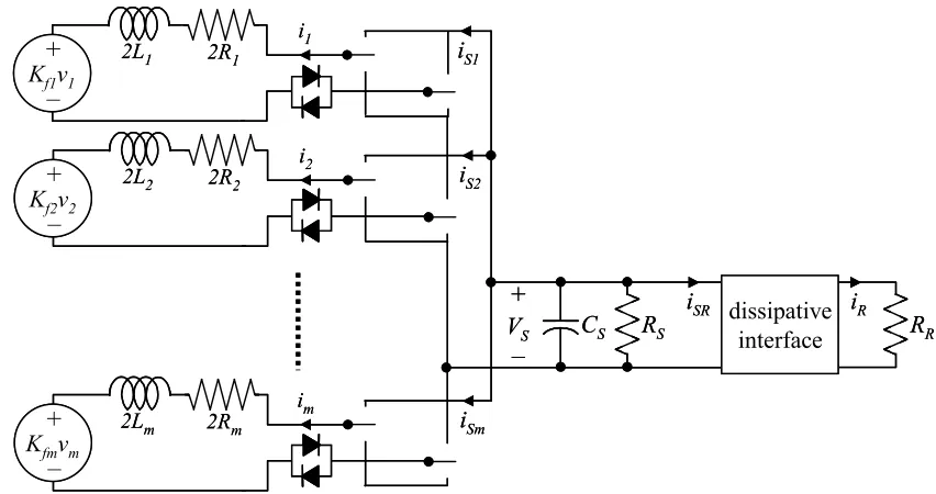
2.3: The Electrical Network

The various machines in the network are connected, both to each other and to the dissipative interface, through the voltage VS. This is shown in Fig. 2.10, assuming the general

case of m machines. This electrical bus is called a DC link, to imply that the voltage VS is a DC

i_S1 i_S2 i_Sm dissipative interface

+

–

V_S C_S iSR iR R_R

2R₁ 2L₁

+

–

K_f1v₁

i₁

2R₂ 2L₂

+

–

K_f2v₂

i₂

2R_m 2L_m

+

–

K_fmv_m

i_m R_S i_S1 i_S2 i_Sm dissipative interface

+

–

V_S C_S iSR iR R_R

2R₁ 2L₁

+

–

K_f1v₁

i₁

2R₂ 2L₂

+

–

K_f2v₂

i₂

2R_m 2L_m

+

–

K_fmv_m

i_m

R_S

Figure 2.10: Machine interconnections

network to another. The purpose of the capacitor CS is to filter out high-frequency voltage noise

which arises due to the switching of the transistor bridges. The resistor RS is present to provide

some light damping to the dynamics of the voltage VS. It is designed to be large, and typically

dissipates much less energy than RR.

The differential equation for VS may be expressed as

÷ ø ö ç è æ_{- - - -} -= S S SR Sm <