HIGHLIGHTED ARTICLE
| INVESTIGATION
Statistical Methods for Testing Genetic Pleiotropy
Daniel J. Schaid,*,1Xingwei Tong,†Beth Larrabee,* Richard B. Kennedy,‡Gregory A. Poland,‡ and Jason P. Sinnwell* *Department of Health Sciences Research and‡Mayo Clinic Vaccine Research Group, Mayo Clinic, Rochester, Minnesota 55905, and†School of Statistics, Beijing Normal University, 100875 Beijing, China
ABSTRACTGenetic pleiotropy is when a single gene influences more than one trait. Detecting pleiotropy and understanding its causes
can improve the biological understanding of a gene in multiple ways, yet current multivariate methods to evaluate pleiotropy test the null hypothesis that none of the traits are associated with a variant; departures from the null could be driven by just one associated trait. A formal test of pleiotropy should assume a null hypothesis that one or no traits are associated with a genetic variant. For the special case of two traits, one can construct this null hypothesis based on the intersection-union (IU) test, which rejects the null hypothesis only if the null hypotheses of no association for both traits are rejected. To allow for more than two traits, we developed a new likelihood-ratio test for pleiotropy. We then extended the testing framework to a sequential approach to test the null hypothesis thatk11 traits are associated, given that the null ofktraits are associated was rejected. This provides a formal testing framework to determine the number of traits associated with a genetic variant, while accounting for correlations among the traits. By simulations, we illustrate the type I error rate and power of our new methods; describe how they are influenced by sample size, the number of traits, and the trait correlations; and apply the new methods to multivariate immune phenotypes in response to smallpox vaccination. Our new approach provides a quantitative assessment of pleiotropy, enhancing current analytic practice.
KEYWORDSconstrained model; likelihood-ratio test; multivariate analysis; seemingly unrelated regression; sequential testing
G
ENETIC pleiotropy is when a single gene influences more than one trait. Detecting pleiotropy, and understanding its causes, can improve the biological understanding of a gene in multiple ways: (1) There is potential to expand understanding of the medical impact of a gene, such as in phenome-wide association studies (Dennyet al. 2013); (2) the pharmacologic genetic target could affect multiple traits or diseases, allowing a drug developed for a disease to be repurposed for other diseases or suggesting that a toxicity should be monitored for multiple traits; and (3) joint analysis of multiple traits can increase accuracy of phenotype predic-tion (Maieret al.2015). Yet, understanding pleiotropy can be challenging. A gene can be associated with more than one trait for many reasons, such as when a single genetic variant directly influences multiple traits or when different variants within a gene influence different traits. Alternatively, the as-sociation of a gene with some of the traits can be indirect,such as when a gene directly influences a trait, and that trait directly influences a second trait; the gene and the second trait are indirectly associated. The association of a gene with multiple traits can also result from spurious associations. One cause of spurious association is when subjects with more than one disease symptom are more likely ascertained for a study than if they had only one symptom—called Berkson’s bias (Berkson 1946). A second cause is misclassification between two similar traits, a common problem for some psychiatric conditions. A third cause is when a genetic marker is in linkage disequilibrium with each of two causal loci (Gianolaet al.2015). These types of biases, and a thorough review of pleiotropy with numerous ex-amples, are nicely summarized elsewhere (Solovieffet al.2013). Despite the great deal of attention given to pleiotropy, most statistical tests do not formally test pleiotropy. Rather, they test the null hypothesis that no trait is associated with a variant; rejecting this null could be due to just one associated trait, not a situation of pleiotropy. The aim of this report is to provide a formal statistical method to assess pleiotropy to infer the number of traits associated with a variant.
Statistical methods to evaluate pleiotropy have been de-veloped from different angles, ranging from comparison of univariate marginal associations of a genetic variant with Copyright © 2016 by the Genetics Society of America
doi: 10.1534/genetics.116.189308
Manuscript received March 16, 2016; accepted for publication August 11, 2016; published Early Online August 15, 2016.
1Corresponding author: Harwick 7, Mayo Clinic, Rochester, MN 55905.
multiple traits, to multivariate analyses with simultaneous regression of all traits on a genetic variant, to reversed re-gression of a genetic variant on all traits. A brief survey of statistical methods for pleiotropy is provided here, with more details provided elsewhere (Schriner 2012; Yang and Wang 2012; Solovieffet al. 2013; Zhanget al.2014). Univariate analyses are often based on comparison of variant-specific P-values across multiple traits. Although simple and feasible for meta-analyses, this approach ignores correlation among the traits and is based on post hocanalyses. More formal meta-analysis methods aggregateP-values to test whether any traits are associated with a variant, yet a significant association could be driven by just one trait. A slightly more sophisticated approach, also based on summary P-values, tests whether the distribution ofP-values differs from the null distribution of no associations beyond those already detected (Cotsapaset al.2011). Descriptions of additional univariate methods are given elsewhere (Solovieff et al. 2013).
Multivariate methods have been popular for quantitative traits. Although different statistical methods have been pro-posed, some of them result in the same statistical tests. The following three approaches to analyze quantitative traits re-sult in the sameF-statistic to test whether any of the traits are associated with a genetic variant: (1) simultaneous regres-sion of all traits on a single variant [for example, using the statistical software R function lm(Yg), whereYis a matrix of traits andga vector for a single genetic variant coded as 0, 1, 2 for the dose of the minor allele], (2) regression of the minor allele dose on all traits (lm(gY)), and (3) canon-ical correlation of Ywith g [using either plink.multivariate (Ferreira and Purcell 2009) or R code given in Appendix A]. The regression of the dose of the minor allele on all traits is a convenient approach, particularly if some of the traits are binary. A slightly different approach is to account for the categorical nature of the dose of the minor allele: Instead of using linear regression, use ordinal logistic regression of the dose on the traits [R MultiPhen package (O’Reillyet al. 2012)]. An advantage of this approach is that it allows for binary traits, unlike most methods that assume traits are quantitative with a multivariate normal distribution. How-ever, score tests for generalized linear models, based on estimating equations, have been developed as a way to simul-taneously test multiple traits, some of which could be binary (Xu and Pan 2015). An approach somewhat between univar-iate and multivarunivar-iate is based on reducing the dimension of the multiple traits by principal components (PC) and using a reduced set of PCs as either the dependent or the indepen-dent variables in regression. A comparison of univariate and multivariate approaches found that multivariate methods based on multivariate normality {e.g., canonical correla-tion, linear regression of traits on minor allele dose, re-verse regression, MultiPhen, and Bayes methods [BIMBAM (Stephens 2013) and SNPTEST (Marchiniet al.2007)]} all had similar power and were generally more powerful than univariate methods (Galeslootet al.2014).
The power advantage of multivariate over univariate meth-ods occurs when the direction of the residual correlation is opposite from that of the genetic correlation induced by the causal variant (Liu et al. 2009; Galesloot et al. 2014). In addition to the methods discussed above, a few new ap-proaches have been proposed, but have not yet been com-pared with others. An interesting approach is to scale the different traits by their standard deviation and then assume that the effect of a single-nucleotide polymorphism (SNP) is constant across all traits to construct a test of association with 1 d.f.—so-called“scaled marginal models”(Royet al.2003; Schifanoet al.2013). Finally, an approach based on kernel machine regression extended the sequential kernel associa-tion test (Wuet al. 2010) to multiple traits, providing a si-multaneous test of multiple traits with multiple genetic variants in a genomic region (Maityet al.2012).
A limitation of all current approaches is that they test whether any traits are associated with a genetic variant, and smallP-values could be driven by the association of the genetic variant with a single trait. Hence,post hocanalyses are required to interpret the possibility of pleiotropy. This can be quite challenging when scaling up to a large number of genetic variants. Another significant challenge is to distin-guish direct from indirect associations. When there is evi-dence that a secondary trait is associated with a genetic marker, and one wishes to distinguish whether the same ge-netic marker has a direct effect on a primary traitvs.an in-direct effect, with the secondary trait acting as a mediator between the genetic marker and the primary trait, ideas from causal modeling have proved useful. For example, disentan-gling direct from indirect effects can be achieved by regress-ing the primary trait on the secondary trait, the genetic marker, and all other covariates shared between the primary and secondary traits. Results from this regression can be used to construct an adjusted primary trait that can then be used in
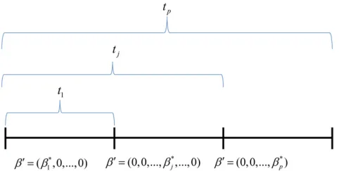
Figure 1 Example to illustrate why the pleiotropy LRT has an approxi-matex2
p21distribution when only onebjdiffers from zero. For this
ex-ample,b16¼0 andbj50ðj6¼iÞ:Then,t1will be the minimum because
it measures the sum of squared differences of thefitted values for the unconstrained ordinary least-squares model and the constrained model, which in this case is correctly specified. Because all othertjðj6¼1Þ
repre-sent misspecified models, their values can become arbitrarily large asn increases. Hence, the correctly specified model will have the smallest values oftj:And the distribution oftj for a correctly specified model is
x2
subsequent analyses (Vansteelandtet al.2009). Another ap-proach is based on Bayesian methods to partition associations into unassociated, indirect, and direct associations. However, it is difficult to accurately classify the type of causal associa-tion, particularly when residual correlations are large (e.g., it is difficult to discriminate between direct and indirect effects) (Stephens 2013).
The above methods are used to test whether a single genetic variant is associated with multiple traits. When scaling up to genome-wide data, it has been useful to use all the genetic markers to estimate the marker-predicted heritability of a trait. This has recently been extended to multiple traits to estimate pleiotropy as the genetic correlation of multiple traits. Mixed models are used to partition the phenotype correlations into genetic correlation (i.e., correlation of poly-genic total genetic values) and environmental correlation (Korte et al. 2012; Lee et al. 2012; Zhou and Stephens 2014; Furlotte and Eskin 2015). Although this approach does not evaluate whether particular SNPs or particular genomic regions are the cause for phenotype correlations, it has the potential to guide design of studies that focus on pleiotropy. For example, the correlation of two phenotypes can be par-titioned asrP5h1h2rg1e1e2re;whereh2i is the heritability of traiti,e2
i 512h2i;rgis the genetic correlation, andre is
the environmental correlation (Falconer and Mackay 1996, p. 314). Heritability in the narrow sense is the percentage of the variance of the trait explained by additive genetic fac-tors. This illustrates that if both traits have low heritability, the phenotype correlation is primarily due to environmental correlation (and nonadditive genetic effects that are missed byrg), implying that large sample sizes would be needed to
test pleiotropy when there are small genetic effects.
We have emphasized that current methods to evaluate pleiotropy do not perform a formal test of the null hypothesis of no pleiotropy. For the special case of two traits, one can construct a null hypothesis of no pleiotropy based on the intersection-union (IU) test (Silvapulle and Sen 2004). Consider the regression equation yj5bo;j1b1;jg1ej;whereyj is the
vector of values for thejth trait,bo;jis the intercept,b1;iis the slope association parameter of interest,gis the vector of doses for the minor allele, andejis a vector of residuals. The union
null hypothesis is H0:b1;1 50 or b1;250;and the
intersec-tion alternative hypothesis is H1:b1;16¼0 and b1;26¼0:
Test-ing eachb1;iat a desired type I error, saya50:05;the null is rejected only if both tests reject. There is no need to correct for multiple testing, because the type I error rate is not inflated by this procedure. But this approach can be conser-vative, particularly if the two tests are uncorrelated. The IU test can be extended top.2 traits, but rejection of the null would occur only when allptests are significant at the spec-ifieda:For our situation, we wish to reject the null if at least two of theptests reject. One approach would be to apply the IU test to each pair of traits and reject the null if at least one of the IU tests rejects. But this would entail many pairs of tests, and for this situation one would need to correct for testing multiple pairs. Bonferroni correction would lead to an overly conservative test.
Because of current limitations, we developed a likelihood-ratio test for testing the null hypothesis of no pleiotropy—the null hypothesis that one or no traits are associated with a genetic variant vs. the alternative hypothesis that two or more traits are associated. We then extended the testing framework to test the null hypothesis thatkor fewer traits are associatedvs.the alternative hypothesis that more thank Table 1 Empirical type I error rate for common correlation
structure when b151 and all other bj50 ðj6¼1Þ; based on multivariate normal distribution
Sample size No. traits
Trait correlation
Nominal type I error rate
0.05 0.01
100 4 0.2 0.072 0.020
0.5 0.070 0.016
0.8 0.066 0.014
10 0.2 0.105 0.036
0.5 0.092 0.032
0.8 0.094 0.029
500 4 0.2 0.056 0.017
0.5 0.058 0.011
0.8 0.058 0.009
10 0.2 0.061 0.010
0.5 0.056 0.011
0.8 0.068 0.019
1000 4 0.2 0.052 0.012
0.5 0.058 0.008
0.8 0.051 0.010
10 0.2 0.057 0.012
0.5 0.052 0.010
0.8 0.046 0.007
Underlined values are for when empirical type I error exceeds the upper 95% C.I.
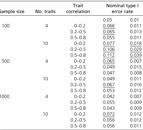
Table 2 Empirical type I error rate for random correlation structure when b151 and all other bj50 ðj6¼1Þ; based on multivariate normal distribution
Sample size No. traits
Trait correlation
Nominal type I error rate
0.05 0.01
100 4 0–0.2 0.066 0.011
0.2–0.5 0.065 0.013 0.5–0.8 0.055 0.011
10 0–0.2 0.077 0.018
0.2–0.5 0.106 0.029 0.5–0.8 0.112 0.039
500 4 0–0.2 0.065 0.007
0.2–0.5 0.049 0.015 0.5–0.8 0.047 0.008
10 0–0.2 0.049 0.011
0.2–0.5 0.067 0.016 0.5–0.8 0.053 0.012
1000 4 0–0.2 0.042 0.007
0.2–0.5 0.055 0.009 0.5–0.8 0.043 0.009
10 0–0.2 0.072 0.012
traits are associated (k50;1; :::p21). By this generaliza-tion, we propose sequential testing to test the null hypoth-esis that k11 traits are associated, given that the null hypothesis of ktraits are associated was rejected. This se-quential approach provides a refined approach to evaluate how many traits, and which traits, are associated with a genetic variant, accounting for correlation among the traits and possibly adjusting for covariates that could differ across the traits.
Methods
Likelihood-ratio test of pleiotropy: null of one or fewer traits
Suppose thatptraits are measured on each ofnsubjects. Let yj95ðyj1; :::;yjnÞdenote the vector of measures on thejth trait for nsubjects. Assume that each trait is modeled by linear regression, denoted
yj5xbj1ej;
where xis the dose of the minor allele fornsubjects. Also assume that allyj andxare centered, so intercepts can be
ignored. For simplicity of presentation, we ignore adjusting covariates, but our methods are general and allow for trait-specific covariates. By stacking vectors, we can express the model as y5Xb1e; where y9 5ðy19; :::;yp9Þ; X5diagðxÞ; b9 5ðb1; :::;9 b9pÞ; and e9 5ðe91; :::;e9pÞ: The error term
eNð0;VÞ;whereV5S5I;Iis ann3nidentity matrix, 5 is the Kronecker product, and thep3pmatrixS is the covariance matrix for the within-subject covariances of the errors. Under this model, the log-likelihood function ofðb;SÞ is given by
lnðb;SÞ5 2n
2logjSj2 1
2ðy2XbÞ9
S215Iðy2XbÞ:
Suppose that the covarianceSis known; otherwise, we can obtain a consistent estimate by maximum-likelihood estima-tion. For example, we can estimatebby using methods from seemingly unrelated regression, an approach called feasible generalized least squares. Separate ordinary linear regression for each trait can be used to obtain residuals to estimateSb;and then this is used in the generalized least-squares (GLS) solution,
b
b5hX9Sb215IXi21X9Sb215Iy:
Note that the feasible generalized least squares is asymptot-ically equivalent to maximum-likelihood estimation (MLE). There are two special cases when separate ordinary regres-sions and GLS result in the same solution: (1) when Sis a diagonal matrix and (2) when the regressors in Xj are the same for all traits. Hence, for the case where each trait is regressed on the samex, without additional adjusting cova-riates, separate ordinary least-squares regression and GLS give the same results. The covariance matrix of the residuals then provides a consistent estimate ofS:Then, the Cholesky decompositon ofVisV5V1=2V1=2;whereV1=25S1=25I and V21=25S21=25I: We then decorrelate the data by
~
y5V21=2y
and X~5V21=2X; to transform the model to
~
y5X~b1~e; where ~e5V21=2eNð0;InpÞ; which has log-likelihoodlnðbÞ5 2ð1=2Þð~y2X~bÞ9ð~y2X~bÞ:Based on this log likelihood, we derived the likelihood-ratio test (LRT) to test the null hypothesis of no pleiotropy: One or no traits are associated with a genetic variant. Below we outline how to compute the LRT and provide details of the deriva-tions inAppendix B.
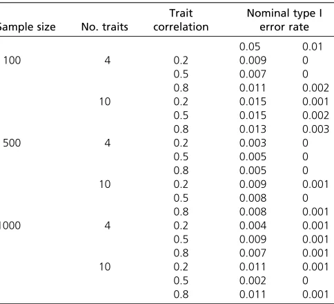
Table 3 Empirical type I error rate for common correlation structure when all bj50; based on multivariate normal distribution
Sample size No. traits
Trait correlation
Nominal type I error rate
0.05 0.01
100 4 0.2 0.005 0.002
0.5 0.006 0.001
0.8 0.009 0.002
10 0.2 0.015 0
0.5 0.011 0
0.8 0.014 0.003
500 4 0.2 0.003 0
0.5 0.005 0.001
0.8 0.011 0.001
10 0.2 0.005 0.001
0.5 0.003 0.001
0.8 0.009 0.001
1000 4 0.2 0.005 0
0.5 0.008 0
0.8 0.004 0.001
10 0.2 0.011 0.002
0.5 0.012 0
0.8 0.009 0.002
Table 4 Empirical type I error rate for random correlation structure when all bj50; based on multivariate normal distribution
Sample size No. traits
Trait correlation
Nominal type I error rate
0.05 0.01
100 4 0–0.2 0.005 0
0.2–0.5 0.012 0.001 0.5–0.8 0.014 0.001
10 0–0.2 0.018 0.002
0.2–0.5 0.01 0.002
0.5–0.8 0.029 0.004
500 4 0–0.2 0.004 0
0.2–0.5 0.009 0
0.5–0.8 0.007 0.001
10 0–0.2 0.009 0
0.2–0.5 0.009 0.001 0.5–0.8 0.019 0.005
1000 4 0–0.2 0.006 0.001
0.2–0.5 0.006 0
0.5–0.8 0.004 0
10 0–0.2 0.01 0.002
0.2–0.5 0.01 0
The null hypothesis of no pleiotropy can be expressed as
H0:Of the parameters b1;:::;bp; there exists at most one that is nonzero 4H1:otherwise:
The null hypothesis is equivalent to testing whether one of the followingp11 tests holds,
Hk0:bk6¼0;bj50ðj6¼kÞ;
for k50;. . .;p: Note that H00 represents all bk50 ðk51;. . .;pÞ; while fork.0;Hk0 allowsbk6¼0 while all otherbj50 ðj6¼kÞ:To represent thesep11 hypotheses, we use Hk0 :Vkb50: Let V0 be a matrix such that H00:V0b50 tests whether allbj50:This is the usual mul-tivariate test. In this case,V0is the identity matrix of dimen-sionp:To constructVk ðk.0Þ;create an identity matrix of
dimension p and then remove thekth row. This results in Vkb5ðb1; :::;bk21;bk11bpÞ9: Then, the null hypothesis is equivalent to
H0:There exists one of Hk0:Vkb50; for k50;. . .;p:
To construct the LRT, centeryandxabout their means, use ordinary least squares to estimate b; use the residuals to estimateS;and then useSto decorrelateyandXaccording to ~y5V21=2y; X~5V21=2X; where V21=25S21=25I: Then, for eachk50;. . .;p;compute
tk5y~9X~
~ X9X~21Vk
"
Vk
~ X9X~21Vk9
#21
Vk
~
X9X~21X~9~y:
An alternative way to expresstk istk5X~bn2X~bVk 2
;the squaredl2norm between thefitted values based on the
ordi-nary least-squares estimates,bn;and thefitted values based on the constrained estimates,bVk(seeAppendix B).
As shown inAppendix B, the LRT is
T5 min
k50;...;ptk:
Becausetjis based on the sum of squared differences of the fitted values between the unconstrained and constrained models, for a correctly specified constrained model,tjhas a
x2distribution. But the distribution ofTis more complicated.
The statistic T has two different asymptotic distributions depending on whenb¼0 or not. Whenb50;the asymp-totic distribution of eachtjis ax2distribution, yet the distri-bution of the minimum of them,T;is unknown. Alternatively, whenb50;we can use the commonly usedx2test for the
null hypothesis that allbj50:This motivates us to do the test by two stages. Thefirst stage is to just test H00:b50;using
the statistic t0x2p as the test statistic, so we reject H00 if
t0.x2pðaÞ;wherex2pðaÞis the 12aquantile of thex2 distri-bution withpd.f. If H00cannot be rejected, then the H0of no
pleiotropy cannot be rejected. If H00is rejected, we turn to the
second stage to test the null hypothesis that one Hk0holds for
k51;. . .;p:For this we ignoret0and use the test statistic
T15 min
k51;...;ptk:
SinceT1x2p21;we reject the null hypothesis that only one Hk0holds fork51;. . .;pifT1.x2p21ðaÞ:Then, the null
hy-pothesis H0 of no pleiotropy is rejected only if both H00 is
rejected and the null hypothesis that only one Hk0 holds is
rejectedðk51;. . .;pÞ:
To provide intuition whyT1 has a large samplex2
distri-bution with (p 2 1) d.f. when only one bj differs from zero, while all others equal zero, we present an example in
Table 5 Empirical type I error rate when b151and all other
bj50 ðj6¼1Þ; based on multivariate t distribution with 3 d.f., with common correlation structure
Sample size No. traits
Trait correlation
Nominal type I error rate
0.05 0.01
100 4 0.2 0.042 0.011
0.5 0.067 0.019
0.8 0.057 0.015
10 0.2 0.088 0.018
0.5 0.104 0.028
0.8 0.094 0.030
500 4 0.2 0.059 0.011
0.5 0.038 0.007
0.8 0.043 0.009
10 0.2 0.041 0.016
0.5 0.059 0.021
0.8 0.050 0.010
1000 4 0.2 0.052 0.006
0.5 0.047 0.006
0.8 0.054 0.009
10 0.2 0.054 0.010
0.5 0.058 0.015
0.8 0.055 0.016
Underlined values are for when empirical type I error exceeds the upper 95% C.I.
Table 6 Empirical type I error rate when all bj50; based on multivariatetdistribution with 3 d.f., with common correlation structure
Sample size No. traits
Trait correlation
Nominal type I error rate
0.05 0.01
100 4 0.2 0.009 0
0.5 0.007 0
0.8 0.011 0.002
10 0.2 0.015 0.001
0.5 0.015 0.002
0.8 0.013 0.003
500 4 0.2 0.003 0
0.5 0.005 0
0.8 0.005 0
10 0.2 0.009 0.001
0.5 0.008 0
0.8 0.008 0.001
1000 4 0.2 0.004 0.001
0.5 0.009 0.001
0.8 0.007 0.001
10 0.2 0.011 0.001
0.5 0.002 0
Figure 1. In this example b16¼0 and bj50 ðj6¼1Þ: As shown inAppendix B(Corollary 1), the distribution oftjfor a correctly specified model isx2
p21:In contrast, the incorrect models result in arbitrarily large values oftj(seeCorollary 2
inAppendix B). This means that t1 will be minimum and
T5t1 x2p21:
General likelihood-ratio sequential testing: null of K associated traits
The above sequential approach is based on testing the null hypothesis H00:b50;and then if this rejects, to turn to the
second stage to test the null hypothesis that only one Hk0:bk6¼0;bj50 ðj6¼kÞ holds for k51;. . .;p: The advantage of this approach is that if H00is rejected and the
null hypothesis that only one Hk0 holds is accepted, we can
conclude that there is only one nonzero b: But if the null hypothesis that only one Hk0 holds is rejected, we cannot
make afirm conclusion about the number of traits associated with a genetic variant. To provide a more rigorous testing framework, we extended our approach to sequentially test the null hypothesis that a specified number ofb’s are non-zero. So, if the null hypothesis that k b’s are nonzero is rejected, but the null hypothesis that k11b’s are nonzero is accepted, we can conclude there arek11 traits associated with a genetic variant. Furthermore, because the sequential testing is based on a likelihood-ratio framework, evaluating all possible combinations of nonzero b’s, the combination that fails to reject the null hypothesis provides evidence of which traits are associated with the genetic variant. The
de-tails of the statistical procedures of this general sequential testing method are provided inAppendix B, as well as a proof that the type I error is controlled. In summary, this general sequential procedure provides a formal way to determine not only they number of traits associated with a genetic variant, but also which traits are associated.
Simulations
To evaluate the adequacy of thex2distribution for the LRT,
we performed simulations. For the pleiotropy null, we per-formed two sets of simulations. Thefirst one assumed that all
bj50;the usual null for multivariate data. The second one fixedb1 51 and all otherbj50ðj52; :::;pÞ:The value of
b151 was chosen because the power for detecting this mar-ginal effect size was very large for our setup. We assumed three different sample sizes, n5100;500;1000;and two different values of p54;10: The small sample size of n5100 was used to evaluate the adequacy of our asymptotic derivations for small samples. The variance of the errors was assumed to be 1, and the covariance was assumed to be either a constantrfor all pairs of traits (i.e., exchangeable correla-tion structure) or a range of covariances. For the range of covariances, we randomly chose covariances from a specified range, assuming a uniform distribution of the covariances. With a specified covariance structure, we simulated the ran-dom errors from either a multivariate normal distribution or a multivariatetdistribution with 3 d.f., to evaluate the impact of heavy-tailed distributions. For all simulations, a single SNP was simulated, assuming a minor allele frequency of 0.2.
To evaluate the power of our proposed LRT for pleiotropy, we simulated 10 traits from a multivariate normal distribution with variances of 1 and equal covariances among the traits, set at r50:2;0:5;or0:8; for a total of n¼ 500 subjects. The number of traits associated with the SNP ranged over two, three, or five. The marginal effect of a trait was set at
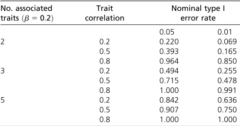
b50:25:This effect size explains 2% of the variation of a trait, and there is 90% power to detect a marginal effect of this size, using nominala50:05:We also set the marginal effect to
b50:2;which corresponds to an explained 1.2% of the varia-tion of a trait, and there is 70% power to detect a marginal effect of this size. All simulations were repeated 1000 times.
Data application
Our newly developed LRT for pleiotropy was applied to a data set that has 10 immunologic phenotypes measured in re-sponse to primary smallpox vaccination. These phenotypes included measures of humoral immunity (neutralizing anti-body titer) and cellular immunity [two separate IFNg ELISPOT assays and cytokine secretion upon viral stimulation as measured by ELISA (IL-1b, IL-2, IL-6, IL-12p40, IFNa, IFNg, TNFa)]. All 645 subjects included in the presented analyses were of Caucasian ancestry. All subjects provided informed consent for use of their samples and this study was approved by the Mayo Clinic Institutional Review Board. A genome-wide association of the 10 phenotypes was per-formed, with each phenotype adjusted for relevant covariates
(i.e.,P-value ,0.10 for association of a covariate with the phenotype, including eigenvectors to adjust for potential population stratification). Details of the study can be found in prior published reports (Kennedy et al. 2012a,b; Ovsyannikovaet al.2012a,b, 2013, 2014).
Data availability
Software implementing the proposed tests for pleiotropy for quantitative traits is available as an R package called“pleio”in the Comprehensive R Archive Network (https://cran.r-project. org/web/packages/pleio/index.html).
Results
Simulation results
The type I error rates based on simulations are presented in Table 1, Table 2, Table 3, Table 4, Table 5, and Table 6. For all simulations, we show results from the two-stage test (us-ingt0 for stage 1 andT15minftk;k51; :::;pgfor stage 2), but in all cases, the results from the two-stage test were identical to those from the compound pleiotropy test T5minftk;k50; :::;pg. The results for when only one bj differs from zero (Table 1, Table 2, and Table 5) illustrate that the LRT can have inflated type I error rates for small sample sizesðn5100Þ;with more extreme inflation asp in-creased from 4 to 10. In contrast, for moderate to large sam-ple sizesðn5500;1000Þ;the type I error rates were close to the nominal level, with only an occasional slight inflation. The inflated type I error rate for small sample sizes seems to be caused by the need to estimate the covariance matrix of the residuals. When we simulated errors that were in-dependent and used the identity matrix for the residual correlations, the simulated type I error rates were very close to the nominal rates for all sample sizes. In contrast, when allbjwere zero (Table 3, Table 4, and Table 6), the LRT has conservative type I error rates. This, however, is not of con-cern, because controlling the type I error rate when only onebjdiffers from zero is the major error that should be con-trolled when testing pleiotropy. These results were consistent
for different amounts and patterns of residual correlations and for multivariate normal and multivariatetdistributions.
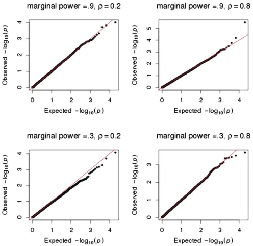
To further evaluate the adequacy of our asymptotic ap-proximations for large samples, we performed 10,000 simu-lations for 1000 subjects and four traits that had a common correlation structure. All but one b was zero; the nonzero
bwas chosen such that there was either 90% or 30% power to detect its marginal effect using a50:001: This scenario reflects modern large-scale genomic studies that use more stringent significance thresholds. The quantile–quantile plots in Figure 2 show that the asymptotic x2 distribution to test
pleiotropy provides adequateP-values over the entire range of P-values for when the marginal effect of onebis small (power of 30%) or large (power of 90%) and for when the correlation of the traits is smallðr50:2Þor largeðr50:8Þ:
The simulation-based power is illustrated in Table 7 and Table 8. The general patterns show that the power to detect two or more associated traits increases with the number of truly associated traits, the effect size of each trait, and larger residual correlations among the traits.
To provide insights into the properties of our proposed sequential testing of multiple traits, we simulated six traits with a common correlation structure such that three of the traits were associated with a genetic variant (i.e., three true nonzero b’s). The effect sizes of the associated traits were chosen to have marginal power of 0.3, 0.7, or 0.9 for a sample size of 1000 subjects. These marginal effect sizes correspond to 0.2%, 0.6%, and 1.0% explained variation of the marginal trait. A total of 1000 simulations were performed. The results are presented in Table 9. The frequency of accepting the null hypothesis that allb’s¼0 (e.g., nob’s selected to be associ-ated with the genetic variant) ranged from 0.646 for when power was 0.3 to 0.015 when power was 0.9—not surprising that greater power resulted in greater frequency of selecting at least one bto be nonzero. Table 9 also presents the fre-quency for which the three true nonzerob’s were selected, conditional on at least one of the six b’s was selected. For weak marginal power (e.g., power of 0.3), the frequency of selecting all three nonzero b’s was small (0.034–0.213,
Table 8 Power to detect pleiotropy when associated traits have b50:2(explain 1.2% trait variation; power570% for marginal effect)
No. associated traitsðb50:2Þ
Trait correlation
Nominal type I error rate
0.05 0.01
2 0.2 0.220 0.069
0.5 0.393 0.165
0.8 0.964 0.850
3 0.2 0.494 0.255
0.5 0.715 0.478
0.8 1.000 0.991
5 0.2 0.842 0.636
0.5 0.907 0.750
0.8 1.000 1.000
Shown is a multivariate normal distribution with equal correlation structure, for a sample size of 500 subjects and minor allele frequency of genetic variant set to 0.20.
Table 7 Power to detect pleiotropy when associated traits have b50:25(explain 2% trait variation; power590% for marginal effect)
No. associated traitsðb50:25Þ
Trait correlation
Nominal type I error rate
0.05 0.01
2 0.2 0.503 0.237
0.5 0.801 0.581
0.8 0.971 0.900
3 0.2 0.859 0.677
0.5 0.956 0.858
0.8 0.999 0.998
5 0.2 0.980 0.928
0.5 0.999 0.985
0.8 1.000 1.000
depending on the trait correlation). Yet the frequency of selecting at least one of the three nonzerob’s was reasonable (0.747–0.862). The frequency of correctly selecting all three nonzerob’s increased as either marginal power increased or trait correlation increased. For example, for marginal power of 0.7, the frequency of selecting all three nonzerob’s was 0.179 for weak correlation (r ¼ 0.2), and was 0.851 for strong correlation (r¼0.8). For marginal power of 0.9, the frequency of selecting all three nonzero b’s was 0.472 for weak correlation (r¼0.2), and was 0.956 for strong correla-tion (r¼0.8). In contrast to selecting true nonzerob’s, we also present in Table 9 the frequency of wrongly selectingb’s that are truly zero. Not surprisingly, when marginal power is weak (power of 0.3), if at least onebis selected, there is a significant chance of wrongly selecting a true-zerob(e.g., frequency of 0.209 when r ¼ 0.2). This type of error decreased as the marginal power for traits increased and the trait correlation increased. For example, when power was 0.9 and trait corre-lation wasr¼0.8, the frequency of selecting one true-zerob was 0.034, approaching the nominal type I error rate of 0.05. Table 9 illustrates that although there is a chance of wrongly selecting one true-zerob;the frequency of selecting more than one true-zerobwas small.
Data application results
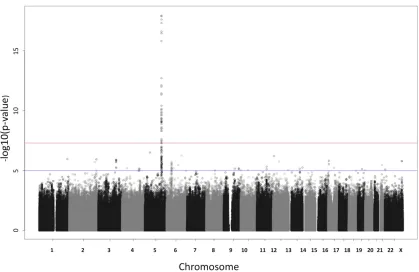
Based on the traditional multivariate regression of all 10 traits on each SNP, we found a strong association of at least one of the traits with SNPs in a region on chromosome 5 (see Figure 3). Figure 4 illustrates the traditional multivariate testðt0Þin
a small region of chromosome 5 (left panel) and the LRT of pleiotropy in the same region (right panel). The test for plei-otropy provides strong evidence that the signal of association was driven by a single phenotype. This is confirmed qualita-tively in Figure 5, which shows the individual marginal trait associations for the chromosome 5 region. Although the in-dividual marginal associations in Figure 5 give the visual impression that only one trait is strongly associated with the chromosome 5 SNPs, the LRT of pleiotropy provides a formal statistical test that accounts for the correlations among the traits.
Discussion
Genetic pleiotropy has been of scientific interest since the time of Gregor Mendel, as he described different traits in peas controlled by genes, such as pea coat color and texture, color of
flowers, and whether there were axial spots. In current re-search, understanding pleiotropy can aid the understanding of complex biological mechanisms of genes (as shown in our vaccine response data), as well as aid the development of pharmacologic and vaccine targets. Yet the statistical methods to assess pleiotropy have resorted to ad hoccomparison of univariate statistical tests or multivariate methods that test the null hypothesis of no trait associations. Because a formal statistical test of pleiotropy was lacking, we developed a novel LRT statistic. The statistic is easy to compute, based
on well-known linear regression methods for quantitative traits. Our simulations show that the LRT closely follows a
x2distribution when only one trait is associated with a
ge-netic variant and that the LRT tends to be conservative when no traits are associated. We proposed a sequential testing procedure, where the null hypothesis of no associ-ated traits could be testedfirst (using standard multivariate regression methods) and, if significant, be followed by a test of whether only one trait is associated. If the test of only one associated trait rejects, we proposed sequential testing the null ofjassociated traits (j¼2,. . .,p21), until the sequential test fails to reject the null hypothesis. This approach provides a way to assess the number of traits associated with a genetic variant, accounting for the corre-lations among the traits. A limitation of our approach, and most other methods for associations of genetic variants with multiple traits, is that it has limited power when an allele is rare. An alternative approach is to compare the similarity of multiple traits with the similarity of rare-variant genotypes across a genetic region, for pairs of subjects (Broadaway
et al.2016). The benefit of this approach is balanced with
the limitation of not knowing which genotypes are associ-ated with which traits. Our proposed sequential testing might provide a worthy follow-up procedure if some vari-ants are not too rare.
Although our proposed methods assumed the subjects are independent, it is straightforward to extend our approach to pedigree data. To do so, the variance matrix of residuals for independent subjects,VðeÞ5ðS5IÞ;would be replaced with VðeÞ5ðS5KÞ: The matrix K contains diagonal elements
Kii511hi;wherehiis the inbreeding coefficient for subject i, and off-diagonal elementsKij52uij:The parameteruij is the kinship coefficient between individualsiandj, the prob-ability that a randomly chosen allele at a given locus from individualiis identical by descent to a randomly chosen allele from individualj, conditional on their ancestral relationship. For subjects from different pedigrees, uij 50;so K can be structured as a block-diagonal matrix, with diagonal block Ki for theith pedigree. With this adjustment, our methods
can be used for pedigree data or for data with population structure where matrixKis an estimate of genetic relation-ships (Schaidet al.2013).
Application of our new approach to a study of immune phenotypes in response to smallpox vaccination strongly
Figure 3 Manhattan plot of the multivariate regression of 10 traits on each SNP, using statistict0;to test whether any of the traits are associated with
an SNP. The upper red horizontal line corresponds to aP-value of 531028and the lower blue line to aP-value of 1025:
suggests that only 1 of 10 correlated traits is statistically associated with SNPs in a region on chromosome 5. The benefit of this type of analysis is that it provides strong guidance on follow-up functional studies for genome-wide association studies with multiple traits. In our case, it allowed investigators to focus on the single immunologic trait truly associated with the chromosome 5 SNPs, rather than con-ducting labor-intensive, expensive, and time-consuming ex-periments on unrelated immune response traits.
We recognize that our proposed LRT depends on the assumption that residuals have a multivariate normal distri-bution. Our simulations with a multivariate t distribution (3 d.f.) suggest that the LRT is robust to heavy-tailed distri-butions. To ensure robustness with the traditional multivar-iate regression, it is common practice to transform the data to have at least normally distributed marginal distributions, such as use of normal quantile transformation. This is a rea-sonable approach for our proposed LRT.
A limitation of our method is that each of the traits is assumed to be quantitative. If all traits are binary, or if there is a mixture of quantitative and binary traits, then the dependence of the LRT on an assumed likelihood would need to be reconsidered. One approach is to consider a general multi-variate exponential family of models (Prentice and Zhao 1991; Zhao et al. 1992; Sammelet al.1997). Another ap-proach would be to consider the reverse regression of an SNP dose on all traits, like the ordinal logistic MultiPhen approach of O’Reilly et al. (2012), yet develop an LRT for
pleiotropy whereby one of the b’s is allowed to be uncon-strained under the null. An alternative approach that we are developing is based on generalized linear models and generalized estimating equations. The theoretical underpin-nings of these alternate approaches, and their computational challenges, are topics of future research.
Acknowledgments
This research was supported by (1) the U.S. Public Health Service, National Institutes of Health (NIH), grant GM065450 (to D.J.S.); (2) federal funds from the National Institute of Allergies and Infectious Diseases, NIH, Depart-ment of Health and Human Services, under contract HHSN266200400025C (N01AI40065) (to G.A.P.); and (3) the National Natural Science Foundation of China (grant 11371062), Beijing Center for Mathematics and Information Interdisciplinary Sciences, China Zhongdian Project (grant 11131002) (to X.T.). The content is solely the responsibility of the authors and does not necessarily represent the official views of the NIH. G.A.P. is the chair of a Safety Evaluation Committee for novel investigational vaccine trials being conducted by Merck Research Laboratories. G.A.P. offers consultative advice on vaccine development to Merck & Co. Inc., CSL Biotherapies, Avianax, Dynavax, Novartis Vaccines and Therapeutics, Emergent Biosolutions, Adjuvance, and Microdermis. G.A.P. holds two patents related to vaccinia and measles peptide research. R.B.K. has grant funding from
Merck Research Laboratories to study immune responses to mumps vaccine. These activities have been reviewed by the Mayo Clinic Conflict of Interest Review Board and are con-ducted in compliance with Mayo Clinic Conflict of Interest policies. This research has been reviewed by the Mayo Clinic Conflict of Interest Review Board and was conducted in compliance with Mayo Clinic Conflict of Interest policies.
Literature Cited
Berkson, J., 1946 Limitations of the application of fourfold table analysis to hospital data. Biom. Bull. 2(3): 47–53.
Broadaway, K. A., D. J. Cutler, R. Duncan, J. L. Moore, E. B. Wareet al., 2016 A statistical approach for testing cross-phenotype effects of rare variants. Am. J. Hum. Genet. 98(3): 525–540.
Cotsapas, C., B. F. Voight, E. Rossin, K. Lage, B. M. Neale et al., 2011 Pervasive sharing of genetic effects in autoimmune dis-ease. PLoS Genet. 7(8): e1002254.
Denny, J. C., L. Bastarache, M. D. Ritchie, R. J. Carroll, R. Zinket al., 2013 Systematic comparison of phenome-wide association study of electronic medical record data and genome-wide asso-ciation study data. Nat. Biotechnol. 31(12): 1102–1110. Falconer, D., and T. Mackay, 1996 Introduction to Quantitative
Genetics. Pearson Prentice Hall, New York.
Ferreira, M. A., and S. M. Purcell, 2009 A multivariate test of association. Bioinformatics 25(1): 132–133.
Furlotte, N., and E. Eskin, 2015 Efficient multiple-trait association and estimation of genetic correlation using the matrix-variate linear mixed model. Genetics 200: 59–68.
Galesloot, T. E., K. van Steen, L. A. Kiemeney, L. L. Janss, and S. H. Vermeulen, 2014 A comparison of multivariate genome-wide association methods. PLoS One 9(4): e95923.
Gianola, D., G. de los Campos, M. H. N. Toro, C. Schon, and D. Sorensen, 2015 Do molecular markers inform about pleiot-ropy? Genetics 201: 23–29.
Kennedy, R. B., I. G. Ovsyannikova, V. S. Pankratz, I. H. Haralambieva, R. A. Vierkantet al., 2012a Genome-wide genetic associations with IFNgamma response to smallpox vaccine. Hum. Genet. 131 (9): 1433–1451.
Kennedy, R. B., I. G. Ovsyannikova, V. S. Pankratz, I. H. Haralambieva, R. A. Vierkantet al., 2012b Genome-wide analysis of polymor-phisms associated with cytokine responses in smallpox vaccine re-cipients. Hum. Genet. 131(9): 1403–1421.
Korte, A., B. J. Vilhjalmsson, V. Segura, A. Platt, Q. Longet al., 2012 A mixed-model approach for genome-wide association studies of corre-lated traits in structured populations. Nat. Genet. 44(9): 1066–1071. Lee, S., J. Yang, M. Goddard, P. Visscher, and N. Wray, 2012 Estimation of pleiotropy between complex diseases using single-nucleotide polymorphism-derived genomic relationships and restricted max-imum likelihood. Bioinformatics 28: 2540–2542.
Liu, J., Y. Pei, C. J. Papasian, and H. W. Deng, 2009 Bivariate association analyses for the mixture of continuous and binary traits with the use of extended generalized estimating equa-tions. Genet. Epidemiol. 33(3): 217–227.
Maier, R., G. Moser, G. B. Chen, S. Ripke, W. Coryell et al., 2015 Joint analysis of psychiatric disorders increases accuracy of risk prediction for schizophrenia, bipolar disorder, and major depressive disorder. Am. J. Hum. Genet. 96(2): 283–294. Maity, A., P. F. Sullivan, and J. Y. Tzeng, 2012 Multivariate
phe-notype association analysis by marker-set kernel machine re-gression. Genet. Epidemiol. 36(7): 686–695.
Marchini, J., B. Howie, S. Myers, G. McVean, and P. Donnelly, 2007 A new multipoint method for genome-wide association studies by imputation of genotypes. Nat. Genet. 39(7): 906–913.
O’Reilly, P. F., C. J. Hoggart, Y. Pomyen, F. C. Calboli, P. Elliott
et al., 2012 MultiPhen: joint model of multiple phenotypes can
increase discovery in GWAS. PLoS One 7(5): e34861.
Ovsyannikova, I. G., I. H. Haralambieva, R. B. Kennedy, V. S. Pankratz, R. A. Vierkant et al., 2012a Impact of cytokine and cytokine receptor gene polymorphisms on cellular immu-nity after smallpox vaccination. Gene 510(1): 59–65. Ovsyannikova, I. G., R. B. Kennedy, M. O’Byrne, R. M. Jacobson, V. S.
Pankratzet al., 2012b Genome-wide association study of anti-body response to smallpox vaccine. Vaccine 30(28): 4182–4189. Ovsyannikova, I. G., I. H. Haralambieva, R. B. Kennedy, M. M. O’Byrne, V. S. Pankratz et al., 2013 Genetic variation in IL18R1 and IL18 genes and Interferon gamma ELISPOT re-sponse to smallpox vaccination: an unexpected relationship. J. Infect. Dis. 208(9): 1422–1430.
Ovsyannikova, I. G., V. S. Pankratz, H. M. Salk, R. B. Kennedy, and G. A. Poland, 2014 HLA alleles associated with the adaptive immune response to smallpox vaccine: a replication study. Hum. Genet. 133(9): 1083–1092.
Prentice, R. L., and L. P. Zhao, 1991 Estimating equations for parameters in means and covariances of multivariate discrete and continuous responses. Biometrics 47: 825–839.
Roy, J., X. Lin, and L. M. Ryan, 2003 Scaled marginal models for multiple continuous outcomes. Biostatistics 4(3): 371–383. Sammel, M., L. Ryan, and J. Legler, 1997 Latent variable models
for mixed discrete and continuous outcomes. J. R. Stat. Soc. B 59 (3): 667–678.
Schaid, D. J., S. K. McDonnell, J. P. Sinnwell, and S. N. Thibodeau, 2013 Multiple genetic variant association testing by collapsing and kernel methods with pedigree or population structured data. Genet. Epidemiol. 37(5): 409–418.
Schifano, E. D., L. Li, D. C. Christiani, and X. Lin, 2013 Genome-wide association analysis for multiple continuous secondary phenotypes. Am. J. Hum. Genet. 92(5): 744–759.
Schriner, D., 2012 Moving toward system genetics through multiple trait analysis in genome-wide association studies. Front. Genet. 16(7): 1–7. Silvapulle, M. J., and P. K. Sen, 2004 Constrained Statistical
In-ference: Order,Inequality,and Shape Constraints. John Wiley &
Sons, New York.
Solovieff, N., C. Cotsapas, P. H. Lee, S. M. Purcell, and J. W. Smoller, 2013 Pleiotropy in complex traits: challenges and strategies. Nat. Rev. Genet. 14(7): 483–495.
Stephens, M., 2013 A unified framework for association analysis with multiple related phenotypes. PLoS One 8(7): e65245. Vansteelandt, S., S. Goetgeluk, S. Lutz, I. Waldman, H. Lyonet al.,
2009 On the adjustment for covariates in genetic association analysis: a novel, simple principle to infer direct causal effects. Genet. Epidemiol. 33(5): 394–405.
Wu, M. C., P. Kraft, M. P. Epstein, D. M. Taylor, S. J. Chanocket al., 2010 Powerful SNP-set analysis for case-control genome-wide association studies. Am. J. Hum. Genet. 86(6): 929–942. Xu, Z., and W. Pan, 2015 Approximate score-based testing with
application to multivariate trait association analysis. Genet. Epi-demiol. 39(6): 469–479.
Yang, Q., and Y. Wang, 2012 Methods for analyzing multivariate phe-notypes in genetic association studies. J. Probab. Stat. 2012: 652569. Zhang, Y., Z. Xu, X. Shen, and W. Pan, 2014 Testing for association with multiple traits in generalized estimation equations, with ap-plication to neuroimaging data. Neuroimage 96: 309–325. Zhao, L. P., R. L. Prentice, and S. G. Self, 1992 Multivariate mean
parameter estimation by using a partly exponential model. J. R. Stat. Soc. B 54(3): 805–811.
Zhou, X., and M. Stephens, 2014 Efficient multivariate linear mixed model algorithms for genome-wide association studies. Nat. Methods 11(4): 407–409.
Appendices
Appendix A
R code to computeF-statistic for canonical correlation of matrixYwith vectorx. library(CCA)
cc.fit,- cc(Y,x)
cc.fstat,- function(cc.fit){ rho,- cc.fit$cor
lambda,- 1 - rho^2
dimx,- max(dim(cc.fit$xcoef)) dimy,- max(dim(cc.fit$ycoef)) k,- max(c(dimx, dimy)) n,- nrow(Y)
fstat,- ((1-lambda)/lambda) * ((n-k-1)/k) pval,- 1-pf(fstat, k, n-k-1, ncp¼0)
return(list(fstat¼fstat, pval¼pval)) }
Appendix B: Hypothesis Tests for Linear Model
Notation and model
Based on the regression model described in the main text, suppose thatptraits are measured on each ofnsubjects, with yj95ðyj1; :::;yjnÞthe vector of measures on thejth trait fornsubjects, and stack the vectors asy9 5ðy19; :::;yp9Þ:LetX5diagðxÞ;
wherexis a vector of lengthn. We assume thatyandxare centered on their means. We can express the model asy5Xb1e; wheree9 5ðe91; :::;e9pÞ:The error termeNð0;VÞ;whereV5S5Iand thep3pmatrixSis the covariance matrix for the
within-subject covariances of the errors. Then, the Cholesky decompositon of Vis V5V1=2V1=2;where V1=25S1=25I andV21=25S21=25I:Using~y5V21=2y; X~5V21=2X;the model can transform to independent standard normal random variables,~y5X~b1~e;where~e5S21=2eNð0;InpÞ;and with log likelihoodlnðbÞ5 2ð1=2Þðy~2X~bÞ9ð~y2X~bÞ:
Theorem 1.Let V be a k3p matrix of rank kðk#pÞ:Then the minimizer ofy~2X~b2under the constraintVb50is
bV5bn2b*V;
wherebn5ðX~9X~Þ2
1X~
9~yis the ordinary least-squares(OLS)estimate and
b*
V5
~ X9X~21V9
"
VX~9X~21V9 #21
VX~9X~21X~9~y:
Furthermore,
~y2X~bV25y~2X~bn21X~b* V
2
: (B1)
Proof. Denoteb*5bn2b:Note that
~y2X~b25 ~y2X~bn1X~ðbn2bÞ25ky~2Xbnk21b9
*X~9X~b *1 2~y2X~bn9X~b *5~y2X~bn21b9 *X~9X~b *:
The last above step results from 2ð~y2X~bnÞ9X~b*50;because~yX~ 5bn9X~9X~:
Under the constraintVb50;Vb*5Vbn:Applying the Lagrange multiplier method, we minimize
Qb*;l5y~2X~bn21b*X~9X~b*1 2lVb*2Vbn:
By taking the derivative ofQwith respect tobandl;we obtain the solutionb*
V 5ðX~9X~Þ21V9½VðX~9X~Þ21V921VðX~9X~Þ21X~9~yand
the estimate ofbisbV5bn2b* V:
~y2X~bV25~y2X~bn21b*
V9X~9X~b*V:
This completes theProof.
Remark. Equation B1 illustrates that the residual sums of squares (ssq) for the constrained model ~y2X~bV2
are partitioned into two parts: (1) the ssq for the OLSfit~y2X~bn2and (2) the sum of squared differences of thefitted values
for the OLS model and the constrained modelX~b* V
2
5X~bn2X~bV 2
:
Corollary 1.Under the null hypothesis,Vb50; X~b*
V 2
5 "
VX~9X~21V9
#21
V
~
X9X~21X~9~e
2
x2
k:
Proof.
X~b* V
2
5X~X~9X~21V9 "
VX~9X~21V9 #21
VX~9X~21X~9~y
2
5y~9X~X~9X~21V9½VX~9X~21V921VX~9X~21X~9X~
3X~9X~21V9½VX~9X~21V921VX~9X~21X~9y~
5y~9X~X~9X~21V9 "
VX~9X~21V9 #21
VX~9X~21X~9~y
5e9~X~X~9X~21V9½VX~9X~21V921VX~9X~21X~9~e:
The substitution of~ywith~ein the last step of the aboveProofcan be made because by the assumed linear model,y~5X~b1~e;we
find that
VX~9X~21X~9~y5VX~9X~21X~9X~b1~e5Vb1VX~9X~21X~9~e5VX~9X~21X~9~e:
The last step above results becauseVb50 under the null hypothesis.
It is easy to verify that the matrixPV 5X~ðX~9X~Þ21V9½VðX~9X~Þ21V921VðX~9X~Þ21X~9is idempotent and is of rankkif the rank ofV
is of rankk:Because~e5Nð0;InpÞandPVis idempotent,e9~PV~ex2k;completing theProof.
Corollary 2.IfVb06¼0;then
X~b* V
2
5OðnÞ/N:
Proof. It follows from theProofofCorollary 1thatX~b*
V 2
5y~9PV~y:By the linear model, we have
X~b*
V5y~9PVy~5b90X~9PVX~b01e9PVe12b90X~9PVe:
It is clear that e9PVex2k5Opð1Þ and b90X~9PVe5Opðn
1=2Þ: In addition, b9
0X~9PVX~b05ðVb0Þ9½VðX~9X~Þ21V921Vb5
nðVb0Þ9½Vðn21X~9X~Þ21V921Vb5
OðnÞsinceVðn21X~9X~Þ21V9/Vð
EX~9X~Þ21V9 5Oð1Þin probability. Combining all three facts yieldsCorollary 2.
Hypothesis tests
Now we consider the null hypothesis of no pleiotropy:
H0:Of the parameters b1;:::;bp;there exists at most one that is nonzero4H1:otherwise:
Hk0 :bk6¼0;bj50 ðj6¼kÞ;
for k50;. . .;p: Note that H00 represents all bk50 ðk51;. . .;pÞ; while for k.0; Hk0 allows bk6¼0 while all other
bj50 ðj6¼kÞ:
To represent thesep11 hypotheses, we use Hk0:Vkb50:LetV0be a matrix such that H00:V0b50 tests whether all
bj50:In this case,V0is the identity matrix of dimensionp:To constructVkðk.0Þ;create an identity matrix of dimensionp and then remove thekth row. This results inVkb5ðb1; :::;bk21;bk11bpÞ9:Then, the null hypothesis is equivalent to
H0:there exists one of Hk0:Vkb50; for k50;. . .;p :
Fork50;1;. . .;p;settk5y~9PVk~y:Then it follows fromTheorem 1that
tk5X~bVk
2
2X~bn2;
wherebVkis the least-squares estimate under the constraintVkb50 and
PVk5X~
~ X9X~21Vk9
"
Vk
~ X9X~21Vk9
#21
Vk
~
X9X~21X~9:
Then we have the following corollary.
Corollary 3.The LRT,223log of ratio of likelihoods,is given by
T5 min
k50;...;ptk:
If H00holds, then
tk5e9PVke;
andt0x2p; tkx2p21fork51;. . .;p:
If only one Hk0ðk.0Þholds, then
T x2p21:
FromCorollary 3, we can see that the test statisticThas two different asymptotic distributions whenb¼0 or not. Whenb50;the
asymptotic distribution ofTis unknown. Alternatively, whenb50;we can use the commonly usedx2
ptest for the null hypothesis that allbj50:This motivates us to do the test by two stages. Thefirst stage is just test H00 :b50;using the statistict0x2pas the test statistic, so we reject H00ift0.x2pðaÞ;wherex2pðaÞis the 12aquantile of ax2distribution withpd.f. If H00cannot be rejected,
then H0 cannot be rejected. If H00 is rejected, we turn to the second stage to test the null hypothesis that one Hk0 holds for
k51;. . .;p:Then we can use the test statisticT1 5mink51;...;ptk:SinceT1x2p21;we reject the null hypothesis that one Hk0holds
fork51;. . .;pifT1.x2p21ðaÞ:Then, the null hypothesis H0is rejected only if both H00is rejected and the null hypothesis that one
Hk0holds is rejectedðk51;. . .;pÞ:Since both tests are conducted at type I error rate ofa;and this is based on the principal of the IU
test (Silvapulle and Sen 2004), the type I error rate for rejecting H0 is no more thana:
Remark.Ifpis too large, it might be beneficial to ignore thet0and directly useT1x2p21to construct the rejection region.
Sequential test of nonzero betas
The above solutions can be easily extended to test the following null hypothesis:
H0:There exist at most K nonzero components of b 4H1:otherwise :
T5 min
k51;...;CKpkPVk~yk
2;
wherePVk5X~ðX~9X~Þ21Vk9½VkðX~9X~Þ21V92 1
k VkðX~9X~Þ21X~9:
In the above,Vkis aðp2KÞ3pmatrix. For example, if for indexes 1#i1,⋯,iK#p;we test
bi16¼0;. . .;biK 6¼ 0 and bj50;j6¼ i1;. . .;iK;
then we can constitute the corresponding matrixVi1;...;iKas follows: (i) Constitute ap3pidentity matrix and (ii) delete the rows for indexesi1;. . .;iK:
Then we can use the following multistage test:
i. First test H00:b50:Reject ift0.x2pðaÞ:If reject, go to the next stage; otherwise stop and conclude H00is true.
ii. For s51;. . .;K21; test Hs0 : there are only s components of b 6¼ 0. Reject Hs0 if Ts.x2p2sðaÞ; where Ts5min1#i1,⋯,is#py~9PVi1;...;is~y: The indexes range over the Csp choices. If reject, continue testing by incrementing s by 1. If fail to reject Hs0;stop testing and conclude there arestraits associated withx.
The type I error rate of this sequential testing is no greater than the nominalalevel. To understand this, suppose there areK nonzerob’s, and define the type I error as concluding there are. Knonzerob’s. Note that the test statisticTsat each stage is based on the minimum of statistics, where each statistic is based onX~b*
V 2
5X~bn2X~bV 2
;a measure of distance between
fitted values based on the unconstrained OLS model and the constrained model determined byV. If one of the constrained models is correct, then byCorollaries 1and2,Tsx2:If, however, none of the constrained models are correct,Ts5OðnÞ/N: This means that at testing stagej,K;the probability of rejecting the null hypothesis at stagejdepends on the power to detect the misspecified models, which approach 1 asnincreases. With this background, we can formally evaluate the type I error rate. Definerjas an indicator of whether the null hypothesis is rejected at stagej. The probability of a type I error is the probability of rejecting the sequential stage testing up to and including stageK. This joint probability can be expressed as
Pðr0;r1;r2; :::;rKÞ5Pðr0ÞPðr1jr0ÞPðr2jr0;r1Þ::PðrKjr0;r1; :::;rK21Þ: (B2)
The last term in expression (B2) represents the probability of rejecting the null hypothesis when the null hypothesis is true, so one of the constrained models is correct. The test statistic at stageKfollows ax2
p2Kdistribution, soPðrKjr0;r1; :::;rK21Þ5a:All