| INVESTIGATION
C
LEAR
: Composition of Likelihoods for Evolve and
Resequence Experiments
Arya Iranmehr,*,1Ali Akbari,* Christian Schlötterer,†and Vineet Bafna‡
*Department of Electrical and Computer Engineering, and‡Department of Computer Science and Engineering, University of California, San Diego, California 92093, and†Institut für Populationsgenetik, Veterinärmedizinische Universität Wien, 1210 Vienna, Austria ORCID IDs: 0000-0002-8404-9797 (A.I.); 0000-0002-5000-5876 (A.A.); 0000-0003-4710-6526 (C.S.)
ABSTRACT The advent of next generation sequencing technologies has made whole-genome and whole-population sampling possible, even for eukaryotes with large genomes. With this development, experimental evolution studies can be designed to observe molecular evolution“in action”via evolve-and-resequence (E&R) experiments. Among other applications, E&R studies can be used to locate the genes and variants responsible for genetic adaptation. Most existing literature on time-series data analysis often assumes large population size, accurate allele frequency estimates, or wide time spans. These assumptions do not hold in many E&R studies. In this article, we propose a method—composition of likelihoods for evolve-and-resequence experiments (CLEAR)—to identify signatures of selection in small population E&R experiments. CLEARtakes whole-genome sequences of pools of individuals as input, and properly addresses heterogeneous ascertainment bias resulting from uneven coverage. CLEAR also provides unbiased estimates of model parameters, including population size, selection strength, and dominance, while being computationally efficient. Extensive simulations show that CLEARachieves higher power in detecting and localizing selection over a wide range of parameters, and is robust to variation of coverage. We applied the CLEARstatistic to multiple E&R experiments, including data from a study of adaptation ofDrosophila melanogasterto alternating temperatures and a study of outcrossing yeast populations, and identified multiple regions under selection with genome-wide significance.
KEYWORDSexperimental evolution; selection; genetic drift; time-series data; hidden Markov model; Wright–Fisher process
N
ATURAL selection is a key force in evolution, and a mechanism by which populations can adapt to external“selection”pressure. Examples of adaptation abound in the natural world (Fan et al.2016), including classic examples like lactose tolerance in Northern Europeans (Bersaglieri et al.2004), human adaptation to high altitudes (Simonson et al.2010; Yiet al.2010), but also drug resistance in pests (Daborn et al. 2001), HIV (Feder et al. 2016), cancer (Gottesman 2002; Zahreddine and Borden 2013), malarial parasite (Nair et al. 2007; Ariey et al. 2014), and others
(Spellberg et al. 2008). In these examples, understanding the genetic basis of adaptation can provide valuable informa-tion, underscoring the importance of the problem.
Experimental evolution refers to the study of the evolution-ary processes of a model organism in a controlled (Hegreness et al. 2006; Bollback and Huelsenbeck 2007; Barrick et al. 2009; Langet al.2011; Orozco-ter Wengelet al.2012; Lang et al.2013; Ozet al.2014) or natural (Barrettet al.2008; Reid et al. 2011; Denef and Banfield 2012; Winterset al. 2012; Daniels et al. 2013; Maldarelliet al. 2013; Bergland et al. 2014) environment. Recent advances in whole-genome se-quencing have enabled us to sequence populations at a reason-able cost, even for large genomes. Perhaps more important for experimental evolution studies, we can now evolve and rese-quence (E&R) multiple replicates of a population to obtain longitudinal time-series data, to investigate the dynamics of evolution at the molecular level. Although constraints such as small sizes, limited timescales, and oversimplified labora-tory environments may limit the interpretation of E&R results, Copyright © 2017 by the Genetics Society of America
doi:https://doi.org/10.1534/genetics.116.197566
Manuscript received November 3, 2016; accepted for publication March 31, 2017; published Early Online April 6, 2017.
Available freely online through the author-supported open access option.
Supplemental material is available online atwww.genetics.org/lookup/suppl/doi:10. 1534/genetics.116.197566/-/DC1.
1Corresponding author: EBU3 Room 4250, Department of Electrical and Computer
these studies are increasingly being used to test a wide range of hypotheses (Kaweckiet al.2012) and have been shown to be more predictive than static data analysis (Sawyer and Hartl 1992; Boykoet al.2008; Desai and Plotkin 2008). In partic-ular, longitudinal E&R data are being used to estimate model parameters including population size (Pollak 1983; Waples 1989; Williamson and Slatkin 1999; Wang 2001; Terhorstet al.2015; Jónáset al.2016), strength of selection (Bollback et al. 2008; Illingworth and Mustonen 2011; Illingworthet al.2012; Malaspinaset al.2012; Mathieson and McVean 2013; Steinrückenet al.2014; Terhorstet al. 2015), allele age (Malaspinaset al. 2012), recombination rate (Terhorstet al.2015), mutation rate (Barrick and Lenski 2013; Terhorstet al.2015), quantitative trait loci (Baldwin-Brown et al. 2014), and for tests of neutrality hypotheses (Burke et al.2010; Berglandet al. 2014; Federet al. 2014; Terhorstet al.2015).
While many E&R study designs are being used (Barrick and Lenski 2013; Schlötterer et al.2015), we restrict our attention to the adaptive evolution due to standing variation in fixed-size populations. This regime has been considered earlier, typically withDrosophila melanogasteras the model organism of choice, to identify adaptive genes in longevity and aging (600 generations) (Burke et al.2010; Remolina et al.2012), courtship song (100 generations) (Turneret al. 2011), hypoxia tolerance (200 generations) (Zhou et al. 2011), adaptation to new laboratory environments (59 gen-erations) (Orozco-ter Wengel et al. 2012; Franssen et al. 2015), egg size (40 generations) (Jha et al.2015), C-virus resistance (20 generations) (Martinset al.2014), and
dark-fly (49 generations) (Izutsuet al.2015).
The task of identifying selection signatures can be addressed at different levels of specificity. At the coarsest level, iden-tification could simply refer to deciding whether some ge-nomic region (or a gene) is under selection or not. In the following, we refer to this task asdetection. In contrast, the task ofsite identificationcorresponds to the process offi nd-ing the favored mutation/allele at the nucleotide level. Fi-nally, estimation of model parameters, such as strength of selection and dominance at the site, can provide a compre-hensive description of the selection process.
In the effort to analyze E&R selection experiments, many authors chose to adapt existing tests that were originally used for static data, pairwise comparisons (two time points), and single replicates to perform a null scan. For instance, Zhou et al.(2011) used the ratio of the estimated population size of case and control populations to compute a test statistic for each genomic region. Burkeet al.(2010) applied the Fisher exact test to the last observation of data on case and control populations. Orozco-ter Wengelet al.(2012) used the Cochran–Mantel–Haenszel (CMH) test (Agresti and Kateri 2011) to detect SNPs whose read counts change consistently across all replicates of two time-point data. Turner et al. (2011) proposed the diffstat statistic to test whether the change in allele frequencies of two populations deviate from the distribution of change in allele frequencies of two drifting
populations. Berglandet al.(2014) calculatedFst to popu-lations throughout time to signify their differentiation from ancestral (two time-point data) as well as geographically different populations. Jha et al. (2015) computed a test statistic of generalized linear-mixed model directly from read counts.
Alternatively,directmethods have been developed to an-alyze time-series data by taking a likelihood approach, and estimating population genetics parameters. Bollback et al. (2008) proposed a hidden Markov model (HMM) to esti-mate the selection coefficientsand population size by using a diffusion approximation to the Wright–Fisher process. Steinrückenet al.(2014) proposed a general diploid selec-tion model which takes into account dominance of the favored allele and approximates likelihood analytically. Re-cently, Schraiberet al.(2016) proposed a Bayesian frame-work to estimate parameters using Markov chain Monte Carlo sampling. Mathieson and McVean (2013) adopted HMMs to structured populations and estimated parameters using an expectation maximization procedure on a discre-tized allele frequency. Feder et al.(2014) modeled incre-ments in allele frequency with a Brownian motion process, proposed as the frequency increment test (FIT). More re-cently, Topa et al. (2015) proposed a Gaussian process (GP) for modeling single-locus, time-series, whole-genome sequencing of pools of individuals (pool-seq) data. Terhorst et al. (2015) extended GP to compute joint likelihood of multiple loci under null and alternative hypotheses. Finally, Levy et al. (2015) proposed a Bayesian model to handle sequencing, amplification, and growth noise in a large pop-ulation of barcoded lineages.
Among the methods specifically designed for time-series data, many make assumptions which may not hold in E&R studies. One common assumption is that the underlying pop-ulation size is large, so it is reasonable to model dynamics of allele frequencies using continuous-state models (Bollback et al.2008; Federet al.2014; Terhorstet al.2015). Second, many existing methods were originally designed to process the wider time spans seen in ancient DNA studies, an assump-tion that does not hold for E&R experiments (Steinrücken et al.2014; Schraiberet al.2016). Finally, many E&R analysis tools assume that allele frequencies in the input data are un-biased (e.g., Bollbacket al.2008), which may not be valid for shotgun sequencing experiments.
Here, we consider an HMM, similar to Williamson and Slatkin (1999) and Bollbacket al.(2008) but under a“ small-population-size”regime. Specifically, we use a discrete state (frequency) model. We show that for small population sizes, discrete models can compute likelihood exactly, which im-proves statistical performance, especially for short time-span experiments. Additionally, we add another level of sampling noise to the traditional HMM model, allowing for heteroge-neous ascertainment bias due to uneven coverage among var-iants. We show that for a wide range of parameters, CLEAR
accurately compared to the state-of-the-art methods, while being computationally efficient.
Materials and Methods
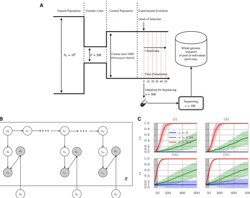
Consider a panmictic diploid population withfixed size ofN individuals. Letn¼ fntgt2Tbe the frequencies of the derived allele at generationst2 T for a given variant, where at gen-erationsT ¼ fti:0#t0,t1. . .,tTgsamples ofn individ-uals are chosen for pooled sequencing. The experiment is replicated R times. We denote allele frequencies of the R replicates by the setfngR:To identify the genes and variants that are responding to selection pressure, we use the follow-ing procedure:
1. Estimating population size: The procedure starts by esti-mating the effective population size,N^;under the assump-tion that much of the genome is evolving neutrally. 2. Estimating selection parameters: For each polymorphic
site, selection and dominance parameters s;h are esti-mated so as to maximize the likelihood of the time-series data, givenN^:
3. Computing likelihood statistics: For each variant, a log-odds ratio of the likelihood of selection modelðs.0Þto the likelihood of neutral evolution/drift model is com-puted. Likelihood ratios in a genomic region are combined to compute the CLEARstatistic for the region.
4. Hypothesis testing: An empirical null distribution of the CLEAR statistic is calculated using genome-wide drift
simulations, and used to computeP-values and thresholds for a specified false discovery rate (FDR). We perform single-locus hypothesis testing within selected regions to identify significant variants and report genes that intersect with the selected variants.
These steps are described in detail below.
Estimating population size
Methods for estimating population sizes from temporal neutral evolution data have been developed (Williamson and Slatkin 1999; Anderson et al. 2000; Bollback et al. 2008; Terhorst et al.2015; Jónás et al.2016). Here, we aim to extend these models to explicitly model the sam-pling noise that arise in pool-seq data. Specifically, we model the variation in sequence coverage over different locations, and the noise due to sequencing only a subset of the individuals in the population. In addition, many existing methods (Bollbacket al.2008; Federet al.2014; Terhorst et al. 2015; Topaet al. 2015) are designed for large populations, and model frequency as a continuous quantity. We observed that using Brownian motion to model frequency drift may be inadequate for small popu-lations, low starting frequencies, and sparse sampling (in time); factors that are common in experimental evolution (seeResults, Figure 3, A–C, and Figure 2). To this end, we model the Wright–Fisher Markov process for generating pool-seq data (Supplemental Material, Figure S1 in File
S3) via a discrete HMM (Figure 1B). We start by comput-ing a likelihood function for the population size given neu-tral pool-seq data.
Likelihood for the neutral model: We model the allele frequency counts 2Nnt as being sampled from a binomial distribution. Specifically,
n0p;
2Nntjnt21binomialð2N;nt21Þ;
where pis the global distribution of allele frequencies in the base population. Note that p depends on the demo-graphic history of the founder lines and can be estimated from the site-frequency spectrum (see Figure S2 inFile S3) of the initial population. For notational convenience, henceforth we omit the dependence of likelihoods to the parameterp.
To estimate frequency after ttransitions, it is enough to specify the 2N32Ntransition matrixPðtÞ;wherePðtÞ½i;j
de-notes probability of change in allele frequency fromi=2Nto j=2Nintgenerations:
Pð1Þ½i;j ¼Pr
ntþ1¼ j
2N
nt¼ i
2N
¼ 2N j
!
sntjð12ntÞ2N2j;
(1)
PðtÞ¼Pðt21ÞPð1Þ: (2)
Furthermore, in an E&R experiment, n#N individuals are randomly selected for sequencing. The sampled allele fre-quencies,fytgt2T;are also binomially distributed:
2nytbinomialð2n;ntÞ: (3)
We introduce the 2N32n sampling matrixY, whereY½i;j stores the probability that the sample allele frequency isj=2n given that the true allele frequency isi=2N:
We denote the pool-seq data for that variant as fxt¼ hct;dtigt2T; where dt andct represent the coverage and the read count of the derived allele, respectively. Let fltgt2T be the sequencing coverage at different generations. Then, the observed data are sampled according to
dtPoissonðltÞ; ctbinomialðdt;ytÞ: (4)
The emission probability for an observed tuplext¼ hdt;ctiis
eiðxtÞ ¼
dt ct
i 2n
ct 1 2 i
2n
dt2ct
: (5)
For 1#t#T; 1#j#2N;let at;j denote the probability of emitting x1;x2;. . .;xt and reaching state j at tt: Then, at can be computed using the forward procedure (Durbin et al.1998):
where dt¼tt2tt21: The joint likelihood of the observed
data fromRindependent observations is given by
LðNjfxgR;nÞ ¼ QR r¼1L
NjxðrÞ;n¼Prðfxg RjN;nÞ
¼ QR r¼1
P i a
ðrÞ T;i
(7)
wherex¼ fxtgt2T:The graphical model and the generative process for which data are being generated is depicted in Figure 1B and Figure S1 inFile S3, respectively.
Finally, the last step is to compute an estimate N^ that maximizes the likelihood of allMvariants in the whole
ge-nome. LetxðirÞdenote the time-series data of theith variant in replicater. Then,
^
N¼arg max
N YM
i¼1 YR
r¼1
LhNjxðirÞi: (8)
Estimating selection parameters
Likelihood for the selection model:Assume that the site is evolving under selection constraintss2ℝandh2ℝþ;where sandhdenote selection strength and dominance parameters, respectively. By definition, the relativefitness values of geno-types 0|0, 0|1, and 1|1 are given byw00¼1;w01¼1þhs;
Figure 1 E&R selection experiments onD. melanogaster. (A) Typical configuration in which time-series data are collected forD. melanogaster. A small set of founder linesðF¼200Þis selected from a large populationðNo¼106Þ;and used to create a subpopulation of isofemale lines. Multiple
andw11¼1þs:Then,ntþ;the frequency at timettþ1 (one generation ahead), can be estimated using:
^
ntþ¼E½ntþjs;h;nt ¼ w11n 2
t þw01ntð12ntÞ w11n2t þ2w01ntð12ntÞ þw00ð12ntÞ2
¼ntþ
sðhþ ð122hÞntÞntð12ntÞ
1þsnt½2hþ ð122hÞnt :
(9)
The machinery for computing likelihood of the selection parameters is identical to that of population size, except for transition matrices. Hence, here we only describe the defi ni-tion transini-tion matrixQs;hof the selection model. LetQðst;hÞ½i;j denote the probability of transition fromi=2Ntoj=2Nin
t generations, then (see Ewens 2004, p. 24, equations 1.58–1.59):
Qð1Þs;h½i;j ¼Pr
ntþ ¼ j
2N
nt¼ i
2N;s;h;N
¼ 2N j
!
^
ntjþð12^ntþÞ2N2j
(10)
Qsðt;hÞ¼Qðs;th21ÞQð1Þs;h: (11)
The maximum likelihood estimates are given by
^s;h^¼arg max
s;h YR
r¼1
Ls;hjxðrÞ;N^
: (12)
Using grid search, we first estimateN(Equation 8), and subsequently, we estimate parameterssandh(Equation 12, Figure S3 inFile S3). By broadcasting and vectoriz-ing the grid search operations across all variants, the genome scan on millions of polymorphisms can be done in a significantly smaller time than iterating a numerical optimization routine for each variant (see Results and Figure 6).
Empirical likelihood-ratio statistics
The likelihood-ratio statistic for testing directional selection, to be computed for each variant, is given by
H¼22log Lðs;0:5jfxgR;NÞ^ Lð0;0:5jfxgR;NÞ^
; (13)
where s¼arg max s
QR
r¼1Lðs;0:5jxðrÞ;NÞ^ :Similarly, we can
define a test statistic for testing if selection is dominant by
Figure 2 Comparison of empirical distributions of allele frequencies (red)vs.predictions from Brownian motion (green), and Markov chain (blue). Comparison of empirical and theoretical distributions under neutral evolution (A–F) and selection (G–M) with different starting frequencies
D¼22log Lð^s;^hjfxgR;NÞ^ Lðs;0:5jfxgR;NÞ^
: (14)
While extending the single-locus Wright–Fisher model to multiple linked loci can improve the power of the model (Terhorstet al.2015), it is computationally and statistically expensive to compute exact likelihood. In addition, comput-ing linked-loci joint likelihood requires haplotype resolved data, which pool-seq does not provide. Here, similar to Nielsenet al.(2005), we calculate the composite-likelihood-ratioscore for a genomic region,
H ¼ 1 jLj
X
ℓ2L
Hℓ; (15)
where L is a collection of segregating sites and Hℓ is the likelihood-ratio score based for each variant ℓin L. The optimal value of the hyper-parameterLdepends upon a num-ber of factors, including initial frequency of the favored allele, recombination rates, linkage of the favored allele to neigh-boring variants, population size, coverage, and time since the onset of selection (duration of the experiment). InFile S3, we provide a heuristic to compute a reasonable value ofL, based on experimental data.
We work with a normalized value ofH;given by
H* i ¼
Hi2mC
sC ; "i2 C; (16)
wheremCandsCare the mean and standard deviation ofH values in a large regionC:We found different chromosomes have different distributions ofHi values, and therefore de-cided to use single chromosomes asC:
Hypothesis testing
Single-locus tests:Under neutrality, log-likelihood ratios can be approximated byx2distribution (Williams and Williams 2001), and P-values can be computed directly. However,
Federet al.(2014) showed that when the number of inde-pendent samples (replicates) is small,x2is a crude approxi-mation to the true null distribution and results in more false positives. Following their suggestion, we first compute the empirical null distribution using simulations with the esti-mated population size (see Figure S1 inFile S3). The empir-ical null distribution of statisticHis used to computeP-values as the fraction of null values that exceed the test score. Fi-nally, we use the method of Storey and Tibshirani (2003) to control for FDR in multiple testing.
Composite likelihood tests:Similar to single-locus tests, we compute the null distribution of theH* statistic using whole-genome simulations with the estimated population size, and subsequently compute the FDR. The simulations for generat-ing the null distribution ofH* are described next.
Simulations
We use the same simulation procedure for two purposes. First, we use the simulations to test the power of CLEARagainst other
methods in small genomic windows. Second, we use them to generate the distribution of null values for the statistic to com-pute empiricalP-values. We mainly chose parameters that are relevant to D. melanogaster experimental evolution (Kofler and Schlötterer 2013). See also Figure 1A for illustration.
1. Creating initial founder line haplotypes: Using msms (Ewing and Hermisson 2010), we created neutral popu-lations forFfounding haplotypes with command $./msms hFi12th2mWNoi2rh2rWNoi hWi, whereF¼200 is the number of founder lines,No¼106is the effective founder population size,r¼231028 is the recombination rate, andm¼231029 is the mutation rate. The window size Wis used to compute u¼2mNoW and r¼2NorW: We choseW= 50 kbp for simulating individual windows for performance evaluations, andW= 20 Mbp for simulating D. melanogasterchromosomes forP-value computations. 2. Creating initial diploid population: An initial set ofF¼200
haplotypes was created from step 1, and duplicated to
createFhomozygous diploid individuals to simulate gener-ation of inbred lines.Ndiploid individuals were generated by sampling with replacement from theFindividuals. 3. Forward simulation: We used forward simulations for
evolving populations under selection. We also consider selection regimes in which the favored allele is chosen from standing variation (notde novo mutations). Given initial diploid population, position of the site under selec-tion, selection strengths, number of replicatesR¼3; re-combination rate r¼231028; and sampling times T ¼ f0;10;20;30;40;50g; simuPop (Peng and Kimmel 2005) was used to perform the forward simulation and compute allele frequencies for all of theRreplicates. For hard sweep (respectively, soft sweep) simulations we ran-domly chose a site with an initial frequency ofn0¼0:005 (respectively,n0¼0:1Þto be the favored allele. For gen-erating the null distribution with drift forP-value compu-tations, we used this procedure withs¼0:
4. Sequencing simulation: Given allele frequency trajecto-ries we sampled depth of each site in each replicate iden-tically and independently from Poisson (l), where
l2 f30;100;300g is the coverage for the experiment. Once depthdis drawn for the site with frequencyn, the number of readsccarrying the derived allele are sampled according to binomialðd;nÞ: For experiments withfinite depth the tuplehc;diis the input data for each site.
Data availability
The source code and running scripts for CLEARare publicly
available athttps://github.com/airanmehr/clear.
D. melanogasterdata was originally published (Orozco-ter Wengelet al.2012; Franssenet al.2015). The data set of the
D. melanogasterstudy, until generation 37, is obtained from the Dryad digital repository (http://datadryad.org) under accession DOI: 10.5061/dryad.60k68. Generation 59 of the D. melanogaster study is accessed from the European Se-quence Read Archive (http://www.ebi.ac.uk/ena/) under the project accession number PRJEB6340. The data set con-taining the experimental evolution of yeast populations (Burkeet al.2014) is downloaded fromhttp://wfitch.bio.uci. edu/tdlong/PapersRawData/BurkeYeast.gz(last accessed January 24, 2017). University of California, Santa Cruz browser tracks forD. melanogasterand yeast data analysis are found in File 1 and File 2, respectively.
Results
Modeling allele frequency trajectories in small populations
Wefirst tested the goodness offit of the discretevs.Brownian motion (a continuous-state model) in modeling allele fre-quency trajectories, under general E&R parameters. For this purpose, we conducted 100 K simulations with two time samplesT ¼ f0;tgwheret2 f1;10;100gis the parameter controlling the density of sampling in time. In addition, we repeated simulations for different values of starting fre-quencyn0 2 f0:005;0:1g(i.e., hard and soft sweep) and se-lection strength s2 f0;0:1g (i.e., neutral and selection). Then, given initial frequencyn0;we computed the expected distribution of the frequency of the next samplentunder two
models to make a comparison. Figure 2, A–F, shows that Brownian motion (continuous model) is inadequate whenn0 is far from 0.5, or when sampling times are sparseðt.1Þ:If the favored allele arises from standing variation in a neutral population, it is unlikely to have a frequency close to 0.5, and
the starting frequencies are usually much smaller (see Figure S2 in File S3). Moreover, in typicalD. melanogaster experi-ments, for example, sampling is sparse. Often, the experiment is designed so that 10#t#100(Zhouet al.2011; Orozco-ter Wengel et al. 2012; Kofler and Schlötterer 2013; Franssen et al.2015).
In contrast to the Brownian motion approximation, dis-crete Markov chain predictions (Equation 11) are highly consistent with empirical data for a wide range of simulation parameters (Figure 2, A–M). Moreover, the discrete Markov chain can be modified to model the case when the the allele is under selection.
Detection power
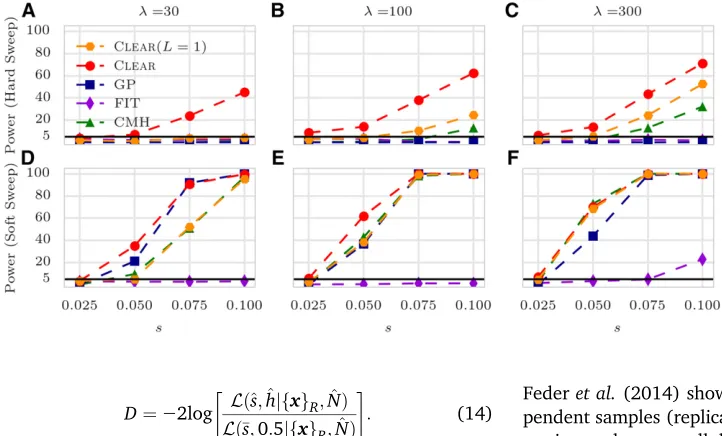
We compared the performance of CLEARagainst other
meth-ods for detecting selection. For each method we calculated detection power as the percentage of true positives identified with a false-positive rate #0:05: For each configuration (specified with values for selection coefficients, starting allele frequencyn0;and coveragel), the power of each method is evaluated over 2000 distinct simulations, half of which modeled neutral evolution and the rest modeled positive selection.
We compared the power of CLEARwith GP (Terhorstet al.
2015), FIT (Federet al.2014), and CMH (Agresti and Kateri
2011) statistics. FIT and GP convert read counts to allele frequencies prior to computing the test statistic. CLEARshows
the highest power in all cases and the power stays relatively high even for low coverage (Figure 3 and Table S1 inFile S3). In particular, the difference in performance of CLEARwith
other methods is pronounced when starting frequency is low. The advantage of CLEARstems from the fact that the
Figure 6 Running time. Box plots of running time per variant (CPU sec-onds) of CLEARðHÞ;CMH, FIT, and GP with 1, 3, 5, 7, and 10 loci over 1000 simulations conducted on a workstation with Intel Core i7 proces-sor. The average running time for each method is shown on thex-axis. In all simulations, three replicates are evolved and sampled at generations T ¼ f0;10;20;30;40;50g.
Figure 5Distribution of bias for 1003
favored allele with a low starting frequency might be missed by low coverage sequencing. In this case, incorpo-rating the signal from linked sites becomes increasingly important. We note that methods using only two time points, such as CMH, do relatively well for high selection values and high coverage. However, the use of time-series data can increase detection power in low coverage exper-iments or when the starting frequency is low. Moreover, time-series data provide means for estimating selection parameterssandh(see below). Finally, as CLEARis robust
to change of coverage, our results (Figure 3, B and C) suggest that taking many samples with lower coverage is preferable to sparse sampling with higher coverage. For comparison purposes, we also tested CLEARusing the
single-locus statistic ðL¼1Þ: For the most part, CLEAR
showed an improvement over other methods even with L¼1;or showed similar performance. The performance improved with higherL.
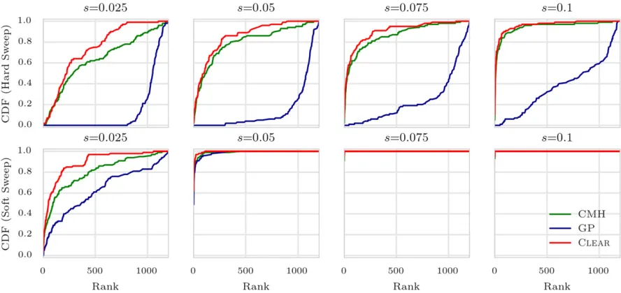
Site identification
In general, localizing the favored variant using pool-seq data is a nontrivial task due to extensive linkage disequilibrium (LD) (Tobler et al. 2014). To measure performance, we sorted variants by theirHscores and computed rank of the favored allele for each method. For each setting ofn0ands, we conducted 1000 simulations and computed the rank of the favored mutation in each simulation. The cumulative distribution of the rank of the favored allele in 1000 simula-tions for each setting (Figure 4) shows that CLEAR
outper-forms other statistics.
An interesting observation is revisiting the contrast be-tween site identification and detection (Long et al. 2013; Tobleret al.2014). When selection strength is high, detection is easier (Figure 3, A–F), but site identification is harder, due to the high LD between flanking variants and the favored allele (Figure 4, A–F). Moreover, site identification becomes more difficult whenever the initial frequency of the favored allele is low; i.e., at the onset of selection, LD between a favored allele and its nearby variants is high. For example, when coveragel¼100 and selection coefficients¼0:1;the
detection power is 75% for hard sweep, but 100% for soft sweep (Figure 3, B–E). In contrast, the favored site was ranked as the top in 14% of hard sweep cases, compared to 95% of soft sweep simulations.
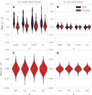
Estimating parameters
CLEAR estimates effective population size N^ and selection
parameters,^sandh^, as a byproduct of the hypothesis test-ing. We computed bias of selectionfitnessðs2^sÞand dom-inanceðh2^hÞfor CLEARand GP for 1000 simulations in each
setting. The distribution of the error (bias) for 1003 cover-age is presented in Figure 5 for different configurations. Figures S4 and S5 in File S3 provide the distribution of estimation errors for 303and 3003coverage, respectively. For hard sweep, CLEARprovides estimates of swith lower variance of bias (Figure 5A and Figure S6 inFile S3). In soft sweep, GP and CLEARboth provide unbiased estimates ofs
with low variance (Figure 5B). Figure 5, C and D, shows that CLEAR provides unbiased estimates of h as well when
h2 f0;0:5;1;2g and s¼0:1:We also tested if CLEAR
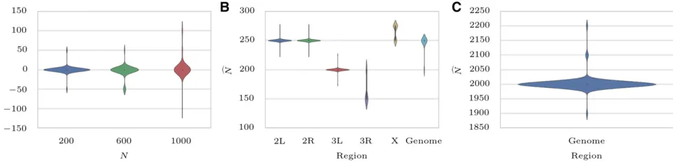
pro-vides unbiased estimates ofNby estimating population size on 1000 simulations whenN2 f200;600;1000g:As shown in Figure 7A and Figure S9, A–C, inFile S3maximum likeli-hood is attained at the true value of the parameter.
Running time
As CLEARdoes not compute exact likelihood of a region (i.e.,
does not explicitly model linkage between sites), the com-plexity of scanning a genome is linear in the number of poly-morphisms. Calculating the score of each variant requires an OðTRN3Þ computation for H:However, most of the opera-tions are can be vectorized for all replicates to make the effective running time for each variant faster. We conducted 1000 simulations and measured running times for computing site statisticsH, FIT, CMH, and GP with different numbers of linked loci. Our analysis reveals (Figure 6) that CLEARis or-ders of magnitude faster than GP, and comparable to FIT. While slower than CMH on the time per variant, the actual running times are comparable after vectorization and broad-casting over variants (see below).
These times can have a practical consequence. For instance, to run GP in the single-locus mode on the entire pool-seq data of theD. melanogastergenome from a small sample (1.6-M variant sites), it would take 1444 CPU hours (1 CPU month). In contrast, after vectorizing and broadcasting oper-ations for all variant operoper-ations using the numba package, CLEARtook 75 min to perform a scan, including precomputa-tion; while the fastest method, CMH, took 17 min.
Analysis of Real Data
Analysis of a D. melanogaster adaptation to alternating temperatures:We applied CLEARto the data from a study of
the adaptation of D. melanogaster to alternating tempera-tures (Orozco-ter Wengelet al.2012; Franssenet al.2015), where three replicate samples were chosen from a population ofD. melanogasterfor 59 generations under alternating 12-hr cycles of hot-stressful (28) and nonstressful (18) tempera-tures, and sequenced. In this data set, sequencing coverage is different across replicates and generations (seefigure S2 of Terhorst et al. 2015) which makes variant depths highly heterogeneous (Figure S10 inFile S3).
We first filtered out heterochromatic, centromeric, and telomeric regions (Fiston-Lavieret al.2010), and those var-iants that have a collective coverage of.1500 in all 13 pop-ulations: three replicates at the base population, two
replicates at generation 15, one replicate at generation 23, one replicate at generation 27, three replicates at generation 37, and three replicates at generation 59. Afterfiltering, we ended up with 1,605,714 variants.
Next, we estimated genome-wide population sizeN^ ¼250 (Figure 7B and Figure S9E inFile S3), which is consistent with previous studies (Orozco-ter Wengelet al.2012; Jónás et al. 2016). The likelihood curves of CLEAR are sharper around the optimum compared to that of the method of Bollback et al.(2008) (seefigure S1 in Orozco-ter Wengel et al. 2012). Also, chromosomes3L and3R appear to have a smaller population size, N^¼200; and 150; respectively. Others have made similar observations on this data. In par-ticular, Jónáset al.(2016) showed that the chromosome-wise population size varies even more when it is computed for each replicate separately (see table 1 in Jónáset al.2016). For instance,N^is 131 for chromosome3R replicate 1, while it is 328 for chromosomeXreplicate 2.
While it would be ideal to compute the CLEARstatistic for
each replicate and chromosome separately, computing em-pirical P-values and significant regions become computa-tionally intensive as the empirical null distribution of each replicate and each chromosome needs to be computed. Hence, we use a single genome-wide estimateN^ ¼250 in all analyses, but we normalize statistic H* separately for each chromosome.
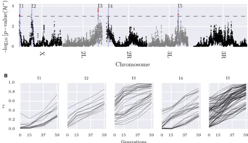
We used a heuristic calculation (seeFile S3) to choose the sliding window sizeLas the distance where the LD between the favored mutation and a siteL=2-bp away remains strong. ForD. melanogasterparameters, we obtainedL¼30 kbp: We computed the normalized test statisticH* on sliding win-dows of size of 30 kbp and step size of 5 kbp over the genome (see Figure 8A).
The empirical null distribution of H* was estimated by creating 100 whole-genome simulations (400 K statistic val-ues), as described inMaterial and Methods. Then, theP-value of the test statistic in each region in the experimental data was calculated as the fraction of the null statistic values that are greater than or equal to the test statistic(see Figure S11 in
File S3). After correcting for multiple testing, we identified
five contiguous intervals (Figure 8) satisfying FDR#0:05; and covering 2829 polymorphic sites. We further performed single-locus hypothesis testing on the 2829 sites to identify 174 individual variants with an FDR#0:01 (Figure 8B).
Thefinal set of 174 variants fall within 32 genes (Table S3 inFile S3), including many serine inhibitory proteases (ser-pins) and other genes involved in endocytosis. Recycling of synaptic vesicles is seen to be blocked at high temperature in temperature-sensitive Drosophila mutants (Kosaka and Ikeda 1983). This is also supported by gene ontology (GO)-enrichment analysis, where a single GO term “inhibition of proteolysis” is found to be enriched (corrected P-value = 0.0041). To test for dominant selection, we computed the D statistic on simulated neutral and experimental data, and computedP-values accordingly. After correcting for multiple testing, 96 variants were discovered with an FDR#0:01 (Fig-ure S12 inFile S3).
Analysis of outcrossing yeast populations
We also applied CLEARto 12 replicate samples of outcrossing
yeast populations (Burkeet al.2014), where samples were taken at generationsT ¼ f0;180;360;540gWe observed a significant variation in the genome-wide, site-frequency spec-trum of certain populations over different time points for some replicates (Figure S13 inFile S3). The variation does not have an easily identifiable cause. Therefore, we focused analysis on seven replicatesr2 f3;7;8;9;10;11;12gwith a
genome-wide, site-frequency spectrum over the time range (Figure S14 inFile S3).
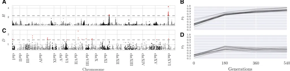
We estimated population size to beN^ ¼2000 haplotypes (Figure 7C and Figure S9F inFile S3), and computed the^s;^h; andHstatistics accordingly. To computeP-values, we created 1-M single-locus neutral simulations according to the exper-imental data’s initial frequency and coverage. By setting the FDR cutoff to 0.05, only 18 and 16 variants show significant signal for directional and dominant selection, respectively (Figure 9 S12 inFile S3). Selected variants for directional selection are clustered in two regions, which match two of thefive regions (regions C and E infigure 2A in Burkeet al.2014) identified by Burkeet al.(2014) in their preliminary analysis. UCSC browser tracks for analysis of D.melanogasterand Yeast datasets are avail-able asFile S1andFile S2, respectively.
Discussion
We developed a computational tool, CLEAR, that can detect regions
and variants under selection E&R experiments. Using extensive sim-ulations, we show that CLEAR outperforms existing methods in
detecting selection, locating the favored allele, and estimating model parameters. Also, while being computationally efficient, CLEAR pro-vides a means for estimating populations size and hypothesis testing. Many factors; such as small population size,finite coverage, LD,finite sampling for sequencing, duration of the experiment, and the small number of replicates; can limit the power of tools for analyzing E&R. Here, by discrete modeling, CLEARestimates
population size and provides unbiased estimates ofsandh. It adjusts for heterogeneous coverage of pool-seq data, and ex-ploits the presence of linkage within a region to compute a composite likelihood ratio statistic.
It should be noted that, even though we described CLEARfor
smallfixed-size populations, the statistic can be adjusted for other scenarios, including changing population sizes when the demography is known. For large populations, transitions can be computed on sparse data structures, as for largeNthe transition matrices become increasingly sparse. Alternatively, frequencies can be binned to reduce dimensionality.
The comparison of hard- and soft-sweep scenarios showed that the initial frequency of the favored allele can have a
nontrivial effect on the statistical power for identifying selec-tion. Interestingly, while it is easier to detect a region un-dergoing strong selection, it is harder to locate the favored allele in that region.
There are many directions to improve the analyses pre-sented here. In particular, we plan to focus our attention on other organisms with more complex life cycles, experiments with variable population size, and longer sampling-time spans. As E&R experiments continue to grow, deeper insights into adaptation will go hand in hand with improved compu-tational analysis.
Acknowledgments
The authors thank the anonymous reviewers whose com-ments substantially improved the quality and clarity of this manuscript. A.I., A.A., and V.B. were supported by grants from the National Institutes of Health (1R01 GM-114362) and National Science Foundation (DBI-1458557 and IIS-1318386). C.S. is supported by the European Research Council grant ArchAdapt. V.B. is a cofounder, has an equity interest, and receives income from Digital Proteomics, LLC (DP). The terms of this arrangement have been reviewed and approved by the University of California, San Diego in accordance with its conflict of interest policies. DP was not involved in the research presented here.
Literature Cited
Agresti, A. Categorical Data Analysis, Ed. 2, inWiley Series in Prob-ability and Statistics. Wiley-Interscience, July 2002.
Anderson, E. C., E. G. Williamson, and E. A. Thompson, 2000 Monte Carlo evaluation of the likelihood for Ne from temporally spaced samples. Genetics 156: 2109–2118.
Ariey, F., B. Witkowski, C. Amaratunga, J. Beghain, A.-C. Langlois
et al., 2014 A molecular marker of artemisinin-resistant Plas-modium falciparum malaria. Nature 505: 50–55.
Baldwin-Brown, J. G., A. D. Long, and K. R. Thornton, 2014 The power to detect quantitative trait loci using resequenced, exper-imentally evolved populations of diploid, sexual organisms.Mol. Biol. Evol.31: 1040–1055.
Barrett, R. D. H., S. M. Rogers, and D. Schluter, 2008 Natural selection on a major armor gene in threespine stickleback. Sci-ence 322: 255–257.
Barrick, J. E., and R. E. Lenski, 2013 Genome dynamics during experimental evolution. Nat. Rev. Genet. 14: 827–839. Barrick, J. E., D. S. Yu, S. H. Yoon, H. Jeong, T. K. Oh et al.,
2009 Genome evolution and adaptation in a long-term exper-iment with Escherichia coli. Nature 461: 1243–1247.
Bergland, A. O., E. L. Behrman, K. R. O’Brien, P. S. Schmidt, and D. A. Petrov, 2014 Genomic evidence of rapid and stable adaptive oscillations over seasonal time scales in Drosophila. PLoS Genet. 10: e1004775.
Bersaglieri, T., P. C. Sabeti, N. Patterson, T. Vanderploeg, S. F. Schaff-neret al., 2004 Genetic signatures of strong recent positive se-lection at the lactase gene. Am. J. Hum. Genet. 74: 1111–1120. Bollback, J. P., and J. P. Huelsenbeck, 2007 Clonal interference is
alleviated by high mutation rates in large populations. Mol. Biol. Evol. 24: 1397–1406.
Bollback, J. P., T. L. York, and R. Nielsen, 2008 Estimation of 2Nes from temporal allele frequency data. Genetics 179: 497–502.
Boyko, A. R., S. H. Williamson, A. R. Indap, J. D. Degenhardt, R. D. Hernandez et al., 2008 Assessing the evolutionary impact of amino acid mutations in the human genome. PLoS Genet. 4: e1000083.
Burke, M. K., J. P. Dunham, P. Shahrestani, K. R. Thornton, M. R. Roseet al., 2010 Genome-wide analysis of a long-term evolu-tion experiment with Drosophila. Nature 467: 587–590. Burke, M. K., G. Liti, and A. D. Long, 2014 Standing genetic variation
drives repeatable experimental evolution in outcrossing populations of Saccharomyces cerevisiae.Mol. Biol. Evol.31: 3228–3239. Daborn, P., S. Boundy, J. Yen, and B. Pittendrigh, and R.
ffrench-Constant, 2001 DDT resistance in Drosophila correlates with Cyp6g1 over-expression and confers cross-resistance to the ne-onicotinoid imidacloprid. Mol. Genet. Genomics 266: 556–563. Daniels, R., H.-H. Chang, P. D. Séne, D. C. Park, D. E. Neafseyet al., 2013 Genetic surveillance detects both clonal and epidemic transmission of malaria following enhanced intervention in Senegal. PLoS One 8: e60780.
Denef, V. J., and J. F. Banfield, 2012 In situ evolutionary rate measurements show ecological success of recently emerged bacterial hybrids. Science 336: 462–466.
Desai, M. M., and J. B. Plotkin, 2008 The polymorphism fre-quency spectrum offinitely many sites under selection. Genetics 180: 2175–2191.
Durbin, R., S. R. Eddy, A. Krogh, and G. Mitchison, 1998 Biological Sequence Analysis: Probabilistic Models of Proteins and Nucleic Acids. Cambridge University Press, Cambridge, United Kingdom. Ewens, W. J., 2004 Mathematical Population Genetics 1: Theoret-ical Introduction (Interdisciplinary Applied Mathematics, Vol. 27). Springer Science & Business Media, New York.
Ewing, G., and J. Hermisson, 2010 MSMS: a coalescent simula-tion program including recombinasimula-tion, demographic structure and selection at a single locus. Bioinformatics 26: 2064–2065. Fan, S., M. E. B. Hansen, Y. Lo, and S. A. Tishkoff, 2016 Going
global by adapting local: a review of recent human adaptation. Science 354: 54–59.
Feder, A. F., S. Kryazhimskiy, and J. B. Plotkin, 2014 Identifying sig-natures of selection in genetic time series. Genetics 196: 509–522. Feder, A. F., S.-Y. Rhee, S. P. Holmes, R. W. Shafer, D. A. Petrov
et al., 2016 More effective drugs lead to harder selective sweeps in the evolution of drug resistance in HIV-1. Elife 5: e10670 [corrigenda: Elife 6: e24879 (2017)].
Fiston-Lavier, A.-S., N. D. Singh, M. Lipatov, and D. A. Petrov, 2010 Drosophila melanogaster recombination rate calculator. Gene 463: 18–20.
Franssen, S. U., V. Nolte, R. Tobler, and C. Schlötterer, 2015 Patterns of linkage disequilibrium and long range hitchhiking in evolving experimental Drosophila melanogaster populations. Mol. Biol. Evol. 32: 495–509.
Gottesman, M. M., 2002 Mechanisms of cancer drug resistance. Annu. Rev. Med. 53: 615–627.
Hegreness, M., N. Shoresh, D. Hartl, and R. Kishony, 2006 An equivalence principle for the incorporation of favorable muta-tions in asexual populamuta-tions. Science 311: 1615–1617. Illingworth, C. J. R., and V. Mustonen, 2011 Distinguishing driver
and passenger mutations in an evolutionary history categorized by interference. Genetics 189: 989–1000.
Illingworth, C. J. R., L. Parts, S. Schiffels, G. Liti, and V. Mustonen, 2012 Quantifying selection acting on a complex trait using allele frequency time series data. Mol. Biol. Evol. 29: 1187–1197. Izutsu, M., A. Toyoda, A. Fujiyama, K. Agata, and N. Fuse,
2015 Dynamics of dark-fly genome under environmental se-lections. G3 (Bethesda) 6: 365–376.
Jónás, Á., T. Taus, C. Kosiol, C. Schlötterer, and A. Futschik, 2016 Estimating the effective population size from temporal allele frequency changes in experimental evolution. Genetics 204: 723–735.
Kawecki, T. J., R. E. Lenski, D. Ebert, B. Hollis, I. Olivieriet al., 2012 Experimental evolution. Trends Ecol. Evol. 27: 547–560. Kofler, R., and C. Schlötterer, 2013 A guide for the design of evolve and resequencing studies.Mol. Biol. Evol.31: 474–483. Kosaka, T., and K. Ikeda, 1983 Reversible blockage of membrane
retrieval and endocytosis in the Garland cell of the temperature-sensitive. J. Cell Biol. 97: 499–507.
Lang, G. I., D. Botstein, and M. M. Desai, 2011 Genetic variation and the fate of beneficial mutations in asexual populations. Ge-netics 188: 647–661.
Lang, G. I., D. P. Rice, M. J. Hickman, E. Sodergren, G. M. Weinstock
et al., 2013 Pervasive genetic hitchhiking and clonal interfer-ence in forty evolving yeast populations. Nature 500: 571–574. Levy, S. F., J. R. Blundell, S. Venkataram, D. A. Petrov, D. S. Fisher
et al., 2015 Quantitative evolutionary dynamics using high-resolution lineage tracking. Nature 519: 181–186.
Long, Q., F. A. Rabanal, D. Meng, C. D. Huber, A. Farlowet al., 2013 Massive genomic variation and strong selection in Arab-idopsis thaliana lines from Sweden. Nat. Genet. 45: 884–890. Malaspinas, A.-S., O. Malaspinas, S. N. Evans, and M. Slatkin,
2012 Estimating allele age and selection coefficient from time-serial data. Genetics 192: 599–607.
Maldarelli, F., M. Kearney, S. Palmer, R. Stephens, J. Micanet al., 2013 HIV populations are large and accumulate high genetic diversity in a nonlinear fashion. J. Virol. 87: 10313–10323. Martins, N. E., V. G. Faria, V. Nolte, C. Schlötterer, L. Teixeiraet al.,
2014 Host adaptation to viruses relies on few genes with dif-ferent cross-resistance properties. Proc. Natl. Acad. Sci. USA 111: 5938–5943.
Mathieson, I., and G. McVean, 2013 Estimating selection coeffi -cients in spatially structured populations from time series data of allele frequencies. Genetics 193: 973–984.
Nair, S., D. Nash, D. Sudimack, A. Jaidee, M. Barends et al., 2007 Recurrent gene amplification and soft selective sweeps during evolution of multidrug resistance in malaria parasites. Mol. Biol. Evol. 24: 562–573.
Nielsen, R., S. Williamson, Y. Kim, M. J. Hubisz, A. G. Clarket al., 2005 Genomic scans for selective sweeps using SNP data. Ge-nome Res. 15: 1566–1575.
Orozco-ter Wengel, P., M. Kapun, V. Nolte, R. Kofler, T. Flattet al., 2012 Adaptation of Drosophila to a novel laboratory environ-ment reveals temporally heterogeneous trajectories of selected alleles. Mol. Ecol. 21: 4931–4941.
Oz, T., A. Guvenek, S. Yildiz, E. Karaboga, Y. T. Tamer et al., 2014 Strength of selection pressure is an important parameter contributing to the complexity of antibiotic resistance evolution.
Mol. Biol. Evol.31: 2387–2401.
Peng, B., and M. Kimmel, 2005 simuPOP: a forward-time popula-tion genetics simulapopula-tion environment. Bioinformatics 21: 3686– 3687.
Pollak, E., 1983 A new method for estimating the effective popula-tion size from allele frequency changes. Genetics 104: 531–548. Reid, B. J., R. Kostadinov, and C. C. Maley, 2011 New strategies in
Barrett’s esophagus: integrating clonal evolutionary theory with clinical management. Clin. Cancer Res. 17: 3512–3519. Remolina, S. C., P. L. Chang, J. Leips, S. V. Nuzhdin, and K. A.
Hughes, 2012 Genomic basis of aging and life-history evolu-tion in Drosophila melanogaster. Evoluevolu-tion 66: 3390–3403.
Sawyer, S. A., and D. L. Hartl, 1992 Population genetics of poly-morphism and divergence. Genetics 132: 1161–1176.
Schlötterer, C., R. Kofler, E. Versace, R. Tobler, and S. U. Franssen, 2015 Combining experimental evolution with next-generation sequencing: a powerful tool to study adaptation from standing genetic variation. Heredity 114: 431–440.
Schraiber, J. G., S. N. Evans, and M. Slatkin, 2016 Bayesian in-ference of natural selection from allele frequency time series. Genetics 203: 493–511.
Simonson, T. S., Y. Yang, C. D. Huff, H. Yun, G. Qin et al., 2010 Genetic evidence for high-altitude adaptation in Tibet. Science 329: 72–75.
Spellberg, B., R. Guidos, D. Gilbert, J. Bradley, H. W. Boucheret al., 2008 The epidemic of antibiotic-resistant infections: a call to action for the medical community from the Infectious Diseases Society of America. Clin. Infect. Dis. 46: 155–164.
Steinrücken, M., A. Bhaskar, and Y. S. Song, 2014 A novel spectral method for inferring general diploid selection from time series genetic data. Ann. Appl. Stat. 8: 2203–2222.
Storey, J. D., and R. Tibshirani, 2003 Statistical significance for ge-nomewide studies. Proc. Natl. Acad. Sci. USA 100: 9440–9445. Terhorst, J., C. Schlötterer, and Y. S. Song, 2015 Multi-locus
anal-ysis of genomic time series data from experimental evolution. PLoS Genet. 11: e1005069.
Tobler, R., S. U. Franssen, R. Kofler, P. Orozco-terWengel, V. Nolte
et al., 2014 Massive habitat-specific genomic response in D. melanogaster populations during experimental evolution in hot and cold environments. Mol. Biol. Evol. 31: 364–375. Topa, H., Á. Jónás, R. Kofler, C. Kosiol, and A. Honkela,
2015 Gaussian process test for high-throughput sequencing time series: application to experimental evolution. Bioinfor-matics 31: 1762–1770.
Turner, T. L., A. D. Stewart, A. T. Fields, W. R. Rice, and A. M. Tarone, 2011 Population-based resequencing of experimen-tally evolved populations reveals the genetic basis of body size variation in Drosophila melanogaster. PLoS Genet. 7: e1001336. Wang, J., 2001 A pseudo-likelihood method for estimating effec-tive population size from temporally spaced samples. Genet. Res. 78: 243–257.
Waples, R. S., 1989 A generalized approach for estimating effec-tive population size from temporal changes in allele frequency. Genetics 121: 379–391.
Williams, D., 2001 Weighing the Odds: A Course in Probability and Statistics. Cambridge University Press, Cambridge, United Kingdom.
Williamson, E. G., and M. Slatkin, 1999 Using maximum likeli-hood to estimate population size from temporal changes in al-lele frequencies. Genetics 152: 755–761.
Winters, M. A., R. M. Lloyd, Jr., R. W. Shafer, M. J. Kozal, M. D. Milleret al., 2012 Development of elvitegravir resistance and linkage of integrase inhibitor mutations with protease and re-verse transcriptase resistance mutations. PLoS One 7: e40514. Yi, X., Y. Liang, E. Huerta-Sanchez, X. Jin, Z. X. P. Cuo et al.,
2010 Sequencing of 50 human exomes reveals adaptation to high altitude. Science 329: 75–78.
Zahreddine, H., and K. L. Borden, 2013 Mechanisms and insights into drug resistance in cancer. Front. Pharmacol. 4: 28. Zhou, D., N. Udpa, M. Gersten, D. W. Visk, A. Bashir et al.,
2011 Experimental selection of hypoxia-tolerant Drosophila melanogaster. Proc. Natl. Acad. Sci. USA 108: 2349–2354.