Estimating Allele Age and Selection Coefficient from Time-Serial Data

(1)

INVESTIGATION

Estimating Allele Age and Selection Coef

ﬁ

cient

from Time-Serial Data

Anna-Sapfo Malaspinas,*,1_{Orestis Malaspinas,}†,‡_{Steven N. Evans,}§_{and Montgomery Slatkin**} *Centre for Geogenetics, Natural History Museum of Denmark, University of Copenhagen, 1350 Copenhagen, Denmark,†Institut Jean le Rond d’Alembert, Université Pierre et Marie Curie, F-75252 Paris cedex 5, France,‡Computational Science Department, Centre Universitaire d’Informatique, Université de Genève, 1227 Carouge, Switzerland,§Department of Statistics, University of California, Berkeley California 94720-3860, and **Department of Integrative Biology, University of California, Berkeley, California 94720-3140

ABSTRACTRecent advances in sequencing technologies have made available an ever-increasing amount of ancient genomic data. In particular, it is now possible to target speciﬁc single nucleotide polymorphisms in several samples at different time points. Such time-series data are also available in the context of experimental or viral evolution. Time-time-series data should allow for a more precise inference of population genetic parameters and to test hypotheses about the recent action of natural selection. In this manuscript, we develop a likelihood method to jointly estimate the selection coefﬁcient and the age of an allele from time-serial data. Our method can be used for allele frequencies sampled from a single diallelic locus. The transition probabilities are calculated by approximating the standard diffusion equation of the Wright–Fisher model with a one-step process. We show that our method produces unbiased estimates. The accuracy of the method is tested via simulations. Finally, the utility of the method is illustrated with an application to several loci encoding coat color in horses, a pattern that has previously been linked with domestication. Importantly, given our ability to estimate the age of the allele, it is possible to gain traction on the important problem of distinguishing selection on new mutations from selection on standing variation. In this coat color example for instance, we estimate the age of this allele, which is found to predate domestication.

T

IME-series analysis is widespread in severalﬁelds, such as meteorology, economics, and physics (Hamilton 1994) with the relation being statistical models designed to deal with a time-ordered sequence of observations. Such obser-vations are also prevalent in several areas of biology. Until recently, however, time-series molecular data were only available for time spanning a few generations in higher or-ganisms. Therefore, in the context of population genetics, time-serial data were mostly limited to viral or experimental evolution (Wichmanet al.2005; Bollback and Huelsenbeck 2007; Nelson and Holmes 2007; Greshamet al.2008).

However, with recent advances in DNA sequencing and DNA preparation techniques, the study of extinct and long

dead organisms is now entering a new era, an era in which time-sampled measurements spanning hundreds or thou-sands of generations for even mammalian species may be obtained. For example, while previous studies were limited to short segments of mitochondrial DNA, whole nuclear genomes are now available from several ancient samples (Rasmussenet al.2010; Reichet al.2010), and it is now ad-ditionally possible to target speciﬁc DNA regions in ancient organisms (Lalueza-Foxet al.2007; Ludwiget al.2009; Rusk 2009). Therefore, time-serial data will become increasingly available for a whole range of organisms allowing one to test evolutionary questions using not only present day sam-ples, but also samples from extinct populations.

The relevant theory to describe such temporal changes in allele frequency has existed since the advent of population genetics (Fisher 1922; Wright 1931). Although not very common, several statistical methods and estimators to deal with time-serial data have been developed and applied to, for example, estimate historical changes in population size (Waples 1989; Williamson and Slatkin 1999; Anderson

et al.2000; Drummond and Rambaut 2007). More recently,

Manuscript received April 7, 2012; accepted for publication June 18, 2012 Supporting information is available online athttp://www.genetics.org/lookup/suppl/ doi:10.1534/genetics.112.140939/-/DC1.

1_{Corresponding author: Centre for Geogenetics, Natural History Museum of Denmark,}

(2)

in 2008, Bollbacket al.developed a method to coestimate the effective population size, Ne, and the selection coefﬁ

-cient, s, from temporal allele frequency data. They model the evolution of the allele frequency of a diallelic locus with a diffusion process that approximates a Wright–Fisher population genetic model (WF), under the assumption that the locus is under constant natural selection acting on dip-loid individuals.

Our work is a natural extension of Bollbacket al.’s (2008) method to also allow for the estimation of the allele age (i.e., the time since the mutational event),t0. Allele age is an

om-nipresent parameter in population genetics and along with the selection coefﬁcient it plays a crucial role in determining the sojourn time of a beneﬁcial mutation (see Slatkin and Rannala 2000 for a review). Additionally, given the recent focus on the important question of distinguishing between models of selection on newvs.standing mutations—a phe-nomenon that speaks to the fundamental mode and tempo of the process of adaptation—the ability to estimate the time of a mutational event is of paramount importance (see re-view of Barrett and Schluter 2008).

Our extension allows these competing models to be ad-dressed, unlike the previous work of Bollback et al.(2008) that assumed that at the ﬁrst time of sampling the popula-tion allele frequency was uniformly distributed. It follows from this latter assumption that even if the allele was not sampled at the oldest sampling time, it had to be present in the population. Here, we present an approach to coestimate

s,Ne, andt0by computing the likelihood of these parameters

for a suitable model.

In theTheorysection we explain how we approximate the WF model with a one-step process. We then discuss the nu-merical details of the implementation in both Numerics sec-tions. We show how our method performs on the basis of simulations in both Simulationssections. We analyze a data set of horses for the ASIPlocus for samples dating from the Pleistocene up to the present in bothReal datasections. We conclude and offer some further perspectives inConclusion.

Materials and Methods

Theory

We assume that there is a single, panmictic population evolving according to a WF population genetic model. Under this model, the frequency of an allele Ais a homogeneous discrete-time Markov chain. We denote the Markov chain describing the frequency of the allele A through time by

Xt. We assume that selection is constant from the time the

allele arose up to present. The allele under selection arises only once and there is no recurrent mutation. In other words, the only evolutionary forces acting on that allele are genetic drift and selection.

Selection is modeled as acting on diploid individuals. If we denote the two alleles byAanda, we can choose the geno-typicﬁtness to bewAA= 1 +s,wAa= 1 +sh, andwaa= 1,

where sis the selection coefﬁcient andh is the dominance

coefﬁcient (s. 21 andh2[0, 1]; see,e.g., Ewens 2004). If

Neis the effective population size, the states ofXtare the

allelic frequencies, with respect to the population size

xj¼j=2Ne for 0# j # 2Ne. Therefore, the state space is

f0;1=2Ne;. . .;ð2Ne21Þ=2Ne;1g. We deﬁne the rescaled

se-lection coefﬁcientg= 2Nes.

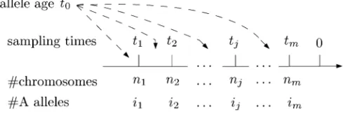
We compute the likelihood of the allele age t0, the

re-scaled selection coefﬁcientg, and the effective population sizeNe. To simplify the notation, deﬁneu[(g,Ne,t0) the

parameters of interest. Assume that we have samples from

mdistinct sampling time points. We suppose thatM= (n1,

n2,. . .,nm) chromosomes were collected, among whichI=

(i1,i2,. . .,im) are of theAtype, and that the chromosomes

were drawn at timesT= (t1,t2,. . .,tm), where time is

mea-sured in generations with tk21 , tk (see Figure 1). The

likelihood function of the parameters, for a given M and

h, isℓ(u) =p(i1,. . .,im|u,T).

To compute the likelihood, we can condition and sum over all the population allelic frequencies, xj1, . . ., xjm, at

each sampling timet1,t2,. . .,tm. We can then rewrite the

likelihood:

ℓðuÞ ¼X

j1

. . .X

jm

pi1;. . .;imju;T;xj1;xj2;. . .;xjmpxj1;xj2;. . .;xjmu;T: (1)

Conditional on the population allelic frequencies, the number ofAallelesijat each sampling time are independent of one

another. The ﬁrst term of the summation of Equation 1 becomes

pi1;. . .;imju;T;xj1;xj2;. . .;xjm

¼pi1jxj1

. . .pimjxjm

:

(2)

In the WF model the population is large and panmictic; therefore, we can assume that we sample the chromosomes with replacement and write fork2{0, ..,m}

pikjxjk

¼ nk ik

xik

jk

12xjk

nk2ik_:

(3)

SinceXtis a Markov chain, the second term of the

summa-tion of Equasumma-tion 1 is given by

pxj1;xj2;. . .;xjmu;T

¼pxjmxjm21;u;T

pxjm21xjm22;u;T

. . .pxj1xj0;u;T

;

(4)

Figure 1 Notation used throughout the text. The chromosomes M= (n1,n2,. . .,nm) are sampled at timesT= (t1,t2,. . .,tm) and there are

I= (i1,i2,. . .,im)Aalleles at each sampling time.

(3)

where xj0 is the frequency of the allele when it ﬁrst arose

in the population,i.e.,xj0¼1=2Ne. We can rewrite the

tran-sition probabilities of Xtpðxjkxjk21;u;TÞ ¼ptk2tk21ðxjk21;xjkÞ,

for a givenuandT. By substituting Equation 2 and 4 into 1 we obtain

ℓðuÞ ¼pði1;. . .;imju;TÞ5

P 2Ne

jm¼0 p

imj

jm

2Ne

X2Ne

jm21¼0 ptm2tm21

jm21 2Ne;

jm

2Ne

P 2Ne

jm21¼0 p

im21j

jm21 2Ne

X2Ne

jm22¼0 ptm212tm22

jm22 2Ne;

jm21 2Ne

⋯

p

i2j

j2 2Ne

X2Ne

j1¼0 pt22t1

j1 2Ne;

j2 2Ne

p

i1j

j1 2Ne

pt12t0

1 2Ne;

j1 2Ne

:

(5)

The solution for the transition probabilities for the nonneutral case of the WF model is elaborate (Ewens 2004 and citations therein, but see also Song and Steinrucken 2012). Rescaling the time by 2Ne, the Markov chain, Xt,

can be approximated by a diffusion process (“WF diffusion process”),Yt(see,e.g., Durrett 2008). Time is now in units

of 2Ne generations and is continuous and we replaceT by

T = (t1,. . .,tm), whereti¼ti=2Ne. The state space is also

continuous with states denoted by y 2 [0, 1]. This holds in the limit of large Ne, where X½t2Ne’Yt. The

transition densities of the diffusion process are denoted

pðykjyk21;u;T Þ ¼ptk2tk21ðyk21;ykÞ. In this article we further

approximate the diffusion process itself by a one-step pro-cess that we denoteZt(see,e.g., Van Kampen 1992). A

one-step process is a continuous-time Markov chain (i.e., discrete in space and continuous in time) where jumps are only allowed between two states that are adjacent to each other. As before, the states of the processZtare certain population

allelic frequencies that we denote by {z0, z1, . . ., zH21},

where His an integer. The states are chosen such that z0

and zH21are, respectively, the 0 and 1 allelic frequencies.

These are absorbing states since there is no recurrent muta-tion. The other states are chosen such that 0,zk,1 and zk21,zkfor 0,k,H21. The inﬁnitesimal generatorQ

of such a process is a tridiagonalH·Hmatrix. By denoting

bi(respectively,di) the rate of jumping to the right

(respec-tively, the left) of statei, we have that

Q¼ 0 B B B B B B B B @

0 . . . 0

d1 h1 b1 0

0 ⋱ ⋱ ⋱ 0 ⋮ ⋮

0 dk hk bk 0

⋮ 0 ⋱ ⋱ ⋱ 0

0 dH22 hH22 bH22

0 . . . 0 0

1 C C C C C C C C A ; (6)

wherehk=2(bk+dk). The transition probability between

two stateszjk21 andzjkof the process isptk2tk21ðzjk21;zjkÞ ¼

ðexpðQðtkþ12tkÞÞÞjk21;jk. With the appropriate choice ofbi

and di (see Supporting Information, File S1.1), one can

show that for large H,Zt ’Yt. In particular,bianddiwill

be functions ofzj,zj21,zj+1,gandh. Note thatYtis a

con-tinuous variable whereasZtis discrete. Therefore, choosing

yk21¼zjk21 andyk¼zjk;f0;1gwe have that

ptk2tk21ðyk21;ykÞ ’

ptk2tk21

zjk21;zjk

zjkþ12zjk21

2

¼ðexpðQðtk2tk21ÞÞÞjk21;jk

zjkþ12zjk21

2 ; (7)

where the denominator is necessary sinceYthas a

continuous-state space andZthas a discrete-state space. We can

approx-imate the likelihood described in Equation 5 by replacing the original process Xtby the one-step processZt. We then

have

ℓðuÞ ¼pði1;. . .;imju;T Þ5

P

H21

jm¼0 pimjzjm

PH21

jm21¼0 ptm2tm21

zjm21;zjm

P

H21

jm21¼0

pim21jzjm21

PH21

jm22¼0 ptm212tm22

zjm22;zjm21

⋯

pi2jzj2

PH21

j1¼0 pt22t1

zj1;zj2

pi1jzj1

pt12t0

₁

2Ne;

zj1

:

(8)

wherepðikjzjkÞ ¼ ð

nk

ikÞz

ik

jkð12zjkÞ

nk2ik _{from Equation 3.}

In the case of experimental evolution this unconditional process should be realistic since in principle one might want to estimate the selection coefﬁcient for any locus. We now consider one special case of what is presented above, motivated by ancient DNA data. We assume that the allele is segregating at the last sampling time (i.e., the process has not reached states 0 or 1). This case corresponds to what we think is a realistic scenario for how ancient DNA data would be collected, where presumably the locus of interest is poly-morphic at present. Indeed, only such loci would be selected for inference.

We can rewrite the resulting likelihood as

ℓC_ð_u_{Þ ¼}_p_i

1;. . .;imju;T;zjm;f0;1g

¼p

i1;. . .;im;zjm;f0;1gju;T

PH22

jm¼1 ptm2t0

1=2Ne;zjm

; (9)

where

pi1;. . .;im;zjm;f0;1gju;T

¼HP22

jm¼1

pimjzjm PH22

jm21¼1

ptm2tm21

zjm21;zjm

⋯

·pi2jzj2 PH22

j1¼0

pt22t1

zj1;zj2

·pi1jzj1pt12t0

1 2Ne;

zj1

:

(10)

We consider the subprocessZC

t deﬁned on the reduced state

space {z1, . . .,zH22}3{z0, z1. . . zH22, zH21}. The inﬁ

ni-tesimal generatorqC_{of such a process is the matrix}_Q

(4)

qC¼ 0 B B B B B B B B @

h₁ b₁ 0 . . . 0

d2 h₂ b₂ 0

0 ⋱ ⋱ ⋱ 0 ⋮

0 dk hk bk 0

⋮ ⋱ ⋱ ⋱ ⋱ 0

0 dH23 hH23 bH23

0 . . . 0 dH22 hH22

1 C C C C C C C C A : (11)

DenotingpC

tk2tk21ðzjk21;zjkÞthe transition probabilities of this

subprocess we have that ptk2tk21ðzjk21;zjkÞ ¼p

C

tk2tk21

ðzjk21;zjkÞ for " jk21;jk;f0;H21g(see File S1.2 for more

details).

Finally, to compute the likelihood of Equations 8 and 9, all that remains is to compute the matrix exponentiationeQt

andeqC_t

, respectively.

Numerics

We evaluate numerically the matrix exponentiation. The advantage of the current approach compared to Bollback

et al.’s is that we do not need to do a numerical integration step since the state space is alreadyﬁnite. The description of the matrix exponentiation is given inFile S1.2.

Although asymptotically the one-step process is equiva-lent to the WF model, since the state space ofZthas aﬁnite

number of states, the accuracy of the approximation depends on the choice of the states, or what we call from now on the

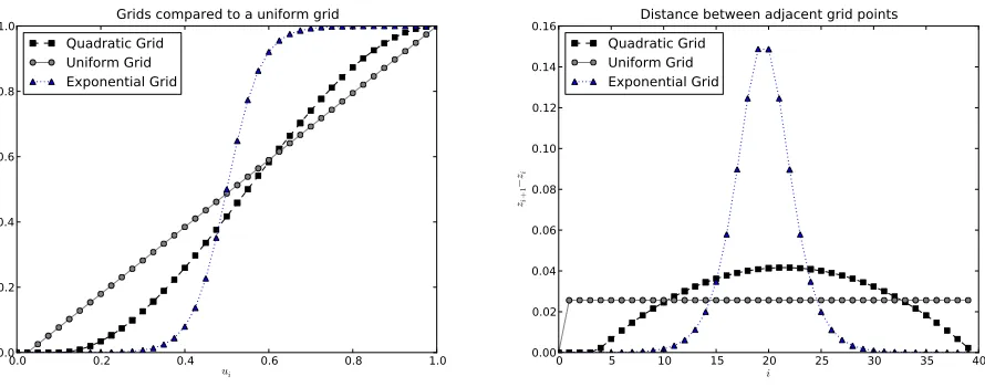
“grid.” We investigate three grids strongly inspired by Gutenkunstet al.(2009). Theﬁrst one is a uniform grid with a point added at 1=2Ne. The second and third grid are

a “quadratic grid”and an “exponential grid.” The last two grids were chosen to be reﬁned around the boundaries in such a way that the distance between adjacent points changes smoothly. The details for the grids are given inFile S1.2. All three grids have a point at 1=2Ne.

Since the likelihood function is complex, we were not able to compute the maximum of the function analytically. Therefore, to find the maximum, we first computed the likelihood over a large range of parameters. We verified that there is a single maximum for each time interval defined by adjacent sampling times,i.e., ift0,t1, the time intervals are

(2N,t0), (t1,t2),. . ., (tm21,tm), and the likelihood surface is

smooth. We used theSciPy(Joneset al.2001) implementa-tion of the Nelder–Mead simplex algorithm (Nelder and Mead 1965) toﬁnd the maximum for each time interval.

Our implementation is written inPythonandC++ mak-ing use of the Numpy (Oliphant 2006), SciPy, and mpack

(Nakata 2010) libraries for computations and of theMatplotlib

library (Hunter 2007) for plotting and is available upon request.

Simulations

To test our model, we simulate several data sets with the WF model forward in time. Simulating the WF model can be time consuming if the population size is large, so we picked a small population size (Ne = 500). In principle, however,

the conclusions hold for higher population size. We then

infer the maximum-likelihood estimates (MLEs) using our one-step method. We use two different sampling schemes. Theﬁrst one is similar to the real data set we analyze below,

i.e., 6 sampling times each with 50 chromosomes. The sec-ond one correspsec-onds to having twice as many sampling times with half the number of chromosomes, i.e., 12 sam-pling times and 25 chromosomes. We searched for the MLEs across aﬁnite domain,i.e.,Ne2[100, 1000],t02[23000,

0], and g 2 [2200, 200]. We assess the accuracy of our estimator and compare the sampling schemes by looking at the bias of the estimates and the root mean square error (RMSE).

Real data

In 2009, Ludwiget al.sequenced several loci encoding coat color in horses. Each locus has been shown to be linked with a color phenotype in present day horses. In other words, the phenotype associated with each locus is segregating in pres-ent populations. We reanalyze in this article one of the loci encoding for the agouti-signaling protein (ASIP), that con-trols the distribution of the black pigment (Rieder et al.

2001). We investigate the hypothesis that at the beginning of domestication some coat colors in horse were positively selected for.

The samples sequenced were obtained from Siberia, Middle and Eastern Europe, China, and the Iberian Penin-sula. As in Ludwiget al.(2009), we group the samples into six sampling times,t1’2000,t2’13100,t3’3700,t4’

2800,t5’1100, and t6’500 years BC. We assume that the

generation time of horses is 5 years, following Ludwiget al.

(2009). The wild-type horses are presumed to have been of bay color. The mutation of interest for theASIPlocus is re-cessive, since only horses homozygous for theASIPlocus will be black. We test for directional selection and seth= 0.

To compute a possible range for the population sizes we use data from Cieslaket al.(2010). They sequenced part of the control region of the mtDNA for 78 samples that are part of Ludwiget al.(2009)’s data set. The control region of the mtDNA is a noncoding region. One way to compute the population sizeNeis to compute the diversitypof the

sam-ples. Then, assuming the region is neutral and ignoring hitchhiking effects due to nearby selected sites, we use the relationship that relates the diversity of a sample to the population size,p¼2Nem⇒Ne¼p=2m, wheremis the

mu-tation rate per base pair per generation. To obtain an esti-mate of the mean and standard error of p of the mtDNA sample, we use the maximum-likelihood method imple-mented inMEGA(Tamuraet al.2011) with default param-eters. We approximate the standard error for the diversity by performing 1000 bootstraps. We use Jazin et al. (1998)’s estimate for the mutation rate (i.e.,m 2(3.0·1026_{, 4.4}_·

1025_{)). Jazin} _{et al.}_{(1998) used human families to obtain}

direct estimates of the mutation rate for mtDNA control region for a single generation. Although the mutation rate is an important parameter, we do not have direct estimate in horses and we have to rely on results for other species.

(5)

To obtain conservative upper/lower bounds forNewe use

the 95% conﬁdence interval (CI) bounds of the mutation rate and the diversity. If the CIs form and p are denoted (mlow,mup) and (plow,pup) respectively, we deﬁned

Nelow ¼ plow

2mup

and Neup ¼ pup

2mlow :

To ﬁnd the MLEs we use a domain deﬁned byNe 2 [200,

5000], t0 2 [210000, 0], and g 2 [2200, 200] for the

parameters. WeﬁxH= 400 for this computation.

For the CIs, several asymptotic results that apply for max-imum likelihood exist, especially for a time-serial Markov chain. Our sample sizes are generally small, however, so we chose to compute the CIs with a parametric bootstrap approach.

Note that several assumptions of our model are violated with this data set, such as constant population size and potentially random mating (since the samples are taken from all around the world); moreover, the MC1R locus, encoding a melanocortin receptor and related to the black pigment production, is known to have an epistatic interac-tion with ASIP(Rieder et al.2001). Nevertheless, we ana-lyze these data as described above to have a more direct comparison between our results with those obtained with Bollbacket al.’s method on the same data set.

Results and Discussion

Numerics

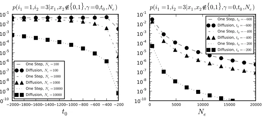
To validate the method, we compared several known ana-lytical results for the WF model with the one-step process. For the neutral case, it is possible to compute the likelihood since the transition probabilities are known for the diffusion process (see,e.g., Ewens 2004). As can be seen in Figure S3 (seeFile S1), even for a grid of size 100 the one-step process is a very good approximation of the diffusion process.

We also compare the relative error between the diffusion and the one-step process and demonstrate that when we increase the grid size the one-step process converges toward the diffusion process. The results for a particular choice of parameters is shown in Figure S4 (seeFile S1). We see that the one-step process does converge as expected with in-creasing grid size. In general we see that a quadratic grid and an exponential grid perform better than a uniform grid in general (see File S1.3 for details). In the applications below we use a quadratic grid of size between 100 and 400.

Simulations

We picked a population size ofNe= 500 and set the allele

age tot0=21400. Weﬁx the selection coefﬁcient to seven

potential values:g2{210,25, 0, 5, 10, 15, 20}.

First, we ﬁx the sampling times toT = (21000, 2800,

2600,2400,2200, 0) generations and sample 50 chromo-somes at each time point. Then we look at a scheme where the samples are taken every 100 generations from21100 up to 0 (i.e., 12 samples). At each sampling time we sample 25

chromosomes. The intent is to quantify whether it is better to sample more chromosomes at fewer time points, or the opposite.

The boxplot results for the MLEs for these simulations are shown on Figure 2. They are standard boxplots showing theﬁve-point summary (the minimum, theﬁrst quartile, the median, the third quartile, and the maximum). The plots for the bias and the RMSE are shown on Figure S5 (seeFile S1) for both schemes.

For the population size, the MLEs span all the potential range of Nevalues, but the bulk of the results exclude very

low population sizes. This suggests nevertheless that it is hard to estimate Ne with our method, at least with a

pre-cision higher than one order of magnitude. Our estimator is biased upward for both schemes but this might be explained by the presence of outliers since the median is largely accu-rate. Moreover, the second scheme, with fewer chromo-somes and more sampling times, leads to a smaller bias and a smaller RMSE for most cases. Intuitively, we think that most of the information to estimate scomes from the gen-eral trend of change in allele frequency, while most of the information to estimate Ne comes from the oscillations

around that general trend. In other words, to get a precise estimate ofNe, we need a dense sampling over time, which

is not the case for our simulations that we chose to match the real data setting.

In contrast, the results for the selection coefﬁcient are essentially unbiased, with a symmetric distribution, and the median matching the mean of the distribution. The variance remains large, and only whengis quite high can one reject neutrality. In particular, the higher the selection coefﬁcient, the higher the variance. The RMSE this time is worse for the second sampling scheme.

The results for the allele age also exhibit a large variance. The tail of the distribution is large. This can be explained by the use of the conditional process. Indeed for weak se-lection, if the number of derived alleles is high at the first sampling time the likelihood becomes uninformative for the allele age [i.e., the likelihood is flat for older allele ages; Figure S3 (see File S1)]. This leads to difficulties for the optimization algorithm to converge to the global maximum. The results seem to be systematically biased upward, al-though the median is accurate. For strong selection the like-lihood is more informative and the estimator is unbiased. Also, for strong selection the scheme with more samples through time performs considerably better. In conclusion, sam-pling fewer chromosomes over more samsam-pling times will lead to better results especially for strong selection in our examples.

Real data

(6)

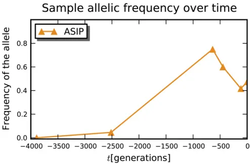
suggests a date of 3500 years BC (Outram et al. 2009), which would correspond to the third sampling time (i.e., when the sample frequencies start decreasing).

The ﬁrst step is to choose a potential range for the pop-ulation size. We foundp= 0.024 with a 95% CI of (0.018, 0.030). Together with the 95% CI of the mutation rate, this leads to a range forNeof (200, 5000). This is a small

pop-ulation size. It might be explained by the fact that the horses are a domesticated species and most samples are taken after the beginning of domestication, resulting in a smallNe. On

the other hand it might be that the mutation rate calculated for the human population for the control region is not ap-propriate for horses.

In Figure S6 (seeFile S1) we plot the likelihood surface for four values of Ne. This helps us conﬁrm that we have

found a global maximum. We note that the higher the pop-ulation size the higher the selection coefﬁcient and the older the allele age that maximize the likelihood. For example, if the population isﬁxed atNe= 200 thengmax=21.5 and

tmax

0 ¼ 22567. In contrast, if weﬁxNe= 5000, thengmax=

9.1 andtmax

0 ¼ 23550. In other words, if the mutation rate

is overestimated by, say, an order of magnitude, our poten-tial range for the population size will also be much higher.

Since there is no mutant allele at theﬁrst time of sampling, the allele might have arisen after theﬁrst sampling time. We denotedom1the range between (2N,23893] generations,

Figure 2Boxplots for the MLEs of each simulation repli-cate, for g 2{210, 25,. . ., 20},Ne = 400, andt0 = 21400. At the top is the scheme with 6 sampling times and 50 chromosomes sampled. At the bottom is the scheme with 12 sampling times and 25 chromosomes sampled. On each plot, the estimates for the population size,Ne(left), the rescaled selection coefﬁcient,g(middle), and the allele age,t0(right). For all subplots the triangle represents the mean of the estimates, and the circle rep-resents the true value. The rectangles of the boxplots are for theﬁrst and third quartiles and the black line repre-sents the median. The outliers are also indicated by crosses.

Figure 3 Change in allelic frequency over time for theASIPlocus. The sample sizes areM= (10, 22, 20, 20, 36, 38) and the number of derived alleles areI= (0, 1, 15, 12, 15, 18). The times have been offset so that the last sampling time is 0. Domestication is thought to have happened around 3500 years BC, which would correspond to around2600 gen-erations on this plot,i.e., the third sampling time.

(7)

and dom2the range (23893,22516]. As discussed before, the likelihood is therefore discontinuous as a function of the allele age with discontinuities at the sampling times. It is im-portant to look for the global maximum indom1anddom2

separately. Moreover, we compute the 95% CI indom1and in

dom2separately. We build the conﬁdence interval as a union of (potentially) disconnected domains.

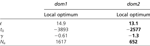
The values for the MLEs and 95% CI are shown in Table 1. Theﬁrst thing to note is that they are compatible with the results of Figure S6 (seeFile S1). The MLEs were found in

dom2: tmle

0 ﬃ 22600 with CI (24760, 23893] [ (23893,

2516],gmle_ﬃ₂_{1.3 with CI [}₂_{27.7, 60.7], and}_Nmle e ﬃ600

with CI [200, 5000] .

In Figure 4 we plot the distribution for the bootstrap rep-licates for each parameter and for the maximum-likelihood values. The conﬁdence interval was constructed as the inter-val between 2.5th and 97.5th percentile. We ran a total of 1400 replicates. For about 30 of those simulations, the opti-mizer did not converge. Among successful runs,500 did not have an MLE indom1ordom2and were discarded. From the remaining, about 823 were found indom2and 34 indom1.

The MLEs and the bootstrap results have several impli-cations. First, we do notﬁnd evidence for positive selection as could be anticipated by the archeological evidence for

domestication. The discrepancy between this study and Ludwiget al.(2009) isﬁrst the method used and second the parameter range assumed. Indeed, the results in Ludwig

et al. (2009) were obtained using Bollback et al. (2008)’s method. Since ourtmle

0 is indom2, and Bollbacket al.(2008)

assume that the allele was already present in theﬁrst time of sampling, it is to be expected that our results will be very different. Moreover, the potential range for the population size in Ludwiget al.(2009) is from 10,000 to 100,000;i.e., it does not overlap with the range forNethat we assume here.

As noted above, if we had assumed a larger population size, thegmle_{would be larger.}

The distribution of each parameter from the bootstrap replicates are almost unbiased relative to the true value (as could be expected from the results in the Simulation sec-tions). The distribution for g resembles a normal distribu-tion while the distribudistribu-tion forNeand t0are not as simple.

ForNe, the distribution is bimodal with a second mode at the

upper bound. This mode is a reﬂection of theﬁnite domain we impose on the search for the MLE rather than an actual mode. Similarly, fort0there is a mode at the lower bound for

dom2, an artifact of the bounds from the sampling times. As could be expected from the simulations above, the 95% CI forNesuggests that with these data we have little

ability to estimateNe, which we would expect from a sparse

sampling over time as discussed earlier. Similarly, we cannot distinguish between negative and positive selection asg’s CI is between 227.7 and 60.7. On the other hand, the boot-strap replicates suggest that the allele arose in dom2. We can indeed test the hypothesis that the allele age is not in

dom2; that is, we can test the null hypothesisH0:t0;dom2

vs.the alternative hypothesis that the allele age is indom2,

H1:t02dom2. We reject the null hypothesisH0withP-value

12823=ð823þ34Þ ¼0:04.

Table 1 Maxima for the ASIPlocus sequenced in Ludwig et al.

(2009)

dom1 dom2

Local optimum Local optimum

ℓ 14.9 13.1

t0 23893 22577

g 20.61 21.3

Ne 1617 652

The MLEs are in the rightmost column.

Figure 4 Bootstrap estimate of the sampling distribution of ML estimators of the three variablesNe,g,andt0for the parametric bootstrap. Out of 1400 simulations, 856 were compatible with the data (i.e., the maximum fort0was in

(8)

The domaindom2corresponds to 20,000 to 13,100 years BC. In other words, from the data, one could have already deduced that the allele had to be present before 213,100 years (i.e., before the presumed start of domestication). In-deed, domestication in horses is thought to have started about 3500 years BC (Outram et al. 2009). Our analysis shows that it is likely to have arisen within the last 20,000 years, thus clearly indicating that it was present as a standing variant at the time of domestication.

Conclusion

The allele age, the strength of selection, and the population size are all crucial parameters in population genetics. Although the volume of molecular data have been growing exponen-tially in recent years, it often remains a challenge to estimate those key parameters.

We develop a maximum-likelihood approach to estimating these parameters that deals with a particular type of data— temporal data. Our method is based on an approximation to the WF diffusion process and has the advantage of being quite

ﬂexible and appropriate for hypothesis testing. Moreover, it is fast for smallg, as one evaluation of the likelihood function takes 0.1 sec forg & 40 on a laptop with a i5 2.53 GHz CPU, for a data set like the one we analyze here.

We show through simulations that, for a sample of realistic size, although the variance of our estimator is quite large, our MLE is unbiased for estimating selection and is nearly unbiased for the age of the allele and the effective population size. On the other hand, our method is not appropriate for estimating the population size, even for simulations in which the model used to simulate the data matches the method used to infer the parameters. Indeed, for a realistic sampling scenario, the MLEs forNe, although unbiased, can

span several orders of magnitude. This is not surprising. The effective population size is a parameter notoriously difﬁcult to estimate, and our method considers only a single locus.

The sampling scheme has of course an impact on the ac-curacy of the estimator. We investigated two different sam-pling strategies and concluded that, in the cases considered, it is better to increase the number of sampling times rather than the number of samples per time point. It is indeed in-tuitive that to be able to estimate the allele age, for the con-ditional process, it is necessary to have a sample taken at a time close to the allele age. Indeed, in the conditional process, an allele will never getﬁxed or lost. Thus, after several units of rescaled time, the likelihood isﬂat.

We reanalyze a locus that was previously found to be under positive selection,ASIP, by evaluating samples rang-ing from the Pleistocene to the present. In this study, we test for directional selection and we do not have sufﬁcient reso-lution to distinguish positive from negative selection for this locus. This may be due to an insufﬁcient amount of data, but it could also be due to an underestimate of the effective population size, or a violation of one or more assumptions

of our null model, as discussed earlier. Although we are not able to estimate the selection coefﬁcient as precisely as we would like, we ﬁnd the age of the ASIP mutation to range between 20,000 to 13,100 years BC with an MLE at 13,400 years BC, which well predates domestication.

Even though we analyze a mammalian data set, our method can in principle be applied to data sets obtained in experimen-tal evolution or viral data. But, it is important to note that our approximation to the WF model will be valid only when the diffusion approximation to the WF model is appropriate, and hence only when 2Nesis not too large.

Importantly, our framework readily lends itself to being extended to multiple loci, the topic of future investigation. This extension is anticipated to provide greatly improved estimates ofNeand to permit the inference ofﬂuctuations in

historical population size—both issues of outstanding im-portance in gaining reﬁned estimates of selection coefﬁ -cients and allele age.

Acknowledgments

A.S.M. thanks Fernando Perez for help with the numerical analysis and Numpy, Scipy, Philip Johnson, and Emilia Huerta-Sanchez for helpful discussion. This work was part of A.S.M.’s Ph.D. thesis in the Department of Integrative Biology, University of California, Berkeley. It was funded in part by an Ernst and Lucie Schmidheiny fellowship to A.S. M., by the French Ministry of Industry (DGCIS) and the Region Ile-de-France in the framework of the LaBS Project, by a National Science Foundation grant DMS-0907630 to S.N.E., and by a National Institutes of Health grant (R01-GM40282) to M.S.

Literature Cited

Anderson, E. C., E. G. Williamson, and E. A. Thompson, 2000 Monte Carlo evaluation of the likelihood for Nefrom temporally spaced

samples. Genetics 156: 2109_–2118.

Barrett, R., and D. Schluter, 2008 Adaptation from standing ge-netic variation. Trends Ecol. Evol. 23(1): 38–44.

Bollback, J. P., and J. P. Huelsenbeck, 2007 Clonal interference is alleviated by high mutation rates in large populations. Mol. Biol. Evol. 24(6): 1397_–1406.

Bollback, J. P., T. L. York, and R. Nielsen, 2008 Estimation of 2Nes

from temporal allele frequency data. Genetics 179: 497–502. Cieslak, M., M. Pruvost, N. Benecke, M. Hofreiter, A. Moraleset al.,

2010 Origin and history of mitochondrial DNA lineages in do-mestic horses. PLoS ONE 5(12): e15311.

Drummond, A. J., and A. Rambaut, 2007 BEAST: Bayesian evo-lutionary analysis by sampling trees. BMC Evol. Biol. 7: 214. Durrett, R., 2008 Probability Models for DNA Sequence Evolution,

Ed. 2. Springer, New York.

Ewens, W. J., 2004 Mathematical Population Genetics, Ed. 2. Springer, New York.

Fisher, R., 1922 On the dominance ratio. Proc. R. Soc. 42: 321_–341. Gresham, D., M. M. Desai, C. M. Tucker, H. T. Jenq, D. A. Paiet al., 2008 The repertoire and dynamics of evolutionary adaptations to controlled nutrient-limited environments in yeast. PLoS Genet. 4(12): e1000303.

(9)

Gutenkunst, R. N., R. D. Hernandez, S. H. Williamson, and C. D. Bustamante, 2009 Inferring the joint demographic history of multiple populations from multidimensional SNP frequency data. PLoS Genet. 5(10): e1000695.

Hamilton, D., 1994 Time Series Analysis. Princeton University Press, Princeton, NH.

Hunter, J. D., 2007 Matplotlib: A 2d graphics environment. Com-put. Sci. Eng. 9(3): 90–95.

Jazin, E., H. Soodyall, P. Jalonen, E. Lindholm, M. Stonekinget al., 1998 Mitochondrial mutation rate revisited: hot spots and polymorphism. Nat. Genet. 18(2): 109_–110.

Jones, E., T. Oliphant, P. Peterson et al. 2001 {SciPy}: open source scienti_ﬁc tools for {Python}.http://www.scipy.org/.

Lalueza-Fox, C., H. Rompler, D. Caramelli, C. Staubert, G. Catalano

et al., 2007 A melanocortin 1 receptor allele suggests varying

pig-mentation among Neanderthals. Science 318(5855): 1453–1455. Ludwig, A., M. Pruvost, M. Reissmann, N. Benecke, G. A. Brockmann

et al., 2009 Coat color variation at the beginning of horse

do-mestication. Science 324(5926): 485.

Nakata, M., 2010 The MPACK (MBLAS/MLAPACK): a multiple precision arithmetic version of BLAS and LAPACK. http:// mplapack.sourceforge.net/.

Nelder, J. A., and R. Mead, 1965 A simplex method for function minimization. Computer Journal 7: 303–313.

Nelson, M. I., and E. C. Holmes, 2007 The evolution of epidemic inﬂuenza. Nat. Rev. Genet. 8(3): 196–205.

Oliphant, T., 2006 Guide to NumPy. Trelgol Publishing.

Outram, A. K., N. A. Stear, R. Bendrey, S. Olsen, A. Kasparovet al., 2009 The earliest horse harnessing and milking. Science 323 (5919): 1332_–1335.

Rasmussen, M., Y. Li, S. Lindgreen, J. S. Pedersen, A. Albrechtsen

et al., 2010 Ancient human genome sequence of an extinct

Palaeo-Eskimo. Nature 463(7282): 757–762.

Reich, D., R. E. Green, M. Kircher, J. Krause, N. Pattersonet al., 2010 Genetic history of an archaic hominin group from Deni-sova Cave in Siberia. Nature 468(7327): 1053–1060.

Rieder, S., S. Taourit, D. Mariat, B. Langlois, and G. Guerin, 2001 Mutations in the agouti (ASIP), the extension (MC1R), and the brown (TYRP1) loci and their association to coat color phenotypes in horses (Equus caballus). Mamm. Genome 12(6): 450–455.

Rusk, N., 2009 Targeting ancient DNA. Nat. Methods 6: 629. Slatkin, M., and B. Rannala, 2000 Estimating allele age. Annu.

Rev. Genomics Hum. Genet. 1: 225–249.

Song, Y., and M. Steinrucken, 2012 A simple method forﬁnding explicit analytic transition densities of diffusion processes with general diploid selection. Genetics 190: 1117–1129.

Tamura, K., D. Peterson, N. Peterson, G. Stecher, M. Nei et al., 2011 MEGA5: molecular evolutionary genetics analysis using maximum likelihood, evolutionary distance, and maximum par-simony methods. Mol. Biol. Evol. 28(10): 2731–2739. Van Kampen, N., 1992 Stochastic Processes in Physics and

Chemis-try. Elsevier, New York.

Waples, R. S., 1989 A generalized approach for estimating effec-tive population size from temporal changes in allele frequency. Genetics 121: 379–391.

Wichman, H. A., J. Millstein, and J. J. Bull, 2005 Adaptive molec-ular evolution for 13,000 phage generations: a possible arms race. Genetics 170: 19–31.

Williamson, E. G., and M. Slatkin, 1999 Using maximum likeli-hood to estimate population size from temporal changes in al-lele frequencies. Genetics 152: 755–761.

Wright, S., 1931 Evolution in Mendelian populations. Genetics 16: 97–159.

(10)

GENETICS

Supporting Information

http://www.genetics.org/lookup/suppl/doi:10.1534/genetics.112.140939/-/DC1

Estimating Allele Age and Selection Coef

ﬁ

cient

from Time-Serial Data

Anna-Sapfo Malaspinas, Orestis Malaspinas, Steven N. Evans, and Montgomery Slatkin

(11)

File S1

S1.1

One step process, Q matrix

We denote by

L

the generator of the diffusion process

Y

τ

. We have that

L

=

1

2 a

(

y

)

d

2

dy

2

+

b

(

y

)

d

dy

(1)

where

a

(

y

)

and

b

(

y

)

are the infinitesimal variance and mean of our diffusion process. For

the WF model with additive selection (see main text) those functions are:

a

(

y

) =

y

(1

−

y

)

(2)

b

(

y

) =

γy

(1

−

y

)(

y

+

h

(1

−

2 y

))

.

(3)

By definition, the generator can also be written as

lim

τ↓0

E

y

_[

_f

₍

_Y

τ

)]

−

f

(

y

)

τ

=

Lf

(

y

)

.

(4)

Ignoring the

∆

τ

2

_{terms, we have for the infinitesimal mean:}

E

y

[

Y

s+∆τ

−

Y

s

|

Y

s

]

∼

=

γY

s

(1

−

Y

s

)(

Y

s

+

h

· (1

−

2 Y

s

))∆

τ

=

b

(

Y

s

)

· ∆

τ.

(5)

Similarly, the infinitesimal variance is:

E

y

{

Y

s+∆t

−

Y

s

−

γY

s

(1

−

Y

s

)(

Y

s

+

h

· (1

−

2 Y

s

))}

2

|

Y

s

∼

=

Y

s

(1

−

Y

s

)∆

τ

=

a

(

Y

s

)

· ∆

τ.

(6)

We want to choose the Markov chain

Z

such that

Z

≃

Y

, in the sense that the probability

distribution governing the samples of

Z

is close to the probability distribution governing the

(12)

Y

(see Durrett (2008)). By definition of the generator of

Z

τ

(see equation 6), we know the

probabilities of transition in time

∆

τ

. Assuming the process starts at

Z

s

=

z

i

:

Z

s+∆τ

=











z

i

with probability

1 −

(

β

i

+

δ

i

)∆

τ

+

O(∆

τ

2

)

z

i+1

with probability

β

i

∆

τ

+

O(∆

τ

2

)

z

i−1

with probability

δ

i

∆

τ

+

O(∆

τ

2

)

(7)

We can rewrite equations 5 and 6 replacing

Y

τ

by

Z

τ

. We have for the infinitesimal mean

E

zi

_[{

_Z

s+∆t

−

z

i

}]

∼

=

z

i

· (1

−

(

β

i

+

δ

i

)) +

z

i+1

(

β

i

∆

τ

) +

z

i−1

(

δ

i

∆

τ

)

−

z

i

= (

β

i

(

z

i+1

−

z

i

) +

δ

i

(

z

i

−

z

i−1

))∆

τ

=

b

(

z

i

)

· ∆

τ,

(8)

and for the infinitesimal variance:

Var

(

Z

s+∆t

−

z

i

) =

E

zi

{

Z

∆t

−

z

i

}

2

−

E

zi

_[{

_Z

∆t

−

z

i

}]

2

∼

= (

z

i+1

−

z

i

)

2

· β

i

∆

τ

+ (

z

i−1

−

z

i

)

2

· (

δ

∆

τ

−

(

z

i

−

z

i

)

2

(1

−

β

i

−

δ

i

)∆

τ

= (

β

i

(

z

i+1

−

z

i

)

2

) + (

δ

i

(

z

i

−

z

i−1

)

2

)∆

τ

=

a

(

z

i

)

· ∆

τ.

(9)

We have therefore two equations 8 and 9 with two unknowns

δ

i

and

β

i

. Solving the

system we get:

β

i

=

(−1 +

z

i

)

· z

i

· (−1

−

z

2i

· γ

+

h

· (−1 + 2

· z

i

)

· (

z

i

−

z

i−1

)

· γ

+

z

i

· z

i−1

· γ

)

(

z

i

−

z

i+1

)

· (

z

i−1

−

z

i+1

)

(10)

δ

i

=

−((−1 +

z

i

)

· z

i

· (−1

−

z

i2

· γ

+

h

· (−1 + 2

· z

i

)

· (

z

i

−

z

i+1

)

· γ

+

z

i

· z

i+1

· γ

))

(

z

i

−

z

i−1

)

· (

z

i−1

−

z

i+1

)

.

(11)

(13)

Note that since we require that

δ

i

, β

i

>

0 ∀

i

, the range of the possible parameters

γ

depends

on the choice of the states

z

i−1

,

z

i

,

z

i+1

, or on the grid. In particular if we use a uniform grid

we get:

{

z

0

, z

1

, ..., z

H−1

}

=

{0

,

_H1₋₁

, ...,

H_H₋−2₁

,

1}

and

β

i

=

(−1+H−k)k(1+H

2

+kγ+H(−2+hγ)−h(γ+2kγ)) 2(−1+H)2

and

δ

i

=

(−1+H−k)k(1+H

2

−kγ−H(2+hγ)+h(γ+2kγ))

2(−1+H)2

. Most likely the locus of interest is either

dom-inant, co-dominant of recessive, i.e.

h

∈ {0

,

1₂

,

1}

. In those three cases for a uniform grid

the range of

γ

is easy to compute. If

h

=

1₂

then

−2(

H

−

1)

< γ <

2(

H

−

1)

, if

h

= 0

,

−(

H

−

1)

< γ <

(

H

−

1)

, and if

h

= 1

,

−

(H_H−₋1)₂2

< γ <

(H_H−₋1)₂2

. In other words, we will need

a large grid for high values of

γ

.

S1.2

Numerics

S1.2.1

Matrix exponentiation

We would like to compute the matrix exponential of the matrix

Q

and the matrix

q

C

_{for the}

conditional process. We will focus on the non conditional process as the conditional process

follows easily. We use the convention of numbering the elements of a matrix starting from 0

to

H

−

1 for the unconditional process, and from

1 to

H

−

2 for the conditional process. We

seek to compute

exp(

Qt

)

,

where the

H

×

H

matrix

Q

is a tridiagonal matrix with all entries above and below the

diagonal strictly positive. We implement two different approaches to compute the matrix

exponentiation.

The first approach is a scaling and squaring algorithm with a Padé approximation. This

approach is described in detail in Moler and Van Loan (2003) and is implemented in

SciPy

.

This method works for a general matrix and takes advantage of the properties of the matrix

Q. The matrix

Q

is in general not symmetric (

δ

i

6=

β

i

when

s

6= 0

). Nevertheless all eigenvalues

(14)

remove the first and last column and row, the resulting matrix is the tridiagonal matrix

q

C

_.

We can transform the matrix

q

C

_{into a symmetric matrix with a similarity transformation.}

More precisely, there exists a diagonal matrix

d

=







d

1

0

0 d

2

0

0 ... ...

...

0

0 d

H−3

0

0 d

H−2







(12)

such that

s

=

d

−1

_q

C

_d

_{is a symmetric matrix. The}

_d

i

can be defined recursively as follows:

d

1

= 1

,

d

2

=

p

δ

2

/β

1

· d

1

,

d

3

=

p

δ

3

/β

2

· d

2

,

. . .

. Note that the square root exists since

β

i

, δ

i

>

0 . The matrices

q

C

and

s

have the same eigenvalues, and the eigenvalues of a

symmetric matrix are all real. In particular they are also eigenvalues of the original matrix

Q

. The two remaining eigenvalues of

Q

are the two zero eigenvalues (this can be seen writing

the characteristic polynomials). Therefore all eigenvalues are real. We can build a matrix

D

adding a first and last row and column to the matrix

d

:

D

=







1

0

0 d

1

0

0 d

2

0

0 ... ...

...

0

0 d

H−3

0

0 d

H−2

0

1 





(13)

It follows that

R

=

D

−1

_QD

_{symmetries the interior part of}

_Q

_{(the matrix}

_q

C

_{) and is a}

tridiagonal matrix as well. Since

s

=

d

−1

_qd

_{is symmetric, there exists an orthogonal matrix,}

(15)

o

, such that

ℓ

=

o

T

_so

_{is diagonal. This matrix}

_ℓ

_{has the following form:}

ℓ

=







λ

1

0

0 λ

2

0

0 ... ...

...

0

0 λ

H−3

0

0 λ

H−2







(14)

We can construct the matrix

O

as the matrix

D

before, with

o

in its center and adding

first and last rows and columns with zeros everywhere but the diagonal entries

(0

,

0)

and

(

H

−

1 , H

−

1)

. Then we see that

T

=

O

T

_RO

_{has an inner part equal to}

_ℓ

_{the coefficients of}

the first and last lines remain equal to

0 , and the coefficients on the first and last columns are

non-zero. We denote

T

(0

, j

) =

v

0,j

with

j

= 1

, . . . , H

−

2 and

T

(

H

−

1 , j

) =

v

H−1,j

with

j

=

1 , . . . , H

−

2 . That is,

T

=







0

0 v

0,1

λ

1

0

0 v

H−1,1

v

0,2

0 λ

2

0

0 v

H−1,2

v

0,..

... ...

...

v

H−1,..

v

0,H−3

0

0 λ

H−3

0 v

H−1,H−3

v

0,H−2

0

0 λ

H−2

v

H−1,H−2

0

0 





(16)

where the

v

i,j

6= 0

. We rewrite

T

= Λ +

V

where

Λ =







0

0 λ

1

0

0 λ

2

0

0 ... ...

...

0

0 λ

H−3

0

0 λ

H−2

0

0 





(16)

and

V

=







0

0 v

0,1

0

0 v

H−1,1

v

0,2

0

0 v

H−1,2

v

0,..

... ... ... ...

v

H−1,..

v

0,H−3

0

0 v

H−1,H−3

v

0,H−2

0

0 v

H−1,H−2

0

0 





.

(17)

We note that

V

is nilpotent and that

V

Λ = 0

. It follows that for

k

≥

1 ,

(Λ +

V

)

k

₌

Λ

k

_{+ Λ}

k−1

_V

_{, which we can see by induction. There is another identity that will be useful.}

We define:

Λ

′

₌







0

0 0 1

/λ

1

0

0 ...

0

0 0 1

/λ

H−2

0

0 





(18)

(17)

where

λ

1

,

λ

2

... are the diagonal entries of

l

. We see that for

k

≥

2 ,

Λ

k−1

= Λ

k

Λ

′

.

Since

T

= (

DO

)

−1

_Q

₍

_DO

₎

Q

= (

DO

)

T

(

DO

)

−1

Qt

= (

DO

)

T t

(

DO

)

−1

,

(19)

we have:

exp(

Qt

) =

∞

X

k=0

1 k

!

(

Qt

)

k

=

∞

X

k=0

1 k

!

((

DO

)

T t

(

DO

)

−1

₎

k

=

DO

∞

X

k=0

1 k

!

(

T t

)

k

!

(

DO

)

−1

.

(20)

Then,

∞

X

k=0

1 k

!

(

T t

)

k

=

I

+

∞

X

k=1

1 k

!

((Λ +

V

)

t

)

k

=

I

+

∞

X

k=1

1 k

!

(Λ

t

)

k

₊

∞

X

k=1

t

k

!

(Λ

k−1

_V

₎

= exp(Λ

t

) +

tV

+

∞

X

k=2

t

k

!

Λ

k−1

!

V

= exp(Λ

t

) +

tV

+

∞

X

k=0

t

k

!

Λ

k

−

I

−

Λ

t

!

Λ

′

V

= exp(Λ

t

) +

tV

+ (exp(Λ

t

)

−

I

−

Λ

t

) Λ

′

V. (21)

Finally:

exp(

Qt

) =

DO

(exp(Λ

t

) +

tV

+ (exp(Λ

t

)

−

I

−

Λ

t

) Λ

′

V

) (

DO

)

−1

.

(22)

In terms of computing time, this requires us to compute

o

using an algorithm for

(18)

multiplications. The advantage compared to the Padé approach described above is that

most of the work is done once

D

and

O

are computed (only once) and reused for all time

intervals.

In practice, the condition number of the matrix

o

can be very high leading to instabilities

in the matrix exponentiation. Indeed the higher the condition number, the more sensitive

the matrix will be to numerical operation. The condition number of our matrix can be of

the order of

10

6

_{for large}

_γ

_{and is therefore ill-conditioned. Note that for the approximation}

of the diffusion process to the WF model,

γ

has to be on the order of

1 . Thus, the matrix

exponentiation becomes harder when the conditions for approximating the WF model with

the diffusion are not necessarily met.

In order to overcome this problem, we implemented the matrix exponentiation in

C++

using a library,

mpack

(Nakata, 2010), for multiple precision arithmetic. The library

mpack

is a multiple precision arithmetic version of

LAPACK

and

BLAS

. Although this allows us to

exponentiate the matrix for any

γ

in principle, it makes the matrix exponentiation step much

slower. We therefore empirically test for which parameter range we require more precision

than the double precision of

numpy

or

SciPy

that rely on

LAPACK

.

To do so, for a particular matrix

Q

=

Q

(

H, h, γ

)

we compute

test

(

Q

) =

norm

(

D

· O

)

· (

O

T

D

−1

₎

−

trace

(

D

· O

)

· (

O

T

D

−1

₎

,

(23)

where norm

(

A

) =

norm

((

a

ij

)) =

P

i,j

|

a

ij

|

. The value of test

(

Q

)

should be equal to

0 .

We choose a threshold value

ǫ

such that if test

(

Q

)

> ǫ

, we do not trust the default

SciPy

implementation and we invoke the higher precision computation. For this paper we used

ǫ

= 10

−5

_.

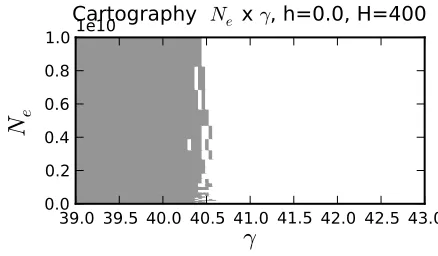
We plot on Figure S1 the Boolean test

(

Q

)

> ǫ

for different values of

N

e

and

γ

for

h

= 0

.

We can see on those plots that the matrix instability does depend on

γ

but not on the

population size. For all the population sizes, the default implementation becomes unstable

(19)

39.0 39.5 40.0 40.5 41.0 41.5 42.0 42.5 43.0

γ

0.0 0.2 0.4 0.6 0.8 1.0

N

e

1e10

Cartography Ne x γ, h=0.0, H=400

Figure S1: One example cartography of the parameter combination that require higher

precision for

ǫ

= 10

−5

_{. We plot the result of the Boolean operation test}

₍

_Q

₍

_{H, h, γ, N}

e

)

≤

ǫ

The legend is True for gray and white for False. We fix

H

= 400

and we plot

N

e

versus

γ

.

for

γ

&

40 .

To conclude, we use one existing method to exponentiate the matrix (Padé) and

imple-mented one more method, with the possibility of increasing the double precision. Which

method to use depends on the type of dataset and the parameter range one needs to

ex-plore. For high values of

γ

, if there are many time intervals, a method based on the spectral

decomposition would be faster, otherwise the Padé approximation works well.

S1.3

Choice of grids

We investigated several grids inspired by Gutenkunst et al. (2009). No matter the

parame-ters, to compute the likelihood we need to approximate the transition probabilities between

the original frequency of the

A

allele,

1

2Ne

, and another frequency between

0 and

1 . Although

we could extrapolate, we instead use grids that all include the point

1 2Ne

.

The first is a uniform grid with a point added at

1

2Ne

. We call this grid the “uniform

grid”. Then we investigate a quadratic grid and an exponential grid. The last two grids

were chosen so that, as opposed to the uniform grid, the distance between adjacent points

changes smoothly.