| MULTIPARENTAL POPULATIONS
A Random-Model Approach to QTL Mapping in
Multiparent Advanced Generation Intercross
(MAGIC) Populations
Julong Wei*,†and Shizhong Xu*,1
*Department of Botany and Plant Sciences, University of California, Riverside, California 92521, and†College of Animal Science and Technology, China Agricultural University, Beijing 100193, China
ABSTRACTMost standard QTL mapping procedures apply to populations derived from the cross of two parents. QTL detected from such biparental populations are rarely relevant to breeding programs because of the narrow genetic basis: only two alleles are involved per locus. To improve the generality and applicability of mapping results, QTL should be detected using populations initiated from multiple parents, such as the multiparent advanced generation intercross (MAGIC) populations. The greatest challenges of QTL mapping in MAGIC populations come from multiple founder alleles and control of the genetic background information. We developed a random-model methodology by treating the founder effects of each locus as random effects following a normal distribution with a locus-specific variance. We alsofit a polygenic effect to the model to control the genetic background. To improve the statistical power for a scanned marker, we release the marker effect absorbed by the polygene back to the model. In contrast to the fixed-model approach, we estimate and test the variance of each locus and scan the entire genome one locus at a time using likelihood-ratio test statistics. Simulation studies showed that this method can increase statistical power and reduce type I error compared with composite interval mapping (CIM) and multiparent whole-genome average interval mapping (MPWGAIM). We demonstrated the method using a publicArabidopsis thalianaMAGIC population and a mouse MAGIC population.
KEYWORDS best linear unbiased prediction; empirical Bayes; mixed model; polygene; restricted maximum likelihood; multiparental populations; Multiparent Advanced Generation Inter-Cross (MAGIC); MPP
T
HERE is an urgent need to develop and study multiparent advanced generation intercross (MAGIC) populations (Rakshitet al.2012). Along with nested association mapping populations (Yuet al.2008), the MAGIC population is called a second-generation mapping resource(Rakshitet al.2012). Using MAGIC populations to perform QTL mapping was first proposed for mice by Threadgillet al.(2002). Such a population is called theCollaborative Cross(CC) population (Churchill et al.2004; Collaborative Cross Consortium 2012). Simulation studies showed that an eight-parent CC population with 1000 progenies is capable of increasing mapping resolution to the sub-centimorgan range (Valdaret al.2006). MAGIC populations inDrosophila melanogaster
are calledDrosophila Synthetic Population Resources(DSPR) (MacDonald and Long 2007; Kinget al.2012a,et al.b). A review of MAGIC populations in crops can be found in Huang et al. (2015). The first plant MAGIC population was developed in Arabidopsis thaliana by Kover et al.
(2009). The population will be described later. Subse-quently, MAGIC populations have been developed in wheat (Huanget al.2012; Mackayet al.2014), rice (Bandilloet al.
2013), and other crop species (Gaur et al. 2012; Pascual
et al. 2015; Sannemann et al. 2015). One key difference between MAGIC populations and other multiparent popu-lations is that all MAGIC lines have experienced multiple generations of inbreeding and thus all are inbred lines. As a result, they are also considered genetic reference popu-lations whose particular genome arrangement can be replicated indefinitely. MAGIC populations in plants un-doubtedly will become more popular in the future of plant genetics and breeding (Varshney and Dubey 2009; Rakshit
Copyright © 2016 by the Genetics Society of America doi: 10.1534/genetics.115.179945
Manuscript received June 26, 2015; accepted for publication December 15, 2015; published Early Online December 29, 2015.
Supporting information is available online at www.genetics.org/lookup/suppl/ doi:10.1534/genetics.115.179945/-/DC1
et al.2012; Huanget al.2015), which calls attention to the need for improvements in statistical methods to analyze and interpret data derived from these populations. A recent call for papers on QTL mapping in MAGIC populations by
GENETICS and G3(http://www.genetics.org/) further in-dicates the urgent need for new technologies in MAGIC population QTL mapping.
Current methods of QTL mapping for MAGIC populations are adopted primarily from methods used in biparental pop-ulations. For example, composite interval mapping (CIM) (Zeng 1994), originally developed for biparental popula-tions, has been used in QTL mapping for MAGIC populations to control genomic background. Other methods and programs of QTL mapping in MAGIC populations include MCQTL (Jourjon
et al.2005), R/qtl (Bromanet al.2003), R happy (Mottet al.
2000), and R/mpMap (Huang and George 2011), most of which have an option to perform CIM. However, there is an intrinsic limitation in cofactor selection, which is more problematic in MAGIC populations than in biparental populations. In an eight-parent-initiated MAGIC population, each marker has 821 = 7 founder effects to estimate. The total number of effects will soon saturate the linear model as the number of cofactors in-creases. For example, a MAGIC population of size 500 will allow only fewer than 500/771 cofactors to be included in the model. When the number of cofactors is small, the CIM procedure is sensitive to the selection of cofactors. Ideally, a model should include all markers in a single model. However, when the marker density is high, genome scanning (a single-QTL model) provides a better alternative method for single-QTL map-ping, but the cofactors should be replaced by a polygenic effect, as done in genome-wide association studies (GWAS) (Yuet al.
2006). We recently developed a QTL mapping procedure by fitting a polygene using a marker-inferred relationship matrix (replacing cofactors) and demonstrated the robustness of the method (Xu 2013b).
Recently, Gattiet al.(2014) developed a mixed model for QTL mapping in Diversity Outbred (DO) mice by treating the effects of scanned markers asfixed and a polygenic effect as random. The polygenic effect essentially replaced cofactors to control the genetic background. The method tends to have a low power because part of the effect of the marker currently scanned is absorbed by the polygene. Our simulation studies showed that dramatic improvement can be achieved in terms of resolution and statistical power of mapped QTL if the effect of the current QTL captured by the polygene is taken into account. Verbyla et al. (2014) developed a multiple-QTL model for QTL mapping in MAGIC populations. The method is calledmultiparent whole-genome QTL analysis
(MPWGAIM), and several steps are involved in selecting markers for inclusion in the model. First, a polygenic base model is implemented to detect the whole-genome effect on the traits of interest. If the polygenic variance is signifi -cantly larger than zero, then markers are subject to selection under a random-model approach;i.e., the founder allelic ef-fects of a marker are treated as random efef-fects, and the var-iance of those founder effects is estimated and the marker is
then selected if the variance is sufficiently large. Thefinal model will include all markers selected (forward selection). This is a variable-selection approach and may be costly if the number of markers and the number of QTL found are large. We will treat this model as the“gold standard”for simulation and comparison. Another recent study of QTL mapping in MAGIC populations is the Bayesian modeling of haplotype effects (Zhang et al. 2014), where the founder haplotype effects are estimated via Markov chain Monte Carlo (MCMC) sampling or importance sampling (IS). One important fea-ture of the Bayesian method is the ability to handle uncer-tainty of the founder allelic inheritance. The only concern with the Bayesian method is the high computational cost when the sample size and the number of markers are very large because Monte Carlo sampling is involved. It is recom-mended to use the Bayesian method tofine-tune the model after markers are selected using some simple methods such as interval mapping (IM) and CIM.
In this study, we extended the mixed-model methodology of QTL mapping in MAGIC populations byfitting a polygenic effect as random and a scanned marker effect either asfixed or random. Furthermore, we released the polygenic counterpart of a scanned marker effect back to the model to avoid competition between the marker effect and its polygenic counterpart. This improved mixed-model methodology has significantly improved the statistical power of QTL detection. We used a CC mouse population (Collaborative Cross Consortium 2012) to perform simulations to examine the properties of the new methods (there are no phenotypic values available for the CC mouse population). TheArabidopsisMAGIC population of Koveret al.
(2009) and the pre-CC mouse population of Rutledge et al.
(2014) were reanalyzed using the new methods to demonstrate the differences between the new and existing methods.
Materials and Methods
MAGIC populations
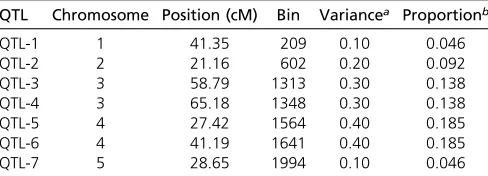
Three MAGIC populations were used in this study to demon-strate the new methods of QTL mapping, two populations in mice and one inA. thaliana. Thefirst MAGIC population in mice does not have phenotypes available on the website (http://www.csbio.unc.edu/CCstatus) and was used only Table 1 Information for the seven simulated QTL using genotypes of thefirst MAGIC population of mice
QTL Chromosome Position (cM) Bin Variancea Proportionb
QTL-1 1 41.35 209 0.10 0.046
QTL-2 2 21.16 602 0.20 0.092
QTL-3 3 58.79 1313 0.30 0.138
QTL-4 3 65.18 1348 0.30 0.138
QTL-5 4 27.42 1564 0.40 0.185
QTL-6 4 41.19 1641 0.40 0.185
QTL-7 5 28.65 1994 0.10 0.046
aVariance of a QTL, which is defined asvarðZ
kgkÞ, and the variance is taken across all individuals in the MAGIC population.
for simulation studies. The second MAGIC population of mice has both genotype and phenotype information and was used as a real application example. The MAGIC population in
A. thalianaalso has both genotype and phenotype information and was reanalyzed to compare the results of the different methods.
First MAGIC population of mice:This MAGIC population is called theCC population(Churchillet al.2004). The genotype data were published by the Collaborative Cross Consortium (2012). No phenotype information is available in the 458 CC mice, and thus the data were used only for simulation study. The CC population is an eight-parent MAGIC population de-rived from a funnel mating design. We downloaded the re-combination breakpoint data of 19 autosomes from 458 CC mice posted on the University of North Carolina (UNC) Sys-tem Genetics website (http://www.csbio.unc.edu/CCstatus). Using the breakpoint information, we inferred 6683 bins (in-tact chromosome segments). A bin is defined as a segment that contains no breakpoints across all lines within the seg-ment. Within a bin, all markers segregate in exactly the same pattern across lines (perfect LD). Therefore, a single marker can represent the whole bin. For detailed information on bin data analysis, see Xu (2013a). The bin data are available in Supporting Information,File S1.
Second MAGIC population of mice: The second MAGIC population was derived from the same eight parents as the first CC population, but the CC mice were not fully inbred, and therefore, the population is called thepre-CC population. The data were obtained from Rutledgeet al.(2014) and consist of 151 individuals. This data set includes 27,039 SNPs evenly distributed among the 20 chromosomes (including the X
chromosome). Probabilities of the parental origins of the SNPs were calculated using the HAPPY program based on the hidden Markov model (Mottet al.2000). In the original study of this population, the authors focused on two traits associated with severe asthma and decrements in lung func-tion, including airway polymorphonuclear neutrophil (PMN) recruitment and the concentration of CXCL1 in lung lavage fluid. Here we reanalyzed thefirst trait, PMN.
MAGIC population of Arabidopsis:The MAGIC population of A. thaliana (Kover et al. 2009) consists of 527 lines
descended from a heterogeneous stock of 19 intermated par-ents. These lines and the 19 founders were genotyped with 1260 SNP markers [minor allele frequency (MAF).5%] and phenotyped for two development-related traits, the number of days between bolting andflowering (DBF) and growth rate (GR), where GR was measured as the residual of regression by fitting the number of leaves to the number of days to germination. The 527 lines were derived from the 19 founder accessions of A. thaliana, intermating for four generations, and then inbreeding for six additional generations, forming nearly homozygous lines. The authors further updated the database after the initial publication. We downloaded the updated genotypes and phenotypes from http://mus.well. ox.ac.uk/magic/. There were only 426 lines having both the genotype and phenotype information. In this analysis, we included the 426 lines and 1254 markers distributed among five chromosomes (total length of the genome is 118 Mb). The founder strain probabilities for all loci were calculated using the HAPPY program. We analyzed both DBF and GR.
Statistical methods
Polygenic model:The polygenic model is the null model used to scan the entire genome for QTL identification. We now use an eight-parent MAGIC population as an example to demon-strate the model. The method holds for anyp-parent MAGIC populations. Letybe ann31 vector of phenotypic values for
nindividuals. DefineZkas ann38 matrix of founder allele
inheritance indicators for locusk. Thejth row of matrixZkis
defined as a 138 vector. If this individual is a heterozygote carrying thefirst and second founder alleles, then we define
Zjk¼ ½1 1 0 0 0 0 0 0
If the individual is a homozygote inheriting both alleles from thefifth founder, thenZjkis defined as
Zjk¼ ½0 0 0 0 2 0 0 0
The general rule for definingZjkis that there are at most two
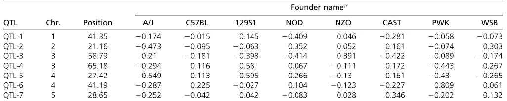
nonzero elements, and the sum of all eight elements equals 2. We then define the following polygenic model, which is the null model used to test significance of an individual marker: y¼Xbþjþe (1) Table 2 Founder effects for the seven simulated QTL using genotypes of thefirst MAGIC population of mice
Founder namea
QTL Chr. Position A/J C57BL 129S1 NOD NZO CAST PWK WSB
QTL-1 1 41.35 20.174 20.015 0.145 20.409 0.046 20.281 20.058 20.073
QTL-2 2 21.16 20.473 20.095 20.063 0.352 0.052 0.161 20.074 0.303
QTL-3 3 58.79 0.21 20.181 20.398 20.414 0.391 20.422 20.089 20.174
QTL-4 3 65.18 20.294 0.116 0.58 0.067 20.111 0.172 20.443 0.267
QTL-5 4 27.42 0.549 0.113 0.595 0.266 20.13 0.161 20.43 20.265
QTL-6 4 41.19 20.287 0.225 20.027 0.104 20.123 20.227 0.809 0.061
QTL-7 5 28.65 20.252 20.042 0.042 20.083 0.028 0.346 20.202 0.132
whereXis ann3rdesign matrix forrfixed effects;bis an
r31 vector for therfixed effects;jis ann31 vector of polygenic effects with an assumed multivariate normal distribution jNð0;Kf2Þ, where K is a marker-derived kinship matrix and f2 is a polygenic variance; and eNð0;Is2Þ is a vector of residual errors with an
un-known error variances2. The marker inferred kinship
ma-trix is defined as
K¼1
d Xm
k¼1
ZkZTk (2)
whered¼ ð1=nÞtrðPkm¼1ZkZTkÞis a normalization factor. The
expectation of yis EðyÞ ¼Xb, and the variance-covariance matrix is
varðyÞ ¼Kf2þIs2¼ ðKlþIÞs2¼Hs2 (3)
wherel¼f2=s2is the variance ratio, andH¼KlþI. After
absorbing b and s2, the restricted maximum likelihood is
only a function ofl, which is
LðlÞ ¼ 21 2lnjHj2
1 2lnjX
TH21Xj2n2r
2 lnðy
TPyÞ (4)
where
P¼H212H21XðXTH21XÞ21XTH21 (5)
The restricted maximum likelihood solution oflwas obtained by maximizing the preceding likelihood function using the Newton iteration algorithm. The eigen-decomposition algo-rithm proposed by Kanget al.(2008) was used to evaluate the likelihood function for fast computation. The estimated variance ratio is denoted by bland will be used as a known constant in the genomic scanning model that follows.File S2
describes the method of estimatinglalong with the effect of the marker scanned, the so-called exact method (Zhou and Stephens 2012).
Fixed model:To test the significance of thekth marker, we first used thefixed-model approach proposed by Gattiet al.
(2014). The model is
y¼XbþZkgkþjþe (6)
where Zk is the allelic inheritance matrix for marker k, as
defined earlier, and
gk¼ ½g1k g2k g3k g4k g5k g6k g7k g8kT (7)
is an 831 vector for the eight founder allelic effects. Under this model, thegkvector is assumed to befixed effects. The
model is in fact a mixed model because it contains bothfixed and random effects. We call it thefixed modelbecause later on we will treatgkas random effects. Under thefixed model, we
can only estimate and test seven (8–1 = 7) effects by de-leting the last founder allele from the model. The maximum-likelihood method was used to estimate gk, and the result
turned out to be identical to the weighted-least-squares esti-mate after premultiplying all variables (y,X, andZk) by the
eigenvectors of theKmatrix and the weight for thejth indi-vidual beingWj¼1=ðdjlbþ1Þ, wheredjis thejth eigenvalue
of the K matrix (Xu 2013b). Note that blis the estimated variance ratio under the polygenic model, as described ear-lier. This method is called theapproximate method(Zhou and Stephens 2012). The likelihood-ratio test was used as the test statistic and is defined as
Gk¼ 22
L0eb;se2
2L1bb;bgk;bs2
(8)
whereL0is the log likelihood function under the null model
(gk = 0), andL1 is the log likelihood function under the
alternative model. Note that the estimated bands2under
the two models are different. The P-value was calculated from the chi-square distribution with seven degrees of free-dom. This method is called FIXED-Awhen compared with other methods.
Recall thatZkcontributes to the calculation of the
kin-ship matrix K, as shown in equation 2. Although not ex-plicitly estimated in the polygene, the effect of marker k
has a polygenic counterpart that may compete with the estimatedgk when markerkis scanned. Letbjk¼Zkbakbe
the estimated polygenic effect contributed by marker k, and bak is the estimated effect for this marker under the
polygenic model. We can release this effect from the poly-gene back to the model to avoid this competition. The re-vised model is
y¼XbþZkgkþj2bjkþe (9)
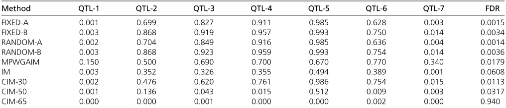
Table 3 Statistical powers for the seven simulated QTL and FDR drawn from 1000 replicated simulation experiments
Method QTL-1 QTL-2 QTL-3 QTL-4 QTL-5 QTL-6 QTL-7 FDR
FIXED-A 0.001 0.699 0.827 0.911 0.985 0.628 0.003 0.0015
FIXED-B 0.003 0.868 0.919 0.957 0.993 0.750 0.014 0.0034
RANDOM-A 0.002 0.704 0.849 0.916 0.985 0.636 0.004 0.0014
RANDOM-B 0.003 0.868 0.923 0.959 0.993 0.754 0.014 0.0036
MPWGAIM 0.150 0.500 0.690 0.700 0.670 0.770 0.340 0.0179
IM 0.003 0.352 0.326 0.355 0.494 0.389 0.001 0.0608
CIM-30 0.002 0.476 0.620 0.761 0.986 0.754 0.015 0.0113
CIM-50 0.001 0.136 0.043 0.015 0.512 0.009 0.003 0.0317
Rearranging this equation leads to
yþbjk¼XbþZkgkþjþe (10)
Further definingyk¼yþbjk, we now have a new model yk¼XbþZkgkþjþe (11)
which is the same as equation 6 except that the y vector changes every time a marker is scanned. Note that bjk, the
polygenic component from markerk, is calculated only once under the null model. Therefore, this revised method does not present much additional computational burden. The method to obtainbjkis called thebest linear unbiased predic-tion(BLUP) and is described inFile S2. This revised method is calledFIXED-Bwhen compared with other methods.
Random model: The fixed-model approach may not be stable when the number of founders is large (Gattiet al.
2014), and the design matrix Zk may have variable
ranks across different markers. Under the null model, the likelihood-ratio test statistic follows a chi-square dis-tribution with degrees of freedom depending on the num-ber of founders. We propose to treat the eight founder effects as random variables following a normal distribu-tion with mean zero and a common variance. Although it is still a mixed model, we call it arandom modelto distin-guish it from thefixed model described earlier. The linear model remains the same as equation 6, butgkNð0;I8f2kÞ
is assumed, where f2k is a locus-specific variance. The expectation of y remains EðyÞ ¼Xb, and the variance-covariance matrix is
varðyÞ ¼ZkZTkf2kþKf2þIs2¼ZkZTkfk2þ ðKlþIÞs2 ¼ZkZTkf2kþHs2
(12)
wherelinHis replaced by the estimated value under the poly-genic model. A restricted-maximum-likelihood (REML) estimate off2k is obtained by maximizing the restricted likelihood func-tion. Woodbury matrix identities (Golub and Van Loan 1996) are applied along with the eigen-decomposition to ease the computational burden (File S2). The null hypothesis for marker
kisf2k¼0, which is tested using the likelihood-ratio test
Gk¼ 22
L0eb;se2
2L1bb;fb 2 k;bs
2
(13)
Under the null model, this test statistic follows approximately a mixture ofx20andx
2
1distributions with an equal weight
(Chernoff 1954; Visscher 2006). This method is called
RANDOM-Awhen compared with other methods.
We also developed a revised version of the random model by avoiding competition between the current marker scanned and its polygenic counterpart using model 11 as we did for the fixed model. This revised random model is calledRANDOM-B
to distinguish it from other methods.
Multiparent whole-genome average interval mapping (MPWGAIM): Here we also performed the analysis using the MPWGAIM approach proposed by Verbylaet al.(2014) for comparison using their R package mpwgaim. In the mpwgaim package, only detected markers are reported with-out test statistics attached. For comparison with our methods, we calculated the Wald test statistics of detected markers based on their estimated effects and variances and then obtained the P-value from the chi-square distribution with 821 = 7 degrees of freedom. For the simulated data anal-ysis, we also applied the MPWGAIM method. The empirical critical value for hypothesis test was inferred from multiple (1000) simulations under the null model. The 95th percentile
of the highest Wald test from each of the multiple simulations was chosen as the empirical critical value. The P-value was transformed by2log10and used to determine whether or not
a marker exceeds the empirical critical value.
IM and CIM:IM (Lander and Botstein 1989) and CIM (Zeng 1994) also were used to analyze the data to compare the results with the new methods. These two methods are called
method was implemented in the HAPPY program (Mottet al.
2000). The CIM method was implemented using our own R program. For the CIM-xmethod, the number of cofactorsx
was set at the following levels for thefirst MAGIC population of mice: 65, 50, and 30. For a sample size of 458, the maxi-mum number of cofactors cannot be higher than 458/765; otherwise, there will not be any degrees of freedom left to estimate the residual error variance. For the second MAGIC population of mice (the pre-CC population), the number of cofactors was set at 20, 10, and 5. The population size is 151, and thus the number of cofactors cannot be higher than 151/720. For theArabidopsispopulation, the number of cofactors was set at 20, 15, and 10. The maximum number of
possible cofactors cannot be greater than 428/1823. The likelihood-ratio test statistic also was used for the IM and CIM methods.
P-value and permutation: We now have a total of seven methods to compare: FIXED-A, MPWGAIM, IM, and CIM are existing methods, and FIXED-B, RANDOM-A, and RANDOM-B are new methods proposed in this study. The P-value of a marker was calculated from the central chi-square distribu-tion with 821 = 7 degrees of freedom for the two mouse populations and 19 21 = 18 degrees of freedom for the
RANDOM-B methods, theP-value for each marker was cal-culated from a mixture of two chi-square distributions, denoted by 1
2x 2 0þ12x
2
1, where x20 is just a fixed number of
0 (Chernoff 1954; Visscher 2006). LetPkbe theP-value for
markerk, it was calculated using
Pk¼
1 Gk¼0
1 2Pr
x21.Gk
Gk.0
(14)
whereGkis the likelihood-ratio test statistic calculated using
equation 13, andx21is a chi-square variable with one degree
of freedom. In the real data analysis, we permuted the data 1000 times to generate a null distribution of the test statistics [2log10ðPÞ]. From this null distribution, we determined the
95% quantile and used it as an empirical critical value of a test statistic. A marker with the test statistic [2log10ðPÞ]
so that the polygenic covariance structure remains the same as that in the original data set. This kind of permutation will not destroy the polygenic variance (Cheng and Palmer 2013). Note that permutation was used only in real data analysis to generate empirical critical values for significance tests. In power calculation of the simulated data analysis, empirical critical values were generated from multiple simu-lations under the null model.
Simulation experiment
The simulation experiment was conducted based on the genotypic data of the first MAGIC population of mice (the CC population). As a result, the sample size wasfixed at 458. We used genotypes of thefirstfive chromosomes as the true genotypes to conduct the simulation experiment. The five chromosomes contain 490, 503, 428,423, and 406 bins, re-spectively, leading to a total of 2250 bins. The design of the simulated QTL mimicked closely that of Verbylaet al.(2014). We simulated a total of seven QTL distributed on the five chromosomes. Information about the seven simulated QTL is shown in Table 1. The simulated allelic effects of the eight founders are given in Table 2. The polygenic and residual error variances were set at f2= 0.5 ands2= 0.5,
respec-tively. The seven QTL collectively have a total variance of 1.1752, which is partitioned into the sum of variances for all seven QTL (1.80) plus twice the sum of all covariances 20.6248 (1.80 20.6248 = 1.1752). The total phenotypic variance is 1.1752 + 0.5 + 0.5 = 2.1752. Therefore, the proportion contributed to the phenotypic variance by all seven QTL is 1.1752/2.1752 = 0.5403. The proportion of the polygenic variance contributed to the phenotypic vari-ance is 0.5/2.1752 = 0.2298. The total genetic contribution (QTL + polygene) is 0.5403 + 0.2298 = 0.7701. QTL-1 and -7 are small in terms of the proportions contributed to the trait phenotypic variance. The remaining four QTL are rela-tively large.
Under the preceding parameter setups, we generated 1000 independent data sets to evaluate the empirical powers under a 0.05 type I error. We also generated 1000 additional data sets under the null model (no QTL were simulated but the poly-gene). Results of the data analysis from the null model were used to generate the empirical distribution of the test statistics [2log10ðPÞ] and draw the empirical thresholds of the test
statistics for hypothesis tests. The statistical powers from the 1000 replicated simulation experiments were reported by comparing the results with the empirically drawn thresholds
of the test statistics. For each simulated QTL, a65-cM window around the true position was reserved for power calculation, as done by Verbyla et al.(2014). If any bin within this window was detected, the QTL covered by this window was claimed to be detected. Any detected bins beyond this window were counted as false positives. All seven methods mentioned earlier were used to analyze the simulated data. The empirical powers were compared for the seven methods.
Data availability
The new methods of QTL mapping for MAGIC populations were implemented in an R package calledMagicQTL, which is provided in the Supporting Information and downloadable from the journal article website (seeFile S3for the R package andFile S4for the user instruction of the R package). R codes for data simulation, data preparation, and data analysis are downloadable fromhttps://github.com/JulongWei/MagicQTL. This website also provides the R code for calling the MPWGAIM package.
Results
Simulation studies
Statistical powers and false discovery rate (FDR): The empirical statistical powers drawn from 1000 replicated sim-ulations are given in Table 3. In general, the RANDOM-A and RANDOM-B methods have slightly higher powers than the FIXED-A and FIXED-B methods for the five large simulated QTL. The FIXED-B and RANDOM-B methods have substan-tially higher powers than the FIXED-A and RANDOM-A meth-ods. The MPWGAIM method has lower power for the first four large QTL (QTL-2 to QTL-5) than that of the FIXED-A, FIXED-B, RANDOM-A, and RANDOM-B methods. The MPWGAIM method has an advantage over the other methods for detecting the following three QTL: QTL-1, QTL-6, and QTL-7. Except for the MPWGAIM method, no methods have sufficient power to detect the two small QTL (QTL-1 and QTL-7). Overall, the new methods (i.e., FIXED-B, RANDOM-A, and RANDOM-B) are more powerful than the existing methods (i.e., FIXED-A, MPWGAIM, IM, and CIM) for large QTL.
We also compared the FDR for the seven methods (see the last column of Table 3). Here we define the FDR as the proportion of detected QTL that are not true (65.00 cM away from a simulated QTL). Clearly, the FIXED-A, FIXED-B, RANDOM-A, and RANDOM-B methods achieve better control of the FDR than the MPWGAIM method, which, in general, is better than the IM and CIM methods.
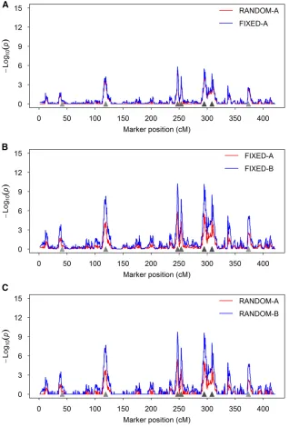
Behaviors of the methods: Wefirst demonstrate the differ-ence between the random model and thefixed model in terms of the test statistic expressed as2log10ðPÞof scanned markers
using a single simulated data set (Figure 1). Figure 1A shows the difference between the RANDOM-A and FIXED-A meth-ods. Clearly, the test statistic of the FIXED-A method is Table 4 Estimated variance components and heritability of two
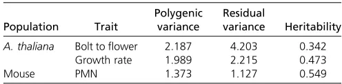
traits in the A. thalianapopulation and one trait in the mouse population Population Trait Polygenic variance Residual variance Heritability
A. thaliana Bolt toflower 2.187 4.203 0.342
Growth rate 1.989 2.215 0.473
slightly higher than that of the RANDOM-A method. We also noticed that the 2log10ðPÞ statistic for the RANDOM-A
method is very close to zero in regions where no QTL was simulated. This demonstrates the shrinkage property of the random method. In either case, the test-statistic profiles show clear peaks at positions where simulated QTL reside, and the heights of the peaks are proportional to the sizes of the sim-ulated QTL. Figure 1B compares the FIXED-A and FIXED-B methods, where the2log10ðPÞprofile of the FIXED-B method
shows higher peaks than the FIXED-A method. This implies that the FIXED-B method may have a higher power than the FIXED-A method. Figure 1C compares the RANDOM-A and RANDOM-B methods. This also implies that releasing the polygenic counterpart of a marker back to the model may help to increase the power of detecting this marker. These types of behaviors are expected to be observed in data anal-yses of real experiments.
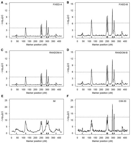
Average test-statistic profiles:We replicated the simulation experiment 1000 times under both the null model (without QTL effects) and the alternative model (with simulated QTL). The average test-statistic profiles [2log10ðPÞ] over the 1000
replicates and the 95% threshold values are illustrated in Figure 2. Comparing thefixed models (Figure 2, A and B) with the random models (Figure 2, C and D), we found that the test statistics are slightly higher for thefixed models than for the random models, but the former are also associated with higher threshold values in the test statistics. Comparing -A models (Figure 2, A and C) with -B models (Figure 2, B and D), the latter have higher peaks at positions where simulated QTL reside. For the four models, peaks corresponding to the five large QTL are higher than the threshold values, but peaks corresponding to the two small QTL are below the thresholds. The peaks for the second QTL barely touch the thresholds for
-A models (Figure 2, A and C), indicating that the modified models (releasing the polygenic effect back to the model) help to boost the power. None of the peaks in IM reaches the threshold value (Figure 2E). CIM with 30 cofactors only detected four of the five large QTL (Figure 2F). When we increased the number of cofactors to 50 and 65, the CIM method behaved very badly (Figure S1). For the MPWGAIM method, owing to the lack of the test statistics in the package, we only reported the power and FDR.
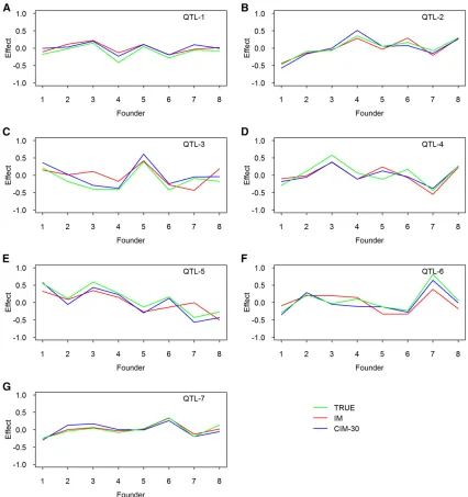
Average estimated founder effects: We also estimated the founder effects for the seven simulated QTL based on all simulations, and they are illustrated in Figure 3 for thefixed and random models and in Figure 4 for the IM and CIM procedures. The true effects also were plotted along with the estimated effects. All methods provided good estimates of the founder effects. The random models tend to shrink the estimated effects toward zero when the simulated QTL sizes are small (Figure 3, A and G). Although the IM and CIM methods are not as good as the other methods in terms of statistical power, both gave very good estimated founder ef-fects.Figure S2shows the average estimated effects of the founders when 50 and 65 markers were used as cofactors for the CIM method.
Results of experimental data analyses: MAGIC population in A. thaliana:Under the polygenic model, we estimated the variance and heritability for each of the two traits, the days between bolting andflowering (DBF), and the growth rate (GR). The results are shown in Table 4. The heritability of the two traits is 0.342 and 0.473, respectively. The variance ratios for DBF and GR are blDBF¼fb
2
=bs2¼0:5203 and
b lGR¼bf
2
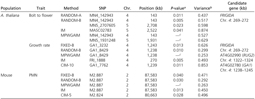
=sb2¼0:8980, respectively, which were used as known values and incorporated into the covariance structures Table 5 Significant SNPs associated with two traits in theA. thalianapopulation and one trait in the mouse population
Population Trait Method SNP Chr. Position (kb) P-valuea Varianceb
Candidate gene (kb)
A. thaliana Bolt toflower RANDOM-A MN4_142943 4 143 0.011 0.437 FRIGIDA
RANDOM-B MN4_142943 4 143 0.005 0.517 Chr.4: 269–272
MN5_2707605 5 2,708 0.023 0.598
IM MASC02783 5 2,522 0.041 0.874
MPWGAIM MN4_142943 4 143 —c 0.527
MN5_1931248 5 1,931 —c 0.629
Growth rate FIXED-B GA1_3232 4 1,243 0.013 0.626 FRIGIDA
RANDOM-B GA1_8429 4 1,238 0.010 0.299 Chr.4: 269–272
MPWGAIM GA1_8429 4 1,238 —c 0.253 AT4G02990 (RUG2)
IM FRI_1888 4 270 0.005 0.493 Chr.4: 1322–1324
CIM-10 GA1_7762 4 1,239 0.011 0.853 AT4G02780 (GA1)
Chr.4: 1238–1245
Mouse PMN FIXED-B M2.887 2 87,583 0.040 0.471
RANDOM-B M2.887 2 87,583 0.030 0.292
MPWGAIM M2.887 2 87,583 —c 0.263
IM M2.887 2 87,583 0.013 0.450
CIM-5 M2.824 2 80,663 0.028 0.496
aP-value was obtained from a permutation test.
for genomic scanning of all markers. Figure 5 illustrates the test-statistic profiles [2log10ðPÞ] along with the 95%
thresh-olds generated from 1000 permuted samples for DBF. Markers with test-statistic values greater than the thresholds were claimed to be statistically significant. There are two peaks standing out on chromosomes4and5, respectively, for all methods except CIM-10. These two regions also showed up in the original analysis of Koveret al. (2009). However, the only method that detected both peaks is RANDOM-B, implying that this method may be the most powerful method. The de-tected QTL on chromosome4is located near a known gene calledFRIGIDA. No related genes were found near the detected
QTL on chromosome5. The MPWGAIM method also detected the two QTL in the same regions (Table 5). In addition, the MPWGAIM method detected three more QTL, one on chromosome 1(PERL0236029) and two on chromosome3
(MASC00175 and MN3_22843506). Figure S3 (A and B) shows the results of this data analysis using the CIM method when 15 and 20 markers were used as cofactors.
all six methods. Except the FIXED-A and RANDOM-A meth-ods, all other methods have detected the peak as statistically significant. We list the SNPs exceeding the threshold values in Table 5. Three candidate genes are found in this area (about 6200 kb around the detected marker), FRIGIDA, AT4G02990 (RUG2), and AT4G02780 (GA1). Thefirst candi-date gene (FRIGIDA) is known to affectflowering time. This gene is also related to growth rate in the original study (Kover
et al.2009), where it was pointed out that this gene not only plays an important role in plan reproduction but also is a major determinant of the plant developmental process. The second candidate gene (RUG2) is important for leaf
development inA. thaliana, and its loss of function leads to a pleiotropic phenotype, including leaf variegation, reduced growth, and perturbed mitochondrial and chloroplastic gene expression and development (Quesadaet al.2011). The third candidate gene (GA1) codes for the enzymeent-kaurene syn-thase A. InGA1mutants, the gibberellin biosynthesis path-way is inactivated. As a result, these mutants are deficient in bioactive Gas (Sun and Kamiya 1994). Some additional markers are detected by the IM and MPWGAIM methods, and they are listed inTable S1. The markers on chromosomes
methods also show some bumps in regions near the addi-tional markers detected by the IM and MPWGAIM methods. These regions (about6200 kb around the peaked markers) harbored several candidate genes, which are not related to GR in terms of gene function.Figure S3(C and D) shows the results when 15 and 20 markers were used as cofactors for the CIM method.
Pre-CC population of mice:We analyzed a trait named PMN from this population. The phenotypic values were log trans-formed prior to the analysis, as done in the original study. We estimated the genetic variance and heritability of the trait, which are presented in Table 3. The trait is highly heritable, with a heritability of 0.55. The variance ratio is b
l¼fb2=bs2¼1:373=1:127¼1:2183, which was used along
with the kinship matrix to control the polygenic effect in QTL mapping. We scanned the entire genome using all seven methods. The test-statistic profiles are illustrated in Figure 7. Except for the FIXED-A and RANDOM-A methods, all other methods detected a marker on chromosome2(Table 5). This marker also was detected by Rutledge et al. (2014) in the original study. They found a candidate gene (Dpn1) near this marker. No other candidate genes were found in the neigh-borhood of this marker.Figure S3(E and F) shows the results when 10 and 20 markers were used as cofactors for the CIM method.
Discussion
A key difference between QTL mapping in MAGIC and bi-parental populations is the difference in the number of effects to be estimated and tested per locus. Under thefixed-model framework, for an eight-parent MAGIC population, the num-ber of effects per locus is 821 = 7, while it is always 221 = 1 for a biparental population. Under the null model, the likeli-hood-ratio text follows a chi-square distribution with 7 de-grees of freedom. In ap-parent MAGIC population,p21 is the degrees of freedom. Whenpis large, this test is not con-venient and sometimes can be unstable (Gatti et al.2014). For example, if some founder alleles fail to appear in the progeny for some loci, theZmatrices for these loci will not have the same rank as those loci with full representation of all founders. This variable-rank situation will cause some difficulty in programming. More important, the degree of freedom will vary across loci, so the likelihood-ratio text sta-tistic will not be comparable across loci. We developed a random-model approach to estimate and test the variance
among all founder effects per locus. As a result, we only need to estimate and test a single parameter (the variance) regard-less how large the number of founders is in a MAGIC popu-lation. Simulation studies showed that the random-model approach is slightly more powerful than the fixed-model approach.
Some investigators also considered founder allelic effects as random in MAGIC population QTL mapping (Verbylaet al.
2014; Zhang et al. 2014). The MPWGAIM procedure of Verbylaet al.(2014) assumes that all founder allelic effects of the same locus share a common variance and that this variance varies across loci. A forward variable selection approach was adopted by adding one locus at a time to the model until no further improvement was achieved. For consistency of com-parison, we adopted the critical value generated from the null model, similar to the other methods, to evaluate the power of QTL detection by the MPWGAIM method using the same test criterion. We demonstrated lower powers (for large QTL) and higher FDR for the MPWGAIM method. The MPWGAIM method can be time consuming if the numbers of markers and QTL included in the model are large. Table 6 compares the computational times of our methods with that of the MPWGAIM method under several different scenarios. Clearly, the new genome-scanning approaches proposed in this study are substantially faster than the MPWGAIM method. The Bayesian method of Zhang et al.(2014) also treats founder allelic effects as random, and it is a multiple-QTL model. Because the method is implemented via an MCMC sampling scheme, it is also computationally expen-sive. The authors suggested that the method is better used to fine-tune the results after an initial genome scan of all markers.
When cofactors are replaced by the polygene for back-ground control, there is a potential competition between a currently scanned marker and its counterpart in the polygene, which is detrimental to the power. The competition can be very serious when the number of markers used to calculate the kinship matrix is small, although it may be negligible when a very large number of markers are used to calculate the kinship matrix. To prevent such a competition, we proposed releasing the polygenic component corresponding to the scanned marker back to the model. This has dramatically increased the statistical power of QTL detection. The BLUP estimate of a marker effect in the polygene is calculated only once prior to the marker scanning step, and thus little additional compu-tational cost is present. We could have removed the currently Table 6 Computational performances of different methods with different sample sizes and different numbers of markers
Method Mouse-458-2250a Mouse-458-6683b Mouse-151-27309 Arabidopsis-426-1254
FIXED-A 22 sec 53 sec 1 min 43 sec 23 sec
FIXED-B 41 sec 1 min 44 sec 4 min 25 sec 34 sec
RANDOM-A 36 sec 1 min 42 sec 5 min 21 sec 27 sec
RANDOM-B 55 sec 2 min 31 sec 8 min 10 sec 39 sec
MPWGAIM 32 min 29 sec 2 h 33 min 1h 33 min 11 min 51 sec
scanned marker from the kinship matrix to avoid the com-petition. However, this would substantially increase the computational burden because a new kinship matrix would have to be provided for each marker scanned. Special algorithms, such as the spectrally transformed linear mixed model (FaST-LMM) proposed by Lippertet al.(2011), may be used to ease the computational intensity. However, the fast speed is not achieved without a cost. One has to use markers with a number substantially smaller than the sam-ple size to gain the fast speed. When the number of markers used to construct the kinship matrix is too small, optimal control of the polygene may not be guaranteed (Zhou and Stephens 2012).
The genotype coding system of QTL mapping in MAGIC populations is different from that in biparental populations. We used theZk variable (ann38 matrix) to indicate the
founder allelic inheritances for thekth marker. This variable also was used to calculate the marker-inferred kinship matrix
K. The kinship matrix was eventually rescaled by a normali-zation factor, which is the average of the diagonal elements of the original unnormalized kinship matrix. After normaliza-tion, the diagonal elements of the kinship matrix are all around unity. Such normalization will bring the estimated polygenic variance into the same scale as the residual error variance. Our normalization factor is different from that pro-posed by VanRaden (2008), which is the sum of heterozygos-ity across all loci. The normalization factor only changes the scale of the estimated polygenic variance; it affects neither the hypothesis tests nor the results of QTL mapping. In GWAS, where theZkvariable is simply a vector, Kanget al.
(2008) placed a weight variable for each marker in calculat-ing the kinship matrix to take into account variable informa-tion contents (allele frequencies) across different marker loci. It is not obvious how to evaluate information contents when the genotype indicator variableZkfor each marker is a
ma-trix. In CC and pre-CC mice, all founders contributed equally to the mapping population, and thus, the weight variable can be safely ignored (e.g., taking the default value of 1 from all markers). In the 19-parent MAGIC population ofArabidopsis, where the parental contribution varies across founders, a weighted kinship matrix may be more appropriate. Further study is needed to develop an appropriate weight matrix. Alternatively, the method of Gattiet al.(2014) for calculating the kinship matrix may be adopted here. The relationship between each pair of individuals is a kind of average“scaled similarity”over all loci. In our notation, the relationship be-tween individualsiandj(theith row and thejth column of the kinship matrix) is expressed as
Kij¼
1
m Xm
k¼1
ZT ikZjk
ffiffiffiffiffiffiffiffiffiffiffiffi ZT
ikZik
q ffiffiffiffiffiffiffiffiffiffiffiffi ZT
jkZjk
q (15)
We did not use this kinship matrix because the polygenic counterpart of markerk(used in the FIXED-B and RANDOM-B methods) would be difficult to interpret when thisKmatrix
is used. Furthermore, whether or not such a kinship matrix can adjust unbalanced contributions from different founders is still questionable.
The random-model approach is a kind of Bayesian analysis if the founder effects are considered as parameters and the variance of the founder effects is considered as a prior vari-ance. Because the prior variance is estimated from the data, it is called empirical Bayes(Xu 2007).The random model de-veloped for QTL mapping in MAGIC populations can be used in a number of other situations. The method can be extended to QTL mapping in DO populations, such as the DO popula-tion of mice developed from the same eight parents as the CC mice (Gattiet al.2014).
The random-model approach is computationally more in-tensive than thefixed-model approach, where the QTL effects are treated asfixed effects because it requires estimation of a variance component for each marker scanned. We adopted the eigen-decomposition algorithms for the polygenic (null) model and combined them with the Woodbury matrix identity for estimation of QTL variance. It would not be realistic to perform such a random-model QTL mapping without resort to these special algorithms. There may be room for further improvement in the computational speed. However, we emphasize the concept and the novelty of the method, which are far more important than technical im-provement in computational speed. Finally, all analyses were performed using an R program written by the authors. We developed an R package named MagicQTL, which is provided on the journal website.
Acknowledgments
We thank Arunas P. Verbyla for sharing the mpwgaim program and for the tremendous help in running this program. We also thank Samir N. P. Kelada for providing the pre-CC mouse data. This project was supported by National Science Foundation grant 005400 to S.X. and a China Scholarship Council Award to J.W.
Literature Cited
Bandillo, N., C. Raghavan, P. A. Muyco, M. A. L. Sevilla, I. T. Lobina
et al., 2013 Multi-parent advanced generation inter-cross (MAGIC) populations in rice: progress and potential for genetics research and breeding. Rice 6: 1–15.
Broman, K. W., H. Wu, ´S. Sen, and G. A. Churchill, 2003 R/qtl: QTL mapping in experimental crosses. Bioinformatics 19: 889– 890.
Cheng, R., and A. A. Palmer, 2013 A simulation study of permu-tation, bootstrap, and gene dropping for assessing statistical significance in the case of unequal relatedness. Genetics 193: 1015–1018.
Chernoff, H., 1954 On the distribution of the likelihood ratio. Ann. Math. Statist. 25: 573–578.
Churchill, G. A., D. C. Airey, H. Allayee, J. M. Angel, A. D. Attie
Collaborative Cross Consortium, 2012 The genome architecture of the Collaborative Cross mouse genetic reference population. Genetics 190: 389–401.
Gatti, D. M., K. L. Svenson, A. Shabalin, L.-Y. Wu, W. Valdaret al., 2014 Quantitative trait locus mapping methods for Diversity Outbred mice. G3 4: 1623–1633.
Gaur, P. M., A. K. Jukanti, and R. K. Varshney, 2012 Impact of genomic technologies on chickpea breeding strategies. Agronomy 2: 199–221.
Golub, G. H., and C. F. Van Loan, 1996 Matrix Computations, Ed. 3. Johns Hopkins University Press, Baltimore.
Huang, B. E., and A. W. George, 2011 R/mpMap: a computational platform for the genetic analysis of multiparent recombinant inbred lines. Bioinformatics 27: 727–729.
Huang, B. E., A. W. George, K. L. Forrest, A. Kilian, M. J. Hayden
et al., 2012 A multiparent advanced generation inter‐cross population for genetic analysis in wheat. Plant Biotechnol. J. 10: 826–839.
Huang, B. E., K. L. Verbyla, A. P. Verbyla, C. Raghavan, V. K. Singh
et al., 2015 MAGIC populations in crops: current status and future prospects. Theor. Appl. Genet. 128: 999–1017.
Jourjon, M.-F., S. Jasson, J. Marcel, B. Ngom, and B. Mangin, 2005 MCQTL: multi-allelic QTL mapping in multi-cross de-sign. Bioinformatics 21: 128–130.
Kang, H. M., N. A. Zaitlen, C. M. Wade, A. Kirby, D. Heckerman
et al., 2008 Efficient control of population structure in model organism association mapping. Genetics 178: 1709–1723. King, E. G., S. J. MacDonald, and A. D. Long, 2012a Properties
and power of the DrosophilaSynthetic Population Resource for the routine dissection of complex traits. Genetics 191: 935–949.
King, E. G., C. M. Merkes, C. L. McNeil, S. R. Hoofer, S. Senet al., 2012b Genetic dissection of a model complex trait using the
Drosophila Synthetic Population Resource. Genome Res. 22: 1558–1566.
Kover, P. X., W. Valdar, J. Trakalo, N. Scarcelli, I. M. Ehrenreich
et al., 2009 A multiparent advanced generation inter-cross to fine-map quantitative traits in Arabidopsis thaliana. PLoS Genet. 5: e1000551.
Lander, E. S., and D. Botstein, 1989 Mapping mendelian factors underlying quantitative traits using RFLP linkage maps. Genet-ics 121: 185–199.
Lippert, C., J. Listgarten, Y. Liu, C. M. Kadie, R. I. Davidsonet al., 2011 FaST linear mixed models for genome-wide association studies. Nat. Methods 8: 833–835.
MacDonald, S. J., and A. D. Long, 2007 Joint estimates of quan-titative trait locus effect and frequency using synthetic recombi-nant populations of Drosophila melanogaster. Genetics 176: 1261–1281.
Mackay, I. J., P. Bansept-Basler, T. Barber, A. R. Bentley, J. Cockram
et al., 2014 An eight-parent multiparent advanced generation inter-cross population for winter-sown wheat: creation, proper-ties, and validation. G3 4: 1603–1610.
Mott, R., C. J. Talbot, M. G. Turri, A. C. Collins, and J. Flint, 2000 A method forfine mapping quantitative trait loci in out-bred animal stocks. Proc. Natl. Acad. Sci. USA 97: 12649– 12654.
Pascual, L., N. Desplat, B. E. Huang, A. Desgroux, L. Bruguieret al., 2015 Potential of a tomato MAGIC population to decipher the
genetic control of quantitative traits and detect causal variants in the resequencing era. Plant Biotechnol. J. 13: 565–577. Quesada, V., R. Sarmiento‐Mañús, R. González‐Bayón, A. Hricová,
R. Pérez‐Marcoset al., 2011 Arabidopsis RUGOSA2 encodes an mTERF family member required for mitochondrion, chloro-plast and leaf development. Plant J. 68: 738–753.
Rakshit, S., A. Rakshit, and J. Patil, 2012 Multiparent intercross populations in analysis of quantitative traits. J. Genet. 91: 111–117. Rutledge, H., D. L. Aylor, D. E. Carpenter, B. C. Peck, P. Chineset al., 2014 Genetic regulation of Zfp30, CXCL1, and neutrophilic inflammation in murine lung. Genetics 198: 735–745. Sannemann, W., B. E. Huang, B. Mathew, and J. Léon,
2015 Multi-parent advanced generation inter-cross in barley: high-resolution quantitative trait locus mapping for flowering time as a proof of concept. Mol. Breed. 35: 1–16.
Sun, T. P., and Y. Kamiya, 1994 The Arabidopsis GA1 locus en-codes the cyclase ent-kaurene synthetase A of gibberellin bio-synthesis. Plant Cell 6: 1509–1518.
Threadgill, D. W., K. W. Hunter, and R. W. Williams, 2002 Genetic dissection of complex and quantitative traits: from fantasy to reality via a community effort. Mamm. Genome 13: 175–178.
Valdar, W., J. Flint, and R. Mott, 2006 Simulating the collabora-tive cross: power of quantitacollabora-tive trait loci detection and map-ping resolution in large sets of recombinant inbred strains of mice. Genetics 172: 1783–1797.
VanRaden, P. M., 2008 Efficient methods to compute genomic predictions. J. Dairy Sci. 91: 4414–4423.
Varshney, R. K., and A. Dubey, 2009 Novel genomic tools and modern genetic and breeding approaches for crop improvement. J. Plant Biochem. Biotechnol. 18: 127–138.
Verbyla, A. P., A. W. George, C. R. Cavanagh, and K. L. Verbyla, 2014 Whole-genome QTL analysis for MAGIC. Theor. Appl. Genet. 127: 1753–1770.
Visscher, P. M., 2006 A note on the asymptotic distribution of likelihood ratio tests to test variance components. Twin Res. Hum. Genet. 9: 490–495.
Xu, S., 2007 An empirical Bayes method for estimating epistatic effects of quantitative trait loci. Biometrics 63: 513–521. Xu, S., 2013a Genetic mapping and genomic selection using
re-combination breakpoint data. Genetics 195: 1103–1115. Xu, S., 2013b Mapping quantitative trait loci by controlling
poly-genic background effects. Genetics 195: 1209–1222.
Yu, J., G. Pressoir, W. H. Briggs, I. Vroh Bi, M. Yamasaki et al., 2006 A unified mixed-model method for association mapping that accounts for multiple levels of relatedness. Nat. Genet. 38: 203–208.
Yu, J., J. B. Holland, M. D. McMullen, and E. S. Buckler, 2008 Genetic design and statistical power of nested associa-tion mapping in maize. Genetics 178: 539–551.
Zeng, Z.-B., 1994 Precision mapping of quantitative trait loci. Ge-netics 136: 1457–1468.
Zhang, Z., W. Wang, and W. Valdar, 2014 Bayesian modeling of haplotype effects in multiparent populations. Genetics 198: 139–156.
Zhou, X., and M. Stephens, 2012 Genome-wide efficient mixed-model analysis for association studies. Nat. Genet. 44: 821–824.
GENETICS
Supporting Information
www.genetics.org/lookup/suppl/doi:10.1534/genetics.115.179945/-/DC1
A Random-Model Approach to QTL Mapping in
Multiparent Advanced Generation Intercross
(MAGIC) Populations
Julong Wei and Shizhong Xu
1
2
Figure S1.
Average test statistic profiles (
−
log ( )
10p
) of the CIM method using different
3
numbers of co-factors (CIM-50 and CIM-65) from 1000 replicated simulation experiments. The
4
horizontal dashed lines represent the 95% thresholds drawn from 1000 simulated samples under
5
the null model. The true locations of the seven simulated QTL are represented by the filled
6
triangles on the x-axis.
7
9
10
Figure S2.
True and estimated allelic effects of eight founders for seven simulated QTL in the
11
simulation experiment. The estimated effects are the average effects of 1000 replicated
12
experiments. Results from two methods are presented in this figure: CIM-50 and CIM-65, where
13
the numbers after CIM represent the numbers of co-factors.
14
16
17
Figure S3.
Test statistic profiles (
−
log ( )
10p
) for three traits in two populations using the CIM
18
methods with alternative numbers of co-factors. The horizontal dotted lines represent the 95%
19
thresholds generated from 1000 permuted samples.
20
Table S1.
More SNPs related to growth rate detected by the
IM and MPWGAIM methods in
22
Arabidopsis thaliana.
23
Method
SNP
Chr
Position (kb)
p-value
aVariance
bIM
ATC_828
2
11,773
0.043
0.422
ATMYB33_119
5
1,837
0.024
0.442
MN5_4344025
5
4,344
0.023
0.447
NMSNP5_652310 5
6,523
0.01
0.459
MPWGAIM
SGCSNP10779
1
28,831
—
c0.072
MASC05360
2
5,179
—
0.057
MASC02928
2
9,753
—
0.091
HOS1_1176
2
16,614
—
0.111
MN3_4470311
3
4,470
—
0.079
PHYD_2806
4
9,197
—
0.066
MN5_1399959
5
1,400
—
0.048
MASC07384
5
8,001
—
0.156
VIN3_300
5
23,249
—
0.033
24
a-
p-value obtained from 1000 permutation analysis.
25
b
variance of effects of the detected marker combining the founder allele inheritance indicators.
26
c
“—” due to extensive computing time for the MPWGAIM method, no permutation was
27
conducted.
28
File S1:
Bin data of the Collaborative Cross (CC) mouse population of 458 individuals. (.RData, 494 KB)Available for download as a .RData file at:
Supporting Data and R program
File S1
Bin data of the Collaborative Cross (CC) mouse population of 458 individuals.
File S2
Supplementary notes: derivation of various formulas.
File S3
MagicQTL_1.0.tar.gz the R package (MagicQTL).
File S4
Documents for the MagicQTL R package.
File S2: Derivation of various formulas
Restricted maximum likelihood estimation of variance component via eigen-decomposition:
Under the polygenic model, the restricted log likelihood function is,
2 1 1
2
1
1
1
( )
ln(
)
ln |
|
(
)
(
)
ln |
|
2
2
2
2
T T
n
r
L
H
y
X
H
y
X
X H X
(1)
where
2
, ,
is the parameter vector,
is a vector of fixed effects,
2 2/
the
variance ratio,
2is the polygenic variance,
2is the residual variance,
n
is the sample size,
ris the rank of matrix
X
,
H
K
I
is the covariance structure and
K
is a marker inferred
kinship matrix. Given
, the maximum likelihood estimates of
and
2are
1 1 1
2 1
ˆ
(
)
1
ˆ
ˆ
ˆ
(
)
(
)
T T
T
X H X
X H y
y
X
H
y
X
n
r
(2)
These two estimated parameters are expressed as functions of
. Substituting
and
2in
equation (1) by
ˆ
and
2ˆ
in equation (2) yields a profiled likelihood function that is only a
function of
, as shown below,
1
1
1
( )
ln |
|
ln |
|
ln(
)
2
2
2
T
n
r
TL
H
X H X
y Py
(3)
where
1 1 1 1 1
(
T)
TP
H
H X X H X
X H
(4)
A numeric solution of
can be found iteratively using the Newton algorithm,
12 ( ) ( )
( 1) ( )
2
(
t)
(
t)
t t
L
L
(5)
The likelihood function requires inverse and determinant of matrix
H
, an
n n
matrix, and the
computation can be demanding for large sample sizes. We used the eigen-decomposition
approach to deal with the
K
matrix (K
ANGet al.
2008; Z
HOUand S
TEPHENS2012). Further
investigation of equation (3) shows that the profiled restricted log likelihood function only
requires the log determinant of matrix
H
and various quadratic forms involving
1matrix for the eigenvalues and
U
is the eigenvectors, an
n n
matrix. The eigenvectors have the
property of
U
T
U
1so that
UU
T
I
. Now, let us rewrite matrix
H
by
(
)
T T
H
K
I
UDU
I
U D
I U
(6)
The determinant of
H
is
|
H
| |
U D
(
I U
)
T| |
D
I UU
||
T| |
D
I
|
(7)
where
D
I
is a diagonal matrix. Therefore, the log determinant of matrix
H
is
1
ln |
|
ln(
1)
n
j j
H
(8)
The restricted log likelihood function also involves various quadratic terms in the form of
1
T
a H b
, for example,
T 1X H X
,
T 1X H y
and
T 1y H y
. Using eigenvalue decomposition, we can
rewrite the quadratic form by
1 1 * 1 * * * 1
1
(
)
(
)
(
1)
n
T T T T T
j j j j
a H b
a U D
I
U b
a
D
I
b
a b
(9)
where
* Ta
U a
and
* Tb
U b
. Note that
*j
a
is the
j
th element (row) of vector (matrix)
*a
and
*j
b
is the
j
th element (row) of vector (matrix)
*b
. Using eigenvalue decomposition, matrix inversion
and determinant calculation have been simplified into simple summations, and thus, the
computational speed can be substantially improved.
Best linear unbiased prediction (BLUP) of a marker effect under the polygenic model:
Under the polygenic model, all marker effects share the same variance, i.e.,
a
k~
N
(0,
I
2/
m
)
)
for
k
1,...,
m
, where
2
2is estimated from the data under the polygenic model. The
BLUP estimate of
a
kis
2 2 2 1
ˆ
ˆ
ˆ
ˆ
kE(
k| )
kT(
/
)(
ˆ
) (
)
a
a
y
Z
m K
I
y
X
(10)
We have a total of
m
markers and thus
m
effects to estimate under the polygenic model (prior to
the marker scanning step). The polygenic effect associated with marker
k
is ˆ
k
Z a
kˆ
k. Here,
eigen-decomposition is also required to avoid direct calculation of
(
K
ˆ
2
I
ˆ
2)
1.
Estimating variance components via Woodbury matrix identity and eigen-decomposition
:
The genomic scanning model for the
k
th locus is
k k
y
X
Z
(11)
where
is the polygene and the general error term
has
E(
)
0
and
2
ˆ
var(
)
(
K
I
)
. We assume
2 8~
(0,
)
k
N
I
k
and perform a significance test for
2 0:
k0
H
.
Under the null hypothesis, the
k
th locus is not linked to QTL. The expectation of
y
remains
E
( )
y
X
, but the variance-covariance matrix is
2 2 2
ˆ
2var( )
y
Z Z
k kT
k
K
I
(
Z Z
k kT
k
K
I
)
(12)
where
2 2/
k k
is the variance ratio. Let
* Ty
U y
,
* TX
U X
and
* T k kZ
U Z
be transformed
variables so that
* * *
(
)
T k k