ABSTRACT
c
Hybrid Deterministic/Monte Carlo Methods for Solving the Neutron Transport Equation and k-Eigenvalue Problem
by
Jeffrey Alan Willert
A dissertation submitted to the Graduate Faculty of North Carolina State University
in partial fulfillment of the requirements for the Degree of
Doctor of Philosophy
Applied Mathematics
Raleigh, North Carolina 2013
APPROVED BY:
Yousry Azmy Mark Hoefer
Dana Knoll C.T. Kelley
DEDICATION
BIOGRAPHY
Jeffrey Alan Willert was born on September 27, 1986 near Cleveland, Ohio to parents Carol and Kenneth Willert, along side younger siblings Katherine and Matthew. He spent his entire childhood growing up in Chagrin Falls, Ohio and attended the Kenston Local School District from kindergarten through high school. Upon graduation from high school in 2005, Jeff attended The College of Wooster. He graduated from The College of Wooster in 2009 earning a bachelors degree in Mathematics. Later in 2009 he moved to Raleigh, North Carolina to attend North Carolina State University to pursue a doctorate in Applied Mathematics. Throughout his time in graduate school, Jeffrey regularly moved back and forth between Raleigh and Los Alamos, New Mexico to spend time working at Los Alamos National Laboratory.
ACKNOWLEDGEMENTS
I would like to thank my advisor, Dr. Tim Kelley for the wonderful opportunity he provided me with this project and for all of his help and guidance along the way. It has been a true pleasure working with him and I attribute much of my success to the excellent advising which he provided. I would like to thank the rest of my committee for taking the time to help me through this process. The classes which I have taken from Dr. Kelley, Dr. Azmy and Dr. Hoefer have challenged me and, in many ways, provided a foundation for my success as a researcher. While Dr. Knoll has never stood at the front of one of my classes, the education he has provided me should not be understated - much of what I’ve learned in this field can attributed directly to my interactions with him.
Additionally, I must thank everyone at Los Alamos National Laboratory who helped me along the way. A special thanks must be delivered to Dr. Dana Knoll for acting much like a second research advisor and taking his time to guide my research and providing me all of the opportunities at the lab. Thank you to Rysouke Park for his neutronics expertise, his help working with Trilinos, and for countless scientific discussions which undoubtedly helped my research progress. Finally, thank you to William Taitano, Joshua Payne and Christopher Newman for additional Trilinos help and high-performance computing guidance.
I would also like to take a moment to acknowledge the entire mathematics department at The College of Wooster. Thank you for helping me put myself in a position to succeed in mathematics graduate school. Thank you especially to Dr. Ramsay, Dr. Pasteur and Dr. Pierce, each of whom played an important role getting me to where I am today. I must thank Dr. Ramsay for the discussions which lead me to attend The College of Wooster and all of the effort he puts in each year to making the AMRE program a success. Thank you to Dr. Pasteur for my first introduction into applied mathematics and for suggesting I consider North Carolina State University for graduate school. Lastly, a most special thank you to Dr. Pierce - she guided me from my very first mathematics class at The College of Wooster through my senior Independent Study Thesis. Dr. Pierce knew I was going to be successful in graduate school before I even considered attending.
TABLE OF CONTENTS
LIST OF TABLES . . . ix
LIST OF FIGURES . . . x
Chapter 1 Introduction . . . 1
1.1 Deriving the Transport Equation . . . 2
1.1.1 Basic Definitions . . . 2
1.1.2 Derivation . . . 4
1.1.3 The Transport Equation . . . 8
1.1.4 Initial and Boundary Conditions . . . 9
1.2 Discretizing the Transport Equation in Energy and Angle . . . 10
1.2.1 Energy Discretization . . . 10
1.2.2 Angular Discretization . . . 13
1.3 The k-eigenvalue Problem . . . 16
1.4 Organization of this Thesis . . . 16
Chapter 2 Deterministic Solutions to the 1-D, Mono-energetic Transport Equa-tion in Slab Geometry . . . 18
2.1 Problem Definition . . . 18
2.2 Source Iteration . . . 19
2.2.1 Deriving the Integral Transport Equation . . . 20
2.2.2 Discretizing the Transport Equation . . . 24
2.2.3 Analyzing Source Iteration . . . 26
2.3 Using Krylov Methods to Solve the Transport Equation . . . 30
2.3.1 GMRES . . . 31
2.3.2 Building the Matrix-Vector-Product . . . 31
2.3.3 Other Krylov Methods . . . 32
2.4 Anderson Acceleration . . . 32
2.5 High-Order/Low-Order Accelerators . . . 34
2.5.1 Nonlinear Diffusion Acceleration (NDA) . . . 34
2.5.2 Quasi-Diffusion (QD) . . . 40
2.6 Diffusion Synthetic Acceleration . . . 42
2.7 Results . . . 44
2.7.1 Test Problems . . . 44
2.8 Moving Forward . . . 45
Chapter 3 Solving the 2D Transport Equation . . . 47
3.1 Introduction . . . 47
3.1.1 Spatial Domain and Spatial Discretization . . . 48
3.1.2 2D Transport Sweep . . . 51
3.1.3 Dealing with Reflective Boundary Conditions . . . 54
3.1.5 Step Characteristics Discretization . . . 60
3.2 Source Iteration . . . 62
3.2.1 Multigroup Transport Sweep . . . 63
3.3 Linear Iterative Methods . . . 64
3.4 Nonlinear Diffusion Acceleration . . . 64
3.4.1 Picard NDA . . . 66
3.4.2 JFNK-NDA . . . 68
3.5 Test Problems . . . 71
3.6 Conclusions . . . 71
Chapter 4 Criticality Calculations . . . 73
4.1 Power Iteration . . . 74
4.2 NDA-Based Eigenvalue Acceleration . . . 76
4.2.1 NDA-PI . . . 77
4.2.2 NDA-NCA . . . 80
4.3 Results . . . 85
4.3.1 1D Test Problems and Results . . . 86
4.3.2 2D Test Problems and Results . . . 87
4.4 Conclusions . . . 98
Chapter 5 Stochastic Methods for Neutron Transport . . . 99
5.1 Introduction to Monte Carlo . . . 99
5.2 Monte Carlo for Neutron Transport . . . 101
5.2.1 Determining the Mono-energetic Neutron Flux in 1-D Homogeneous Slab Geometry with a Fixed Source . . . 101
5.2.2 Tallying Quantities of Interest . . . 104
5.3 Comparing Source Iteration and Monte Carlo . . . 106
5.3.1 Monte Carlo Simulation Notation . . . 107
5.4 Continuous Energy Deposition Tallies . . . 108
5.5 2-D Monte Carlo . . . 111
5.6 Standard vs. CED Tallies in 2D . . . 112
Chapter 6 Hybrid Methods for Neutron Transport . . . .115
6.1 Accelerating a 1-D Fixed Source Monte Carlo Computation . . . 116
6.1.1 Noisy Function Evaluations . . . 116
6.1.2 Picard-NDA(MC) . . . 122
6.1.3 AA-NDA(MC) . . . 123
6.1.4 JFNK-NDA(MC) . . . 124
6.2 Accelerating a 1-D k-Eigenvalue Monte Carlo Computation . . . 135
6.2.1 Results . . . 137
6.2.2 Conclusions . . . 138
6.3 2-D Monte Carlo Transport Sweep . . . 138
6.4 Accelerating a 2-D Fixed Source Monte Carlo Computation . . . 140
6.4.1 2-D Analytic Jacobian-Vector Product . . . 141
6.5 Accelerating a 2-D k-Eigenvalue Computation . . . 145
6.5.1 Shannon Entropy . . . 148
6.5.2 Numerical Results . . . 148
6.6 Conclusions . . . 157
Chapter 7 Conclusion . . . .166
7.1 Future Work . . . 168
7.1.1 Implementation in Three-Spatial Dimensions . . . 168
7.1.2 Implementation of NDA(MC) for a Time-Dependent Fixed-Source Prob-lem and Multi-Physics Coupling . . . 168
7.1.3 Continuous Energy in the High-Order Problem . . . 169
REFERENCES . . . .170
APPENDICES . . . .173
Appendix A Linear and Nonlinear Iterative Solvers . . . 174
A.1 Linear Iterative Methods . . . 174
A.1.1 Matrix Preliminaries . . . 175
A.1.2 Stationary Iterative Methods . . . 176
A.1.3 Krylov Methods . . . 178
A.1.4 Other Krylov Methods . . . 181
A.2 Nonlinear Iterative Methods . . . 181
A.2.1 Nonlinear Equation Basics . . . 182
A.2.2 Nonlinear Fixed-Point Problems . . . 183
A.2.3 Root Finding . . . 184
Appendix B Numerical Eigenvalue Computations . . . 187
Appendix C Monte Carlo Error vs. Truncation Error . . . 191
C.1 Error Quantification Methods . . . 191
C.1.1 Low-Order Truncation Error . . . 191
C.1.2 Monte Carlo Error . . . 192
C.2 Numerical Results . . . 193
LIST OF TABLES
Table 2.1 One-Dimensional, One-Group, Slab Geometry Test Problems . . . 44
Table 2.2 One-Dimensional, One-Group, Slab Geometry Test Problems Convergence Results . . . 45
Table 3.1 Test Problem for Convergence Comparisons . . . 67
Table 3.2 Test Problem for Convergence Comparisons . . . 72
Table 3.3 Transport Sweeps to Convergence . . . 72
Table 4.1 One-Dimensional, One-Group, Slab Geometryk-Eigenvalue Test Problems 86 Table 4.2 One-Dimensional, One-Group, Slab Geometryk-Eigenvalue Test Problems Convergence Results . . . 87
Table 4.3 2-D Eigenvalue Test 1 Material Parameters . . . 90
Table 4.4 2-D Eigenvalue Test 1 Domain Parameters . . . 90
Table 4.5 2-D Eigenvalue Test 1 Results . . . 90
Table 4.6 2-D Eigenvalue Test 2 Material Parameters . . . 93
Table 4.7 2-D Eigenvalue Test 2 Domain Parameters . . . 93
Table 4.8 2-D Eigenvalue Test 2 Results . . . 93
Table 4.9 2-D Eigenvalue Test 3 Material Parameters . . . 96
Table 4.10 2-D Eigenvalue Test 3 Domain Parameters . . . 96
Table 4.11 2-D Eigenvalue Test 3 Results . . . 96
Table 5.1 Mean Number of Cells Crossed by Each Particle . . . 113
Table 5.2 Error in ˆDComputed Using MC Sweeps . . . 114
Table 6.1 Comparing the Norm of the NDA Nonlinear Residual for Different Particle Counts and Tally Methods . . . 118
Table 6.2 Weak Scaling Efficiency for Standard and CED Tallies 109 Particles His-tories Per Node . . . 139
Table 6.3 Fixed-Source Problem Material Properties . . . 144
Table 6.4 Domain Properties for Fixed-Source Problem . . . 144
Table C.1 The LO truncation error constant is determined by the scattering ratio and the length of the domain in terms of mean free paths. . . 193
LIST OF FIGURES
Figure 2.1 Slab of width τ . . . 19
Figure 2.2 Cell faces take on half-integer indices and cell-centers take on integer indices. 24 Figure 2.3 For µ > 0, information propogates across the medium originating from the left boundary. For µ < 0, information from the right boundary is propogated across the medium. . . 25
Figure 2.4 We see that the long wavelength error mode converges at a much slower rate than the short wavelength error mode. . . 29
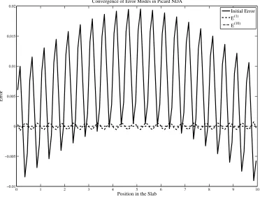
Figure 2.5 We see that both short- and long-wavelength error modes are damped quickly using Picard NDA. . . 39
Figure 3.1 x−y domain for 2D transport . . . 49
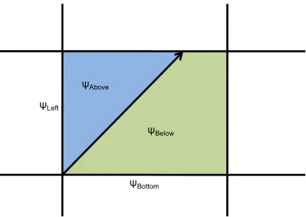
Figure 3.2 For µn > 0, ηn > 0, the cell-edge incoming angular fluxes denoted by red-circles are known since the boundary conditions are explicit. . . 51
Figure 3.3 For µn>0,ηn>0, the cell-edge fluxes denoted by red-circles are known since the boundary conditions are explicit. The cell-centered value, de-noted by the green diamond, can be computed using Equation 3.10. . . . 52
Figure 3.4 Given the cell-edge fluxes on the left and bottom boundaries along with the cell-averaged flux, we can compute the cell-edge fluxes, denoted by blue squares, on the top and right boundaries using Equations 3.8 and 3.9. 52 Figure 3.5 We proceed to the right across the first row computing the unknown cell-averaged and cell-edge fluxes. . . 53
Figure 3.6 Evaluating unknown fluxes in the second row of our grid. . . 53
Figure 3.7 Spatial domain with three explicit boundaries (single black line) and one reflective boundary (triple black line). . . 54
Figure 3.8 Particles encountering the reflective boundary with angle ˆΩ2 are reflected off in a new direction ˆΩ1. . . 55
Figure 3.9 Particles encountering the reflective boundary with angle ˆΩ2 are reflected off in a new direction ˆΩ1. . . 56
Figure 3.10 We must iterate on the incoming flux until we’ve reached an acceptable level of convergence when there is a pair of opposing reflective boundaries. 57 Figure 3.11 In this configuration the left and bottom boundaries are reflective and the remaining boundaries have explicit boundary conditions. . . 58
Figure 3.12 Configuration of cell for development of the step characteristics method. . 61
Figure 3.13 Source iteration damps high frequency error modes quickly, however low frequency errors persist. . . 69
Figure 3.14 NDA damps both high and low frequency error modes quickly. . . 70
Figure 4.1 Fissile region surrounded by two 5 m.f.p. reflectors. . . 86
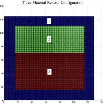
Figure 4.2 Three material reactor layout with regions labeled 1 - 3. . . 89
Figure 4.5 Plot of eigenvector corresponding to dominant eigenvalue for Zion reactor
problem. . . 94
Figure 4.6 LRA-BWR material layout with regions labeled 1 - 5. . . 95
Figure 4.7 Plot of eigenvector corresponding to dominant eigenvalue for LRA-BWR problem. . . 97
Figure 5.1 On the left we see the standard tally does not preserve balance, whereas on the right, the CED tally does an excellent job preserving balance using the same number of particles per simulation. . . 110
Figure 6.1 Comparing the scalar flux computed by a Monte Carlo transport sweep. . 116
Figure 6.2 Comparing the current computed by a Monte Carlo transport sweep. . . . 117
Figure 6.3 Comparing the consistency term computed by a Monte Carlo transport sweep. . . 118
Figure 6.4 Comparing the JFNK-NDA nonlinear residual in which a Monte Carlo transport sweep is used. . . 119
Figure 6.5 Noisy scalar flux before interpolation and after a least squares spline fit. . 120
Figure 6.6 Comparing the finite difference derivative of the scalar flux before and after LSS filtering. . . 121
Figure 6.7 Noisy scalar flux before interpolation and after a multi-spline filter appli-cation. . . 122
Figure 6.8 Comparing the finite difference derivative of the scalar flux before and after MS filtering. . . 123
Figure 6.9 Comparing the convergence of NDA(MC) using varying numbers of par-ticle per function evaluation. . . 124
Figure 6.10 Comparing the error in scalar fluxes computed using differing particle counts in NDA(MC) . . . 125
Figure 6.11 Comparing the residuals computed using AA-NDA(MC) . . . 126
Figure 6.12 Fluxes after 1, 2 and 3 runs of JFNK-NDA(MC) with increasing particle counts using standard tallies. . . 131
Figure 6.13 Nonlinear residuals after 1, 2 and 3 runs of JFNK-NDA(MC) with in-creasing particle counts using both Standard and CED Tallies. . . 132
Figure 6.14 KL= 5, η=.001,KR= 2 . . . 133
Figure 6.15 KL= 5, η=.001,KR= 1 . . . 133
Figure 6.16 KL= 10, η=.001, KR= 2 . . . 134
Figure 6.17 KL= 10, η=.001, KR= 1 . . . 134
Figure 6.18 KL= 5, η=.01,KR= 2 . . . 134
Figure 6.19 KL= 5, η=.01,KR= 1 . . . 134
Figure 6.20 KL= 10, η=.01,KR= 2 . . . 135
Figure 6.21 KL= 10, η=.01,KR= 1 . . . 135
Figure 6.22 KL= 5, η=.1,KR= 2 . . . 135
Figure 6.23 KL= 5, η=.1,KR= 1 . . . 135
Figure 6.24 KL= 10, η=.1,KR= 2 . . . 136
Figure 6.26 Both Standard and CED tallies achieve very efficient strong scaling across 40 nodes. 1011 particles per transport sweep were used. . . . 140
Figure 6.27 Material layout for 2-D Fixed-Source Problem. . . 145 Figure 6.28 Hybrid solution to the 2-D Fixed-Source Problem. . . 146 Figure 6.29 JFNK-NDA(MC) Convergence History for 2-D Fixed-Source Problem . . 147 Figure 6.30 The Shannon Entropy converges for the TMR problem. . . 149 Figure 6.31 The Shannon Entropy converges for the LRA-BWR problem. . . 150 Figure 6.32 The change in Shannon Entropy from iteration to iteration goes to zero
at the same rate as the error in the eigenvalue for the TMR problem. . . . 151 Figure 6.33 The change in Shannon Entropy from iteration to iteration goes to zero
at the same rate as the error in the eigenvalue for the LRA-BWR problem.152 Figure 6.34 On the left, we plot the group one and group two eigenvector, respectively.
On the right, we see the difference between the eigenvector computed using hybrid methods and deterministic methods. . . 153 Figure 6.35 We plot the four convergence metrics for the first simulation for the
LRA-BWR problem. . . 154 Figure 6.36 We plot the four convergence metrics for the second simulation for the
LRA-BWR problem. . . 154 Figure 6.37 On the left, we plot the group one and group two eigenvector, respectively.
On the right, we see the difference between the eigenvector computed using hybrid methods and deterministic methods. . . 155 Figure 6.38 We plot the four convergence metrics for the first simulation for the TMR
problem. . . 156 Figure 6.39 We plot the four convergence metrics for the second simulation for the
TMR problem. . . 156 Figure 6.40 We plot the nonlinear residual as a function of space for a 75×78 mesh. 159 Figure 6.41 We plot the nonlinear residual as a function of space for a 175×182 mesh.160 Figure 6.42 We plot the scaled one-norm of the nonlinear residual by iteration for a
series of three meshes. . . 161 Figure 6.43 On the left, we plot the group one and group two eigenvector, respectively.
On the right, we see the difference between the eigenvector computed using hybrid methods and deterministic methods. . . 162 Figure 6.44 We plot the four convergence metrics for the Zion reactor problem. . . 163 Figure 6.45 We plot the nonlinear residual as a function of space for a 136×136 mesh.164 Figure 6.46 We plot the nonlinear residual as a function of space for a 204×204 mesh.165 Figure C.1 Low-Order Solution Error Term Constants as a function of the scattering
ratio and domain length. . . 194 Figure C.2 Monte Carlo Error Term Constants as a function of the number of cells
and domain length. . . 196 Figure D.1 Convergence history of the eigenvalue using 40000 active cycles with 105
particles per cycle. . . 199 Figure D.2 Shannon Entropy history using 40000 active cycles with 105 particles per
Figure D.3 Change in Shannon Entropy from cycle to cycle using 40000 active cycles with 105 particles per cycle. . . 201
Figure D.4 Convergence history of the eigenvalue using 10000 active cycles with 106 particles per cycle. . . 202 Figure D.5 Shannon Entropy history using 10000 active cycles with 106 particles per
cycle. . . 203 Figure D.6 Change in Shannon Entropy from cycle to cycle using 5000 active cycles
with 106 particles per cycle. . . 204 Figure D.7 Convergence history of the eigenvalue using 1000 active cycles with 107
particles per cycle. . . 205 Figure D.8 Shannon Entropy history using 1000 active cycles with 107 particles per
cycle. . . 206 Figure D.9 Change in Shannon Entropy from cycle to cycle using 1000 active cycles
Chapter 1
Introduction
The goal of our work is to construct, or improve, methods for solving the neutron transport equation in the most efficient and precise manner possible. This equation governs the distri-bution of neutrons in space, angle and energy and its solution is essential for constructing and calibrating nuclear reactors, radiation shielding, medical imaging, and a wide range of other applications. Generally, we letψ(~r, E,Ω, t)ˆ dV dΩˆ dE dtdenote the total path length traversed by all particles within some differential volume dV about the position~r in R3, with energies
within dE about E, traveling in directionsdΩ about ˆˆ Ω during a time dt about t. In the most general case, the neutron transport equation is
1 v
∂ψ
∂t + ˆΩ· ∇ψ+ Σt(~r, E)ψ(~r, E,Ω, t)ˆ =
Z
4π dΩˆ0
Z ∞
0
dE0Σs(E0 →E,Ωˆ0 →Ω)ψ(~ˆ r, E0,Ωˆ0, t) + χ(~r, E, t)
4π
Z ∞
0
dE0 Z
4π
dΩˆ0 ν(~r, E0, t)Σf(~r, E0, t0)ψ(~r, E0,Ωˆ0, t) +s(~r, E,Ω, t),ˆ (1.1)
where~r = (x, y, z)T describes the position within the medium. ˆΩ describes the direction that particles are traveling. We represent integration over all directions in the following manner:
Z
4π
·dΩˆ ≡
Z 2π
0
Z π
0
· sin(θ)dθdω
The function sis a known source. We also must specify a boundary condition
For the time dependent form, we must also specify an initial condition:
ψ(~r, E,Ω,ˆ 0) =ψ0(~r, E,Ω).ˆ (1.3)
Before we continue, let’s discuss the derivation of the neutron transport equation [7].
1.1
Deriving the Transport Equation
Our goal in this study is to determine the distribution of neutrons in a system. Given some system configuration, we need to be able to accurately predict the balance of neutrons and this can be accomplished by solving the neutron transport equation. However, before we can use this equation, we must understand every piece of it. To aid in our understanding of the equation, we’ll go through a step by step derivation. We can describe the distribution of neutrons in space, angle, and energy by a functionn=n(~r, E,Ω, t).ˆ
The balance of neutrons in a reactor is governed by the material composition within the reactor as well as the way in which neutrons interact with matter, neutron sources and contri-butions from external boundaries. It should be clear that neutrons will interact differently with different materials based upon their physical structure. It will be beneficial in our study to begin this derivation by looking at several material properties that, in effect, help us describe the distribution of neutrons in a system.
1.1.1 Basic Definitions
When a neutron undergoes an interaction with matter, several things can happen. First, the neutron can scatter. By this we mean that the neutron hits a nucleus and bounces off with a new direction and energy. Secondly, a neutron can be absorbed by a nucleus. In some absorption reactions, the nucleus can undergo fission and produce more neutrons. For now, we’ll simply stick with these three options: scattering, absorption, and fission. We begin with a few definitions:
Definition 1. Σsis called the macroscopic scattering cross-section. Σsis equal to the probability
of undergoing a scattering reaction per unit path length traveled.
Definition 2. Σa is called the macroscopic absorption cross-section. Σa is equal to the
proba-bility of undergoing an absorption reaction per unit path length traveled.
Definition 3. Σf is called the macroscopic fission cross-section. Σf is equal to the probability
Definition 4. Σt is called the macroscopic total cross-section and is equal to Σs+ Σa. Σt can
be interpreted as the probability per unit path length traveled that a neutron will incur a reaction with a nucleus in the medium.
Let us discuss these three cross-sections in a bit more detail before moving on. First, it is important to note that Σs, Σa and Σt are all functions of energy, position, and time. In addition, Σs is a function of the incoming angle, as well as the post-interaction angle and energy. It makes sense that these quantities should differ for different materials that comprise the reactor. Furthermore, as the energy of a neutron changes, its speed changes and this will affect the probability of undergoing various types of reactions. Lastly, as time progresses, the material properties of the reactor will change. This is immediately clear when we consider the burn-up of fuel or heating of materials. For this reason, we usually represent Σt= Σt(~r, E, t) and follow a similar convention for Σsand Σa. The scattering cross-section has a more complicated representation and will be discussed in greater detail later.
In order to understand these cross-sections further, let us look at a simple example. Suppose Σs/Σa = 9. This tells us that on average, in an infinite medium a neutron will undergo 9 scattering interactions before it is absorbed. If Σs/Σa = 9, we can see that Σs/Σt =.9. This tells us that given an interaction, the probability that the neutron scatters is .9.
Let us further examine the quantity Σa. Σa refers to the probability of undergoing an absorption reaction per unit path length. Now, if we let v denote the speed of a particle, we can see that Σav is equal to the mean number of absorption reactions per second. If we have n neutrons percm3, Σavn is equal to the absorption reaction rate density, that is, the rate at which neutrons are being absorbed per cm3. Then, if V represents some volume in the reactor, V vΣanrepresents the loss rate in that volume due to absorption.
Let ν be equal to the average number of neutrons created per fission event. Then, the quantity V vΣfνn is equal to the fission production rate in V, or the rate at which neutrons are produced due to fission. This type of analysis will help us throughout our derivation of the neutron transport equation.
As previously mentioned, ˆΩ refers to the direction that a neutron travels. In general ˆΩ = ˆ
Ω(θ, ω) = [sin(θ) cos(ω),sin(θ) sin(ω),cos(θ)]T. We notice that ˆΩ is a unit vector in the direction of motion.
During a scattering reaction, it is common for both energy and direction to change. Gen-erally, we let E and ˆΩ represent the initial energy and direction, respectively, and E0 and ˆΩ0 denote the energy and direction after the collision. For this reason, Σs= Σs(E0 →E,Ωˆ0→Ω).ˆ However, we can break this scattering cross-section down into more understandable pieces.
change direction from ˆΩ0 to ˆΩ and change energy from E0 to E. Using our knowledge of probability, it is easy to see that
Z ∞
0
dE Z
4π
dΩPˆ (E0,Ωˆ0 →E,Ω) = 1.ˆ (1.4)
Now, we can see that Z ∞
0
dE Z
4π
dΩΣˆ s(E0 →E,Ωˆ →Ωˆ0) = Z ∞
0
dE Z
4π
dΩΣˆ s(E0)·P(E0,Ωˆ0 →E,Ω)ˆ = Σs(E0)
Z ∞
0
dE Z
4π
dΩP(Eˆ 0,Ωˆ0 →E,Ω)ˆ = Σs(E0)
1.1.2 Derivation
As was previously mentioned, n(~r,Ω, E, t) is the neutron density function, sometimes referredˆ to as the neutron distribution function. This function n is such that n(~r,Ω, E, t)ˆ d3r dΩˆ dE is equal to the expected number of particles in some volume d3r about~r, with energies indE
about E, traveling in directionsdΩ about ˆˆ Ω at time t.
In order to derive the transport equation, we need a balance relation describing the move-ment of neutrons in phase space. Let us define a volume in phase space, P. Our phase space consists of 3 variables (6 dimensions),~r, ˆΩ, andE. We will refer to the quantityd3r dΩˆ dEas the differential volume in phase space.
In its most basic form, the neutron balance equation can be given by: [change rate in P] = [neutrons enteringP]−[neutrons leaving P].
If we want to determine the number of neutrons in P, we can integrate n(~r,Ω, E, t) over theˆ spatial volume ∆V, range of directions ∆ ˆΩ and energy range ∆E. Let us define N(t) as the number of neutrons in P at timet.
N(t) = Z
∆V Z
∆E Z
∆ ˆΩ
n(~r,Ω, E, t)dˆ ΩdEdˆ 3r (1.5)
Now, we can represent the change rate in the phase volume P asdN/dt.
Methods in which neutrons can enter the phase volume P: 1. Neutrons can be supplied by an external source
3. Neutrons can scatter into the phase volume (inscattering)
4. Neutrons can leak into the phase volume (neutrons change location in space) Methods in which neutrons can leave the phase volume P:
1. Neutrons can scatter out of the phase volume (outscattering) 2. Neutrons can be absorbed in the phase volume
3. Neutrons can leak out of the phase volume (neutrons change location in space)
If we can describe the rate at which all of these gains and losses occur, we will have a balance relation describing the distribution of neutrons in phase space. We will derive some of these terms, while others will simply be given. For most terms, the derivations are quite similar. We’ll look at each term in the equation in terms of gains and losses.
Gains
1. External Source: This requires no formal derivation. This is simply a source term describing the rate at which neutrons enter the phase volume due to an specified external source. When solving the transport equation, this will be considered data like the mate-rial properties in the system. This source is described by:
Sext(~r,Ω, E, t) =ˆ
# of neutrons
cm3·M eV ·ster·sec (1.6)
whereM eV stands for mega-electron volts and ster stands for steradians, the SI unit of solid angle, the three-dimensional analog to radians which describe the span of an angle in the plane.
Now, the rate at which neutrons enter the phase box due to this external source is given by:
Z
∆V d3r
Z
∆E dE
Z δΩˆ
dΩˆ Sext(~r,Ω, E, t)ˆ (1.7) 2. Fission Source: Recall that Σf is equal to the number of interactions per unit path length of a neutron andv(E)Σf is equal to the interaction rate per neutron (herev=v(E) since the speed is exactly determined by the energy of a neutron as it is assumed to behave like a classical point particle) [21]. Now, the quantity
represents the fission rate in d3r about ~r caused by neutrons with energies within dE about E with directions dΩ about ˆˆ Ω at timet. Thus,
Z
∆V d3r
Z
∆E dE
Z δΩˆ
dΩˆ v(E)Σf(~r, E, t)n(~r,Ω, E, t)ˆ (1.9) describes the fission rate within the phase box. However, we are not just interested in the fission rate within the phase box, we are interested in the rate at which neutrons are produced due to fission within the phase box.
We can see that the number of neutrons produced due to fission events in d3r about ~r caused by neutrons with energies indE about E and with directionsdΩ about ˆˆ Ω at time tis given by
ν(~r, E, t)Σf(~r, E, t)v(E)n(~r,Ω, E, t)ˆ d3r dΩˆ dE (1.10) where, as a reminder to the reader, ν is the mean number of fission neutrons produced per fission event.
This is not enough to determine how many neutrons are entering the phase box, however. We must know more information about the neutrons being produced; we must know the direction they are traveling when they are produced as well as their energy. We can assume that the fission neutron directions are distributed isotropically. That is, there is no preference of direction for fission neutrons, or one could say that there is equal probability of having any initial direction when produced due to fission. However, fission neutrons may be born with a variety of energies, and this spectrum is described byχ(E). Therefore, χ(E)dE describes the fraction of fission neutrons born with energies in dE about E. Now, we’re able to described the rate at which neutrons enter the phase box due to fission. This quantity is given by:
Z
∆V d3r
Z
∆E dE
Z δΩˆ
dΩˆ χ(E) 4π Z ∞ 0 dE0 Z 4π
dΩˆ0 ν(~r, E0, t)Σf(~r, E0, t0)v(E0)n(~r,Ωˆ0, E0, t)
It is important to make the distinction in the above quantity,E0 describes the energy of the neutron causing the fission event, whileE describes the energy of the fission neutrons. 3. Inscattering: The term inscattering refers to neutrons which scatter into the phase volume. This essentially means that after undergoing a scattering reaction, the neutrons have angles in ∆ ˆΩ about ˆΩ and energies in ∆E about E. Given the previous derivations, this quantity is relatively easy to describe:
Z
∆V d3r
Z
∆E dE
Z
∆ ˆΩ
dΩˆ Z ∞
0
dE0 Z
4π
The term above describes the rate at which neutrons scatter into the phase box.
4. Leakage into the Phase Box: Leakage into and out of the phase box will be handled simultaneously in its own section.
Losses
1. Absorption: When neutrons undergo collisions, it is possible that the neutron is ab-sorbed. Recall that the quantity
Σa(~r, E, t)v(E)n(~r,Ω, E, t)ˆ
is the rate at which neutrons are absorbed per cm3. Therefore, the rate at which neutrons
are absorbed within the phase box is given by Z
∆V d3r
Z
∆E dE
Z
∆ ˆΩ
dΩ Σˆ a(~r, E, t)v(E)n(~r,Ω, E, t).ˆ
2. Outscattering: The termoutscattering refers to the loss of neutrons which begin inside the phase volume but leave the phase volume due to scattering. This quantity is far more simple than the inscattering term because we do not concern ourselves with the final direction and energy of the scattered neutrons. We only care about the rate at which neutrons scatter within the phase volume. While some neutrons may undergo a scatter and remain within the phase volume, this quantity is taken care of in the inscattering term.
We can describe the rate at which neutrons outscatter by Z
∆V d3r
Z
∆E dE
Z
∆ ˆΩ
dΩ Σˆ s(~r, E, t)v(E)n(~r,Ω, E, t).ˆ
Leakage
Instead of computing different quantities as far as gains and losses, we will instead derive one term that incorporates the net leakage of neutrons in our system.
Consider some arbitrary surface dS with unit normal vector e~n. We can describe the net rate at which neutrons cross the areadSaround~rhaving energies withindEaboutE, traveling in directions within dΩ about ˆˆ Ω at time tby
ˆ
Now, the rate at which neutrons leave the phase box is given by Z
S∆V
ds Z ∆E dE Z ∆ ˆΩ
dΩ ˆˆ Ω·e~n v(E)n(~r, E,Ω, t)ˆ
where S∆V denotes the surface of ∆V. If we apply the divergence theorem, we can get this quantity in more recognizable (and useful) terms:
Z
∆V d3r
Z
∆E dE
Z
∆ ˆΩ
dΩ ˆˆ Ω· ∇v(E)n(~r, E,Ω, t)ˆ
1.1.3 The Transport Equation
Now that we have all of our gains, losses and leakage terms, we can put it all together to form the neutron transport equation. We will write this as:
[rate of change] + [loss rate] = [gain rate]. (1.11) We have:
Z
∆V d3r
Z
∆E dE
Z
∆ ˆΩ
dΩˆ ∂n(~r, E,Ω, t)ˆ
∂t + ˆΩ· ∇v(E)n(~r, E, ˆ Ω, t)
+ Σs(~r, E, t)v(E)n(~r,Ω, E, t) + Σˆ a(~r, E, t)v(E)n(~r,Ω, E, t)ˆ =
Z
∆V d3r
Z
∆E dE
Z
∆ ˆΩ
dΩˆ Z ∞
0
dE0 Z
4π
dΩˆ0 Σs(~r, E0,Ωˆ0→E,Ω, t)v(E)n(~ˆ r,Ωˆ0, E0, t) +χ(E) 4π Z ∞ 0 dE0 Z 4π
dΩˆ0 ν(~r, E0, t)Σf(~r, E0, t0)v(E0)n(~r,Ωˆ0, E0, t)
+Sext(~r,Ω, E, t)ˆ Since ∆V, ∆E and ∆ ˆΩ are all arbitrary we can conclude that the two integrands are equivalent everywhere within our domain. Thus, we have
∂n(~r, E,Ω, t)ˆ
∂t + ˆΩ· ∇v(E)n(~r, E, ˆ Ω, t)
+ Σs(~r, E, t)v(E)n(~r,Ω, E, t) + Σˆ a(~r, E, t)v(E)n(~r,Ω, E, t)ˆ = Z ∞ 0 dE0 Z 4π
dΩˆ0 Σs(~r, E0,Ωˆ0 →E,Ω, t)v(E)n(~ˆ r,Ωˆ0, E0, t) +χ(E) 4π Z ∞ 0 dE0 Z 4π
dΩˆ0 ν(~r, E0, t)Σf(~r, E0, t0)v(E0)n(~r,Ωˆ0, E0, t)
Furthermore, we know that Σa+ Σs= Σt, we can simplify slightly ∂n(~r, E,Ω, t)ˆ
∂t + ˆΩ· ∇v(E)n(~r, E,Ω, t) + Σˆ t(~r, E, t)v(E)n(~r,Ω, E, t)ˆ =
Z ∞
0
dE0 Z
4π
dΩˆ0 Σs(~r, E0,Ωˆ0 →E,Ω, t)v(E)n(~ˆ r,Ωˆ0, E0, t) + χ(E)
4π Z ∞
0
dE0 Z
4π
dΩˆ0 ν(~r, E0, t)Σf(~r, E0, t0)v(E0)n(~r,Ωˆ0, E0, t) +Sext(~r,Ω, E, t)ˆ
Now, we see that most terms include the quantity v(E)n(~r, E,Ω, t). We generally simplifyˆ the transport equation by defining ψ(~r, E,Ω, t) =ˆ v(E)n(~r, E,Ω, t). ψˆ is referred to as the angular flux. Substituting this quantity into the transport equation yields the following integro-differential equation:
1 v(E)
∂ψ(~r, E,Ω, t)ˆ
∂t + ˆΩ· ∇ψ(~r, E,Ω, t) + Σˆ t(~r, E, t)ψ(~r, E,Ω, t)ˆ =
Z ∞
0
dE0 Z
4π
dΩˆ0 Σs(~r, E0,Ωˆ0 →E,Ω, t)ψ(~ˆ r, E0,Ωˆ0, t) +χ(~r, E, t)
4π
Z ∞
0
dE0 Z
4π
dΩˆ0 ν(~r, E0, t)Σf(~r, E0, t0)ψ(~r, E0,Ω, t) +ˆ Sext(~r,Ω, E, t)ˆ (1.12)
We will refer to Equation 1.12 as the three-dimensional, time-dependent, energy-dependent, angularly-dependent neutron transport equation, or the 3-D neutron transport equation for short.
1.1.4 Initial and Boundary Conditions
It is also important to develop boundary conditions for the neutron transport equation. We’ll focus primarily on three types of boundary conditions [21]:
1. Known surface source
2. Vacuum boundary conditions (no incoming neutrons) 3. Reflective boundary conditions
We’ll discuss each of these boundary conditions in the following sections. Known Incoming Surface Source
The first example of an explicit boundary condition comes from a known incoming surface source. In this case, we specify some distribution of neutrons for each~r on the boundary,
in which ˆn·Ωˆ <0 where ˆnis the outward directed normal to the surface at the point ~r. Vacuum boundary conditions are a second example of explicit boundary conditions and are special case of the known incoming surface source in which ˜ψ = 0. We will commonly use vacuum boundary conditions throughout our discussion for the remainder of this thesis.
Reflective Boundary Conditions
The only implicit boundary conditions which we will consider are reflective boundary conditions. In this case, the incoming flux from the boundary is set equal to the outgoing flux at the same location with the angle reflected [21]. Mathematically speaking, we write
ψ(~r,Ω, E, t) =ˆ ψ(~r,Ωˆ0, E, t), (1.14) in which~r is on the boundary, ˆn·Ωˆ <0 and
ˆ
n·Ω =ˆ −nˆ·Ωˆ0 and ( ˆΩ×Ωˆ0)·nˆ= 0. (1.15) Initial Condition
For the initial condition, we must simply describe the initial distribution of neutrons in phase space,
ψ(~r,Ω, E,ˆ 0) = ˜ψ(~r,Ω, Eˆ ). (1.16)
1.2
Discretizing the Transport Equation in Energy and Angle
In general, we cannot solve Equation 1.12 in its continuous form. For this reason, we must discretize the Equation 1.12 in time, energy, angle and space. For the majority of this thesis we will concern ourselves only with solving the time-independent problem, so let us drop the time dependence in Equation 1.12:
ˆ
Ω· ∇ψ(~r, E,Ω) + Σˆ t(~r, E)ψ(~r, E,Ω) =ˆ Z ∞
0
dE0 Z
4π
dΩˆ0 Σs(~r, E0,Ωˆ0 →E,Ω)ψ(~ˆ r, E0,Ωˆ0) +χ(E)
4π Z ∞
0
dE0 Z
4π
dΩˆ0 ν(~r, E0)Σf(~r, E0)ψ(~r, E0,Ω) +ˆ Sext(~r,Ω, E)ˆ (1.17)
1.2.1 Energy Discretization
and E0 is to be chosen sufficiently large such that the number of particles with energies higher
thanE0 may be disregarded.
We say that a neutron is in groupgif its energy lies in the interval [Eg, Eg−1]. Our goal with
the “multigroup” approximation is to determine the angular flux, ψ, in each of theG groups. We’ll define thegroup angular flux,ψg, by
ψg(~r,Ω) =ˆ
Z Eg−1
Eg
ψ(~r,Ω, E)ˆ dE≡
Z g
ψ(~r,Ω, E)ˆ dE. (1.18)
Furthermore, we wish to define the multi-group cross-sections in such a way that we preserve reaction (total, fission, scattering, absorption) rates in each group.
Now, the energy integrals in Equation 1.17 can be represented Z ∞
0
·dE0 = G X g0=1
Z g0
·dE0.
With this in mind, we’ll integrate Equation 1.17 over a single energy group, g, and we find ˆ
Ω· ∇
Z g
dE ψ(~r, E,Ω) +ˆ Z
g
dE Σt(~r, E)ψ(~r, E,Ω)ˆ
= G X g0=1
Z g dE Z g0 dE0 Z 4π
dΩˆ0 Σs(~r, E0,Ωˆ0→E,Ω)ψ(~ˆ r, E0,Ωˆ0)
+ Z g dE χ(E) 4π G X g0=1
Z g0
dE0 Z
4π
dΩˆ0 ν(~r, E0)Σf(~r, E0)ψ(~r, E0,Ω) +ˆ Z
g
dE Sext(~r,Ω, E)ˆ (1.19)
As in [21], let us suppose that the group angular fluxes are separable in energy. That is, ψ(~r,Ω, E) =ˆ f(E)ψg(~r,Ω),ˆ (1.20) for allE ∈[Eg, Eg−1]. We interpretf(E) as a normalized weighting function (a distribution of
the particles throughout the energy interval) such that Z
g
Now, we can substitute Equation 1.20 into Equation 1.19 and we obtain ˆ
Ω· ∇ψg(~r,Ω) +ˆ Z
g
dE Σt(~r, E)f(E)ψg(~r,Ω)ˆ
= Z
g
dE Sext(~r,Ω, E) +ˆ G X g0=1
Z g dE Z g0 dE0 Z 4π
dΩˆ0 Σs(~r, E0,Ωˆ0 →E,Ω)fˆ (E0)ψg(~r,Ωˆ0)
+ Z g dE χ(E) 4π G X g0=1
Z g0
dE0 Z
4π
dΩˆ0 ν(~r, E0)Σf(~r, E0)f(E0)ψg(~r,Ωˆ0) (1.21)
At this point, we’ll begin defining the new multi-group cross-sections by Σt,g(~r) =
Z g
f(E)Σt(~r, E) dE (1.22)
νgΣf,g(~r) = Z
g
f(E)ν(~r, E0)Σf(~r, E) dE (1.23) Σs,g0→g(~r,Ωˆ0·Ω)ˆ =
Z g
dE Z
g0
dE0f(E0)Σs(~r, E0→E,Ωˆ0·Ω),ˆ (1.24)
the multi-group fission spectrum by χg =
Z g
χ(E) dE (1.25)
and the group source term by
Sext,g(~r,Ω) =ˆ Z
g
Sext(~r,Ω, E)ˆ dE. (1.26)
Using Equations 1.22 - 1.26, we can simplify Equation 1.21 and obtain the multi-group transport equation
ˆ
Ω· ∇ψg(~r,Ω) + Σˆ t,gψg(~r,Ω) =ˆ Sext,g(~r,Ω) +ˆ G X g0=1
Z
4π
dΩˆ0 Σs,g0→g(~r,Ωˆ0 →Ω)ψˆ g0(~r,Ωˆ0)
+ χg 4π
G X g0=1
Z
4π
1.2.2 Angular Discretization
In multiple dimensions, we begin the angular discretization process by representing the angular flux in terms of spherical harmonics
ψg(~r,Ω) =ˆ
∞
X l=0
l X m=−l
Yl,m∗ ( ˆΩ)φml (~r) (1.28)
whereYl,m is given by [21]
Yl,m( ˆΩ) =
(2l+ 1)(l−m)! (l+m)! P
m
l (µ)eiωm (1.29)
in whichµis the cosine of the polar angle,θ, andωis the azimuthal angle from spherical coordi-nates. Spherical coordinates are the natural way to represent angles in three space dimensions. Here,Plm is the associated Legendre function defined by the formula
Plm(µ) = (−1)m(1−µ2)m/2 d m
dµmPl(µ) (1.30)
in which Pl0(µ) = Pl(µ), the lth Legendre polynomial. With this definition, we see that the spherical harmonics are orthogonal in the sense that
Z
dΩˆ Yl,m( ˆΩ)Yl∗0,m0( ˆΩ) = 4πδll0δmm0. (1.31)
Furthermore, the Legendre addition theorem [21] states
Pl(µ0) =Pl( ˆΩ·Ωˆ0) = l X m=−l
1 2l+ 1Y
∗
l,m( ˆΩ)Yl,m( ˆΩ0). (1.32)
Now, we may represent the group-to group scattering cross-section Σs,g0→g(~r,Ωˆ0·Ω) in termsˆ
of Legendre polynomials
Σs,g0→g(~r, µ0) = ∞
X l=0
Σs,l,g0→g(~r)Pl(µ0), (1.33)
Finally, we may represent the scattering term in Equation 1.27 by G
X g0=1
Z g dE Z g0 dE0 Z 4π
dΩˆ0 Σs(~r, E0,Ωˆ0 →E,Ω)fˆ (E0)ψg(~r,Ωˆ0)
= ∞ X l=0 l X m=−l
Yl,m∗ ( ˆΩ) G X g0=1
Σs,l,g0→gφg 0
l,m(~r) (1.34)
whereφgl,m0 is given by
φgl,m= Z
4π
dΩˆ Yl,m( ˆΩ)ψg(~r,Ω).ˆ (1.35)
We’ll use this new representation of the scattering term for Equation 1.27 before discretizing in angle:
ˆ
Ω· ∇ψg(~r,Ω) + Σˆ t,gψg(~r,Ω) =ˆ Sext,g(~r,Ω) +ˆ
∞
X l=0
l X m=−l
Yl,m∗ ( ˆΩ) G X g0=1
Σs,l,g0→gφg 0
l,m(~r)
+χg(~r) 4π
G X g0=1
Z
4π
dΩˆ0 νgΣf,g0(~r)ψg0(~r,Ω).ˆ (1.36)
At this point, we are ready to begin the angular discretization of the transport equation given by Equation 1.36. We will use the discrete ordinates (Sn) method for discretizing in angle. Using this method, we consider the transport equation evaluated only at a finite set of angles ˆΩn = (µn, ηn, ξn)1 such thatµ2n+η2n+ξn2 = 1. We wish to handle reflective boundary conditions with ease so we demand that if ˆΩn = (µn, ηn, ξn) is in our quadrature set, so is
ˆ
Ωn0 = (±µn,±ηn,±ξn)
Furthermore, we would like to retain solution invariance under 90◦ rotations for problems with this type of rotational symmetry. Therefore, if the angle ˆΩ = (a, b, c) is in our angular quadrature set, so must be (a, c, b), (b, a, c), (b, c, a), (c, a, b) and (c, b, a). With this plane- and rotational symmetry in mind, we can choose a set ofN angles in the first octant and use these symmetry rules to produce the angles in the other octants.
Once our quadrature set has been chosen, we can represent the transport equation along
1In this definition,µ
nis not the polar angle used to define the spherical harmonics. This notation has been used to remain consistent with the popular text [21]. Relating this notation, we have µn =
p
1−µ2cos(ω),
ηn= p
1−µ2sin(ω), andξ
these 8N (or in 2-D, 4N) discrete angles. This yields a system of equations,
ˆ
Ωn· ∇ψg,n(~r) + Σt,gψg,n(~r) =Sext,g,n(~r) +
∞
X l=0
l X m=−l
Yl,m∗ ( ˆΩn) G X g0=1
Σs,l,g0→gφg 0
l,m(~r)
+ χg 4π
G X g0=1
8N X
i=1
dΩˆ0 νgΣf,g(~r)ψg,n(~r)wn. (1.37)
where
ψg,n(~r) =ψg(~r,Ωˆn) (1.38) and thewn’s are the associated quadrature weights.
Now, Equation 1.37 is ready for spatial discretization. This will be handled in Chapters 2 and 3 for one- and two-dimensional Cartesian geometries, respectively. In the case of isotropic scattering, Equation 1.37 simplifies dramatically:
ˆ
Ωn· ∇ψg,n(~r) + Σt,gψg,n(~r) = Sext,g,n(~r) +
1 4π
G X g0=1
Σs,g0→gφg0(~r) +χg(~r)
4π G X g0=1
νg0Σf,g0(~r)φg0(~r). (1.39)
We callφ(~r) thescalar flux. The scalar flux is the zeroth angular moment of the angular flux, given by
φ(~r) = Z
4π
dΩˆ ψ(~r,Ω).ˆ (1.40)
Furthermore, suppose that ψ depends spatially only on a single variable, z. In this case, the transport equation simplifies to the one-dimensional case
µ ∂
∂zψg(z, µ) + Σt,gψg(z, µ) =Sext,g(z, µ) + 1 2
G X g0=1
Σs,g0→gφg0(z) +χg
2 G X g0=1
νg0Σf,g0φg0(z).(1.41)
We’ll refer to Equation 1.41 as the one-dimensional neutron transport equation with isotropic scattering.
1.3
The
k
-eigenvalue Problem
When analyzing a nuclear reactor it is vital to determine the criticality which we quantify using the multiplication factor, kef f, of the reactor [23, 17, 21]. If kef f > 0, the reactor is supercritical, meaning that neutrons are being produced faster than they are being destroyed. If kef f = 1, the reactor is critical and the number of neutrons in each generation remains constant. If kef f <0, the reactor is subcritical.
We can compute kef f by determining the largest value of k which satisfies the following problem for some non-zero angular flux:
ˆ
Ω· ∇ψ(~r, E,Ω) + Σˆ t(~r, E)ψ(~r, E,Ω)ˆ =
Z ∞
0
dE0 Z
4π
dΩˆ0 Σs(~r, E0,Ωˆ0 →E,Ω)ψ(~ˆ r, E0,Ωˆ0) + χ(~r, E)
4πk Z ∞
0
dE0 Z
4π
dΩˆ0 ν(~r, E0)Σf(~r, E0)ψ(~r, E0,Ω).ˆ (1.42)
1.4
Organization of this Thesis
In Chapter 2, we explore methods for solving the 1-D steady-state neutron transport equation. We begin the chapter by deriving the integral transport equation before discussing the spatial discretization of the transport equation. From here, we introduce source iteration, the most simple method for solving the steady-state neutron transport equation. At this point, we’ll begin discussing methods for accelerating the solution to the transport equation.
In Chapter 3, we repeat our work from Chapter 2 in 2-D. The majority of this chapter deals with the two-dimensional spatial and angular discretizations and the method for executing a 2-D transport sweep.
In Chapter 4, we consider various methods for computing the dominant eigenvalue, kef f, as in Equation 1.42. Much like Chapter 2, we begin by discussing the most simple method for computing kef f known as power iteration. Then, we’ll look at several methods for accelerating the convergence of the eigenvalue.
In Chapter 5, we look at stochastic methods for solving the neutron transport equation. We begin with motivating the choice to incorporate Monte Carlo simulations in the solution of the transport equation. We first look at solving a 1-D steady-state transport problem using Monte Carlo methods. Next, we look at representing a transport sweep using a Monte Carlo simulation.
Chapter 2
Deterministic Solutions to the 1-D,
Mono-energetic Transport Equation
in Slab Geometry
In this chapter we will consider several methods for solving the one-dimensional, fixed-source neutron transport equation in slab geometry. We will begin by deriving the integral equation for 1D neutron transport. From here, we will begin the discussion of solution methods with source iteration, as it is the simplest solution method and an understanding of source iteration is prerequisite for all other methods. Once source iteration has been implemented and we are comfortable with the idea of a transport sweep, we will begin developing more advanced methods. We’ll attempt to accelerate convergence using both known mathematical acceleration techniques alongside physics-based accelerators. All of the accelerators use transport sweeps at the heart of the algorithm.
2.1
Problem Definition
In this chapter we will focus our attention to solving the mono-energetic 1-D neutron transport equation in slab geometry with isotropic scattering:
µ∂ψ
∂x(x, µ) + Σtψ(x, µ) = 1
2[Σsφ(x) +Q(x)] (2.1)
forx ∈(0, τ) where ψ(x, µ) is the angular flux at the point x traveling in the directionµ. We have the following boundary conditions:
These boundary conditions essentially describe the number of particles entering from the left end of the slab and the number of particles entering from the right side of the slab.
The direction cosine µis given by µ=cos(θ). The relationship between µand θ can seen in Figure 2.1.
Figure 2.1: Slab of width τ
Our goal is to solve this problem in an iterative manner to a high degree of accuracy with as little computational effort as possible.
2.2
Source Iteration
In order to solve Equation 2.1 we propose an iterative scheme: 1. Begin with an initial guessφ0(x).
2. Givenφ0(x), solve Equation 2.1 forψ1(x, µ).
3. Letφ1(x) =
R1
−1ψ1(x, µ)dµ.
4. Continuing this iteration until successive functionsφare sufficiently “close” yields a solu-tion. That is, givenφn(x), computeψn+1(x). Then computeφn+1(x) =
R1
2.2.1 Deriving the Integral Transport Equation
Before describing the source iteration algorithm in greater detail, let us motivate this action by deriving the integral transport equation in one-dimension. We’ll perform an analysis along the same lines as found in [16]. For simplicity, let us assume that both the total and scattering cross-sections are constant.
We begin by manipulating the transport equation using a linear change of variables. Letting z= Σtx, we have
µΣt
∂ψ(z, µ)
∂z + Σtψ(z, µ) = 1
2[Σsφ(z) +Q(z)].
Now, dividing both sides by the total cross section, Σt, and letting c = Σs/Σt and S(x) = Q(x)/Σt, we find
µ∂ψ
∂z +ψ(z, µ) = 1
2[cφ(z) +S(z)] (2.3)
Here, sincex∈[0, τ], we must have z∈[0, X] whereX=τ /Σt.
Now, returning back to x as our spatial variable, for positive µwe compute: µ∂ψ
∂x +ψ(x, µ) = 1
2[cφ(x) +S(x)] exµ
µ∂ψ
∂x +ψ(x, µ)
= exµ1
2[cφ(x) +S(x)] µ ∂
∂x h
exµψ(x, µ)
i
= 1 2e
x
µ[cφ(x) +S(x)]
∂ ∂x
h
exµψ(x, µ)
i
= 1
2µe
x
µ[cφ(x) +S(x)]
Z y
0
∂ ∂x
h
eµxψ(x, µ)
i dx = Z y 0 1 2µe x
µ[cφ(x) +S(x)]dx
eµyψ(y, µ)−ψ(0, µ) =
Z y
0
1 2µe
x
µ[cφ(x) +S(x)]dx
ψ(y, µ) = e−
y µ Z y 0 1 2µe x
µ[cφ(x) +S(x)]dx+e− y µF
0(µ)
ψ(y, µ) = Z y
0
1 2µe
(x−y)
µ [cφ(x) +S(x)]dx+e− y
µF
0(µ)
ψ(y, µ) = Z y
0
1 2µe
−|x−y|
|µ| [cφ(x) +S(x)]dx+e−
y
|µ|F
For negative µ, we integrate backwards and obtain a similar expression:
ψ(y, µ) = −
Z X y
1 2µe
(x−y)
µ [cφ(x) +S(x)]dx+e
(X−y)
µ F
X(µ) ψ(y, µ) =
Z X y
1 2|µ|e
−|x−y|
|µ| [cφ(x) +S(x)]dx+e −|X−y|
|µ| F
X(µ)
Now, we can transform these two equations for ψ into a single relation for φ by noticing that
φ(x) = Z 1
−1
ψ(x, µ)dµ
= Z 1
0
ψ(x, µ) dµ+ Z 0
−1
ψ(x, µ) dµ. (2.4)
Applying Equation 2.4, we have
φ(y) = Z 1 0 Z y 0 1 2µe
−|x−y|
|µ| [cφ(x) +S(x)]dxdµ+
Z 1
0
e−
y
|µ|F
0(µ)dµ + Z 0 −1 Z X y 1 2|µ|e
−|x−y|
|µ| [cφ(x) +S(x)]dxdµ+
Z 0
−1
e
−|X−y|
|µ| F
X(µ)dµ. We can split both the first and third terms in the above expression into two integrals:
φ(y) = Z 1 0 Z y 0 1 2µe
−|x−y|
|µ| cφ(x)dxdµ+
Z 1 0 Z y 0 1 2µe
−|x−y|
|µ| S(x)dxdµ
+ Z 1
0
e−
y
|µ|F
0(µ)dµ+
Z 0
−1
Z X y
1 2|µ|e
−|x−y|
|µ| cφ(x)dxdµ
+ Z 0 −1 Z X y 1 2|µ|e
−|x−y|
|µ| S(x)dxdµ+
Z 0
−1
e
−|X−y|
|µ| F
X(µ)dµ.
Now, we can combine the integrals containing the scalar flux and source by switching the order of integration:
φ(y) = Z X 0 Z 1 0 1 2ηe
−|x−y|
η cφ(x)dηdx+
Z X 0 Z 1 0 1 2ηe
−|x−y|
η S(x)dηdx
+ Z 1
0
e−
|y| |µ|F
0(µ)dµ+
Z 0
−1
e
−|X−y|
|µ| F
X(µ)dµ.
Finally, we rearrange terms and are left with following integral equation:
φ(y)−
Z X
0
where
k(x, y) = c
2E(|x−y|) E(|x−y|) =
Z 1
0
1 ηe
−|x−y|
η dη
g(y) = Z X
0
1
2E(|x−y|)S(x) dx+ Z 1
0
e−
y ηF
0(η)dη+
Z 1
0
e
−|X−y|
η F
X(−η)dη. At this point, it is easy to see that solving the transport equation is equivalent to solving the following integral equation:
φ+K(φ) = g where
K(φ(x)) = Z X
0
k(x, y)φ(x) dx.
Now, we realize source iteration by
φ(n+1) = K(φ(n)) +g.
It is important to show that source iteration converges when the domain is finite andc <1. We state this as a theorem as the result provides a backbone for the remainder of this thesis. Theorem 1. Source iteration will converge whenever either X <∞ or c <1. [6]
Proof. We wish to show that kKk<1 for some choice of operator norm. Then, by Theorem 4 (Appendix A), the iteration will converge.
We will proceed by using the 1-norm, given by
kuk=kuk1≡
Z X
0
|u(x)|dx.
Now, we will prove Theorem 1 by showing that
We have,
Z X
0
|K(φ)(y)|dy = Z X 0 Z X 0 k(x, y)φ(x)dx dy ≤ Z X 0 Z X 0
|k(x, y)||φ(x)|dx dy
= Z X
0
Z X
0
|k(x, y)||φ(x)|dy dx
= Z X
0
|φ(x)|
Z X
0
|k(x, y)|dy dx = c 2 Z X 0
|φ(x)|
Z X
0
|E1(|x−y|)|dy
dx = c 2 Z X 0
|φ(x)|
Z X
0
E1(|x−y|)|dy
dx (2.5) ≤ c 2 Z X 0
|φ(x)|
Z ∞
−∞
E1(|x−y|)dy
dx (2.6) = c 2 Z X 0
|φ(x)|
Z ∞
−∞
E1(|z|)dz
dx = c 2 Z X 0
|φ(x)|dx Z ∞
−∞
E1(|z|)dz
= c 2kφk
Z ∞
−∞
E1(|z|)dz. (2.7)
Furthermore, we can see that Z ∞
−∞
E1(|z|)dz = 2
Z ∞
0
E1(y)dy
= 2 Z ∞ 0 Z 1 0 1 ηe
−y/ηdηdy
= 2 Z 1 0 1 η Z ∞ 0
e−y/ηdy dη = 2 Z 1 0 1 η ·η dη = 2
Z 1 0
1 dη
Combining the results from Equations 2.7 and 2.8, we have
kKφk ≤ c
2kφk · Z ∞
−∞
E1(|z|)dz
= c 2kφk ·2 = ckφk
Now, if c < 1, we have kKk < 1 and the iteration converges. Furthermore, if φ(x) is non-zero everywhere, we see that the inequality between Equations 2.5 and 2.6 should be a strict inequality when X <∞. Therefore, whenX <∞, we have kKk<1 even if c= 1.
2.2.2 Discretizing the Transport Equation
In order to solve the transport equation with source iteration, we need a method for computing φ(n+1) given φ(n). To do this, we must discretize the transport equation and iterate on the
discrete solution. Before introducing the discretized equations, let us familiarize ourselves with the domain. Consider Figure 2.2:
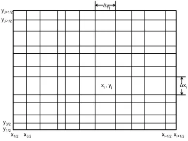
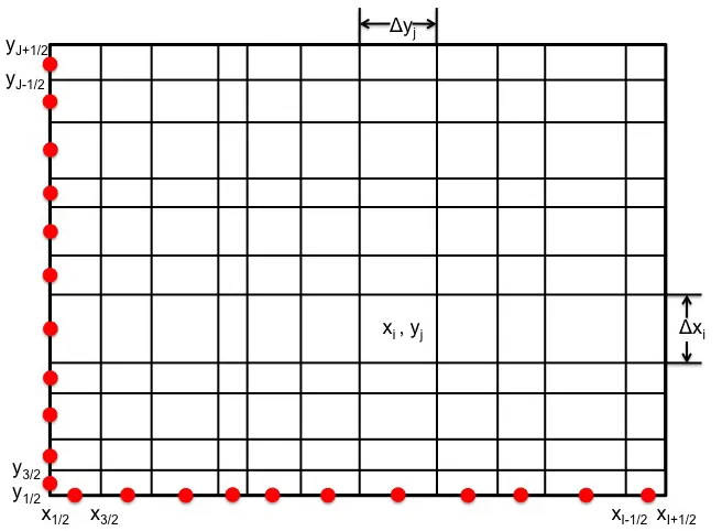
Figure 2.2: Cell faces take on half-integer indices and cell-centers take on integer indices.
In 1-D, we may choose to compute fluxes at either cell faces or cell centers. For the remainder of this chapter, let us choose to compute cell-face values of the angular flux. We’ll compute the angular flux at all grid-points with half-integer values (ψi+1
2 =ψ(xi+ 1
2)). Furthermore, we
will compute the scalar flux at cell centers (φi=φ(xi)). In this case, φi represents the average scalar flux over theith cell.
This choice of stencil leads to the following diamond difference discretization [2]:
µk ψk
i+12 −ψ
k i−1
2
∆xi
+ Σt ψk
i+12 +ψ
k i−1
2
2 = Σsφi+qi (2.9)
φi = X
k wk
ψi−1 2 +ψi+
1 2
2
!
whereψki+1 2
=ψ(xi+1
2, µk) and ∆xi=xi+ 1 2
−xi−1
2. Theµk’s are chosen to be Gauss nodes and
thewk’s as their corresponding weights.
For positive µk, we can solve Equation 2.9 forψki+1 2
:
ψki+1 2
=
µk ∆xi −
Σt 2
ψik−1
2
+ Σsφi+qi µk
∆xi + Σt
2
(2.11)
Now, given an explicit boundary condition on the left boundary (x = 0), we can march across the domain. Similarly, for negative µk we can solve Equation 2.9 for ψik−1
2
. This allows us to propagate information across the domain beginning from the right boundary (x = X). This idea is referred to as a “transport sweep” and can be visualized in Figure 2.3:
Figure 2.3: For µ > 0, information propogates across the medium originating from the left boundary. Forµ <0, information from the right boundary is propogated across the medium.
2.2.3 Analyzing Source Iteration
Source iteration converges whenever the width of the slab is finite and/or the ratio Σs/Σt<1, however we are not guaranteed that source iteration will converge in a timely manner. When Σs/Σt ≈ 1 and the mean-free-path (1/Σt) of a neutron is far shorter than the width of the slab, convergence may take hundreds or thousands of iterations to converge [2]. Since each iteration is on the order of n·kwork, this can be quite expensive, and recall, this is for a 1-D calculation. Each iteration will become more expensive as we reach higher dimensions, add in multiple energy groups and assume anisotropic scattering.
The following theorem helps us to quantify how poorly source iteration may perform in certain problem regimes.
Theorem 2. Suppose Equation 2.1 for x∈[−∞,∞] has a solution ψ∗(x, µ). Define an error function,e(k)(x, µ) =ψ∗(x, µ)−ψ(k)(x, µ) where the ψ(k) are the sequence of iterates produced by source iteration. Then we have
e
(k)(x, µ)
≤B·c
k (2.12)
where B is a constant determined by the initial error and c= Σs/Σt is the scattering ratio.
Proof. We’ll prove this theorem using the method described in [2]. Consider the exact transport equation (Equation 2.13) and the source iteration scheme (Equation 2.14) for an infinite medium (x∈[−∞,∞]),
µ∂ψ
∗
∂x (x, µ) + Σtψ
∗(x, µ) = 1
2
Σs Z 1
−1
ψ∗(x, µ0)dµ0+Q(x)
(2.13)
µ∂ψ
(k+1)
∂x (x, µ) + Σtψ
(k+1)(x, µ) = 1
2
Σs Z 1
−1
ψ(k)(x, µ0)dµ0+Q(x)
. (2.14)
Subtracting Equation 2.14 from 2.13 yields the following equation for the error
µ∂e
(k+1)
∂x (x, µ) + Σte
(k+1)(x, µ) = 1
2
Σs Z 1
−1
e(k)(x, µ0)dµ0
. (2.15)
Equation 2.15 relates the current error to the previous error, and iteratively, the current error to the initial error.
Now, consider expanding the kth error, e(k), as a Fourier integral, e(k)(x, µ) =
Z ∞
−∞
Substituting Equation 2.16 into Equation 2.15, we have Z ∞
−∞
Σt(iλµ+ 1)A(k+1)(λ, µ)− Σs
2 Z 1
−1
A(k)(λ, µ0)dµ0
eiΣtλxdλ= 0. (2.17)
Therefore, we must have
A(k+1)(λ, µ) = c 2
1 1 +iλµ
Z 1
−1
A(k)(λ, µ0)dµ0 (2.18)
forλ∈Rand forµ∈[−1,1]. We assume thatc <1 so that Theorem 1 guarantees convergence.
Integrating Equation 2.18 over all µyields Z 1
−1
A(k+1)(λ, µ0)dµ0=ω(λ) Z 1
−1
A(k)(λ, µ0)dµ0 (2.19)
in which
ω(λ) ≡ c
2 Z 1
−1
1
1 +iλµdµ (2.20)
= c Z 1
0
1
1 +λ2µ2dµ (2.21)
= c λtan
−1λ. (2.22)
Then, for allk≥0, Equation 2.19 implies Z 1
−1
A(k)(λ, µ0)dµ0 =ω(λ)k Z 1
−1
A(0)(λ, µ0)dµ0 (2.23)
Applying Equation 2.18 to the left-hand side of Equation 2.23 yields
A(k+1)(λ, µ) = c 2
ωk 1 +iλµ
Z 1
−1
A(0)(λ, µ0)dµ0
(2.24)
Now, we have an explicit formula for the error based on the initial error for all k ≥0, as given by
e(k+1)(x, µ) = Z ∞
−∞
c 2
ωk 1 +iλµ
Z 1
−1
A(0)(λ, µ0)dµ0
We can bound the (k+ 1)st error as follows,
e
(k+1)(x, µ) ≤
c 2
Z ∞
−∞
|ω(λ)|k
Z 1 −1
A(0)(λ, µ0)dµ0 dλ = c 2 Z ∞ −∞ Z 1 −1
A(0)(λ, µ0)dµ0 dλ
σSIk
= B·σSIk , (2.26)
whereB is a constant based on the Fourier expansion coefficient of the initial error and spectral radius of the source iterations scheme is given by
σSI = max λ∈R
ω(λ) = max λ∈R
c λtan
−1λ=ω(0) =c. (2.27)
Clearly, asc→1 and in the case of an infinite medium, the iteration may become arbitrarily slow. When c =.99, it will take over 200 iterations to decrease the error by a single order of magnitude. When c = .999, over 2000 iterations will be required to decrease the error by an order of magnitude. This helps motivate us to put forth effort in developing efficient and robust accelerators to solve the neutron transport equation.
Before moving on, we can perform further analysis of the source iteration scheme that will aid us in building these accelerators. As in [2], let us assume that the initial error consists of a single Fourier mode,
e(0)(x, µ) =a(µ)e−Σtλx. (2.28)
Then, for all iterates k ≥0, the error is comprised of this single Fourier mode and the above derivation demonstrates
e(k+1)(x, µ) = ωk(λ)
c 2
1 1 +iλµ
Z 1
−1
a(µ0)dµ0
eiΣtλx. (2.29)
Source iteration will converge slowest for modes in which λ is nearly 0. In other words, the slowest converging components of the solution have weak spatial dependence, or are the long-wavelength components of the solution [2].
this solution,
φ(0)=φ∗(x) +.01 sinπx τ
+.01 sin
40πx τ
.
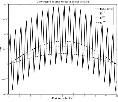
Figure 2.5 shows the initial error along with the error after 25, 50, and 100 iterations.
0 1 2 3 4 5 6 7 8 9 10
−0.01 −0.005 0 0.005 0.01 0.015 0.02
Position in the Slab
Error
Convergence of Error Modes in Source Iteration
Initial Error
E(25)
E(50)
E(100)
Figure 2.4: We see that the long wavelength error mode converges at a much slower rate than the short wavelength error mode.
of the solution, as standard source iterations will quickly resolve the high-frequency modes, while simultaneously ensuring that high-frequency errors are not amplified.
2.3
Using Krylov Methods to Solve the Transport Equation
In general, source iteration is not a feasible method for solving the neutron transport equation. Even for relatively simple problems, one energy group and 1-D, these problems can require thousands of iterations in order to converge to the desired tolerance. For this reason, we need to employ more advanced methods to cut down on the amount of work required to obtain a solution. In the nuclear engineering community, algorithms which attempt to cut down the number of transport sweeps required to converge are often referred to as “accelerators.”
In order to utilize Krylov methods to solve this problem, we need to represent this problem as a linear system of equations. Early in this chapter we showed that we could represent source iteration using operator notation as:
φ(n+1) = K(φ(n)) +g (2.30) whereK is a linear operator.
Equation 2.30 has converged ifφ(n)=φ(n+1). Instead of using source (or Picard) iteration to solve this problem, we should be able to increase the rate of convergence by using Krylov meth-ods. In this case, we’ll describe the problem slightly differently, writing the integral equation as:
φ(x)− K(φ)(x) = g(x) (2.31)
(I− K)φ(x) = g(x) (2.32)
whereI is the identity function.
Once we discretize, this becomes a linear system of equations
A~φ=~g. (2.33)
whereA comes from the discretization of I− K.
2.3.1 GMRES
One of the most common Krylov methods is GMRES, which stands for Generalized Minimum RESidual. When solving A~x=~b, GMRES minimizes||~b−A~x||2 over the spacex0+Kk, where Kk denotes thekth Krylov subspace [15]. This is defined as
Kk= span(r0, Ar0, ...Ak−1r0) (2.34)
GMRES is guaranteed (in the absence of roundoff error) to converge in nor less iterations when the dimension of the problem is n (i.e. x is a vector of length n). We prove this fact in Appendix A.
For well-conditioned problems (problems where K(A) = ||A|| · ||A−1|| ≈ small), GMRES can converge quite quickly. The convergence behavior is determined by the spectrum of A, or the set of eigenvalues of A. It can be shown ([1]) that GMRES performs best when these eigenvalues are grouped in a few tight clusters.
The other selling point for GMRES is that we do not actually need to form the matrix A. Instead, we only need a matrix-vector-product (hereafter referred to as a “matvec”), that is, a routine that can compute the action of A on a vector. For the neutron transport problem, creating the actual matrix could require far too much work to be a reasonable solution, so we can take advantage of this property of GMRES. A more detailed discussion of GMRES can be found in Appendix A.
2.3.2 Building the Matrix-Vector-Product
For the neutron transport problem, our matvec is straightforward to build. Our matvec, M, must represent the action of (I− K) on a vector. The matrix, M, is simply the discrete version of the operator (I− K).
If we recall our discussion of source iteration, we have a mapping that takes φl toφl+1. We can represent this asG(φl) =φl+1. We’ve found our solution whenG(φ) =φ. Furthermore, in the previous section, we found thatφ=Kφ+b. Combining these two facts, we can see that
G(φ) =Kφ+b. (2.35)
Therefore, the action of A on a vector can be represented asKφ=G(φ)−b. If we need to computeb, we can see thatb=G(~0).
Now, our matvec, M, can be explicitly defined: