Further Development of the Application of Adaptive Model Refinement to Nuclear Reactor Core Simulation

(1)

ABSTRACT

ALDRIDGE, BETH ELLEN. Further Development of the Application of Adaptive Model Refinement to Nuclear Reactor Core Simulation. (Under the direction of Paul Turinsky.)

Designing the core of a nuclear power reactor is an intricate process, as there are many requirements that must be met. In order to ensure that the reactor can be operated safely, it is important to be able to predict the behavior of the core. Computational simulations of reactor behavior are based on mathematical models that can meet nearly any desired level of fidelity, though higher fidelity usually comes with a higher computational cost. There are many techniques available for optimizing the fidelity to cost ratio. This work explores and further develops the Adaptive Model Refinement (AMoR) technique introduced in the Master’s thesis of Sterling Satterfield [1]. The AMoR technique is designed to integrate two or more different fidelity simulation models to create a hybrid model which can provide high accuracy solutions faster. This proof of concept for applying AMoR to nuclear reactor neutron simulation employs as low-fidelity a point reactor kinetics solver (PKE-Solver) and as high-fidelity, the few-group diffusion code NESTLE [2]. The low-fidelity model uses an adaption of the Quasi-Static method [3] to convert the PKE-solver results into a 3-dimensional flux and delayed neutron precursor solution. The adaptation is based on the concept of the flux being separable into amplitude and shape functions. The low-fidelity solution is compared to the high fidelity solution via assorted error metrics.

(2)

(3)

Further Development of the Application of Adaptive Model Refinement to Nuclear Reactor Core Simulation

by

Beth Ellen Aldridge

A thesis submitted to the Graduate Faculty of North Carolina State University

in partial fulfillment of the requirements for the Degree of

Master of Science

Nuclear Engineering

Raleigh, North Carolina 2015

APPROVED BY:

_______________________________ _______________________________

Dmitriy Anistratov Robert White

_______________________________ Paul Turinsky

(4)

ii

BIOGRAPHY

(5)

iii

LIST OF FIGURES

Figure 1: Required runs in NESTLE and PKE-solver to produce a full high-fidelity vs.

low-fidelity comparison in the original and current AMoR setups. ...13

Figure 2: Original low-fidelity AMoR setup. ...14

Figure 3: AMoR input to GPT responses...21

Figure 4: Maximum flux error for 25 steady-state projection operator sets. ...24

Figure 5: Hot-spot flux error for 25 steady-state projection operator sets. ...25

Figure 6: Maximum flux error for 0.002 second rapid-insertion projection operator sets. ...25

Figure 7: Hot-spot flux error for 0.002 second rapid-insertion projection operator sets. ...26

Figure 8: Maximum precursor error for 25 steady-state projection operator sets. ...27

Figure 9: RMS precursor error for 25 steady-state projection operator sets. ...27

Figure 10: Maximum precursor error for 0.002 second rapid-insertion projection operator sets. ...28

Figure 11: RMS precursor error for 0.002 second rapid-insertion projection operator sets. ...28

Figure 12: Maximum precursor error for rapid-insertion projection operators hybrid method. ...30

Figure 13: RMS precursor error for rapid-insertion projection operators hybrid method. ...30

Figure 14: RMS flux error for 0.002 second rapid-insertion projection operators hybrid method, with one switch halfway through the 2 second transient. ...31

Figure 15: RMS flux error for rapid-insertion projection operators with suppressed DNPs and projected precursors method, with one switch halfway through the 2 second transient. ...32

Figure 16: Neutron flux vs. Rod Height at a non-rodded location. ...33

Figure 17: Neutron flux vs. Rod Height, zoomed in, at a non-rodded location. ...34

Figure 18: Current AMoR setup ...36

Figure 19: 2 second rod withdrawal transient average neutron density. ...38

Figure 20: 2 second rod withdrawal transient maximum flux error. ...38

Figure 21: 2 second rod withdrawal transient RMS flux error. ...39

Figure 22: 2 second rod withdrawal transient maximum precursor error. ...39

Figure 23: 2 second rod withdrawal transient RMS precursor error. ...40

Figure 24: 2 second rod insertion, RMS flux-shape error extended ...41

Figure 25: 2 second rod insertion, maximum flux-shape error extended, with restart. ...42

Figure 26: 2 second transient flux error components. ...43

Figure 27: Average neutron density, 2 second rod insertion, normal beta values. ...44

Figure 28: Average neutron density, 2 second rod insertion, 0.0001 beta values. ...45

(8)

vi

Figure 30: RMS flux error, 2 second transient, normal beta values, 0.002 second

projection operator set. ...46

Figure 31: RMS flux shape error, 2 second transient, normal beta values, 0.002 second projection operator set. ...47

Figure 32: RMS flux shape error, 2 second transient, 0.0001 beta values, 0.002 second projection operator set. ...47

Figure 33: RMS flux shape error, 2 second transient, 0.00001 beta values, 0.002

second projection operator set. ...48

Figure 34: RMS flux shape error, 2 second transient, 0.0001 beta values, 0.01 second projection operator set. ...49

Figure 36: RMS flux shape error, 120 second transient, 0.0001 beta values, 0.002 second projection operator set. ...50

Figure 38: RMS flux shape error, 120 second transient, 0.0001 beta values, 2 second projection operator set. ...51

Figure 39: Hot-spot flux shape error, step insertion transient, normal beta values. ...52

Figure 40: Hot-spot flux shape error, step insertion transient, normal beta values, 1.1 x neutron velocity ...53

Figure 41: Hot-spot flux shape error, step insertion transient, normal beta values , 0.9 x neutron velocity ...54

Figure 42: RMS flux shape error, 2 second transient, 0.0001 beta values, 0.05 second projection operator set. ...56

Figure 45: RMS flux shape error, 120 second transient, normal beta values, 0.05 second projection operator set. ...57

Figure 46: RMS flux shape error, 120 second transient, normal beta values, 2 second projection operator set. ...58

Figure 47: Maximum flux error, 2 second transient, normal beta values, 0.05 second projection operator set. ...59

Figure 48: Hot-spot flux error, 2 second transient, normal beta values, 0.05 second projection operator set. ...60

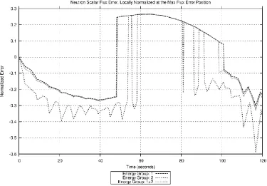
Figure 49: Maximum flux error, 120 second transient, normal beta values, 0.002 second projection operator set. ...60

(9)

vii

Figure 53: Maximum flux error, 2 second transient, normal beta values, high

frequency 0.05 second projection operator set. ...64

Figure 54: Hot-spot flux error, 2 second transient, normal beta values, high frequency 0.05 second projection operator set. ...64

Figure 55: Maximum flux error, 120 second transient, normal beta values, high

Figure 56: Hot-spot flux error, 120 second transient, normal beta values, high

Figure 57: RMS flux error, 2 second transient, 0.002 second projection operator set, update at 1 second, original restart parameters: (0.001 second time-steps). ...66

Figure 58: RMS flux error, 2 second transient, 0.05 second projection operator set, update at 1 second, original restart parameters: (0.001 second time-steps). ...67

Figure 59: RMS flux error, 120 second transient, 0.002 second projection operator set, update at 60 seconds, original restart parameters: (0.01 second time-steps). ...67

Figure 60: RMS flux error, 120 second transient, 0.05 second projection operator set, update at 60 seconds, original restart parameters: (0.01 second time-steps). ...68

Figure 61: RMS flux error, 2 second transient, update at 1 second, 0.01 time-step for annealing and operator production. ...69

Figure 62: RMS flux error, 120 second transient, update at 60 seconds, 0.05 second annealing time-step. ...69

Figure 63: RMS flux error, 2 second transient, update at 1 second, 0.001 second

operator production time-step ...71

Figure 64: RMS flux error, 2 second transient, update at 1 second, 0.002 second

operator production time-step. ...71

Figure 65: RMS flux error, 2 second transient, update at 1 second, doubled projection operator frequency. ...72

Figure 66: Maximum flux error, 2 second transient, update at 1 second, original

projection operator frequency. ...73

Figure 67: Maximum flux error, 2 second transient, update at 1 second, doubled

projection operator frequency. ...73

Figure 68: Maximum flux error, 120 second transient, update at 1 second, original projection operator frequency. ...74

Figure 69: Maximum flux error, 120 second transient, update at 1 second, doubled projection operator frequency. ...74

Figure 70: Flux shape, 2 second transient, rods ½ inserted. ...76

Figure 71: Normalized flux shape error, 2 second transient, 0.002 lo-fi, rods 4/5

(10)

viii

inserted. ...78

Figure 73: Normalized flux shape error, 120 second transient, 0.002 lo-fi, rods 4/5 inserted. ...79

Figure 74: Normalized flux shape error, 120 second transient, 0.05 lo-fi, rods 4/5 inserted. ...80

Figure 75: Normalized precursor delta, 2 second transient, rods 4/5 inserted. ...81

Figure 76: Normalized precursor delta, 120 second transient, rods 4/5 inserted. ...82

Figure 77: Normalized delayed neutron shape delta, 2 second transient, rods 4/5 inserted. ...83

Figure 78: Normalized delayed neutron shape delta, 120 second transient, rods 4/5 inserted. ...84

Figure 79: Power oscillations following step rod and boron decreases, 0.01 second time-step, 1817.30ppm final boron. ...87

Figure 80: Power oscillations following step rod and boron decreases, 0.01 second time-step, 1817.40ppm final boron. ...87

Figure 81: Power oscillations following step rod and boron decreases, 0.01 second time-step, 1817.40ppm final boron, doubled velocity. ...88

Figure 82: Power oscillations following step rod and boron decreases, 0.1 second time-step, 1817.40ppm final boron. ...88

Figure 83: Power oscillations following step rod and boron decreases, 0.1 second time-step, 1817.40ppm final boron, doubled velocity. ...89

Figure 84: Power oscillations following step rod and boron decreases, 0.01 second time-step, 1817.445ppm final boron, normal vs. suppressed betas, 1817.43ppm fixed boron. ...89

Figure 85: Power oscillations following step rod and boron decreases, 0.01 second time-step, 1817.445ppm final boron, 0.1 second ramp reactivity change. ...90

Figure 86: Steady state radial flux shape at various axial heights in the core with bank 9 control rods fully inserted. ...91

Figure 87: Normalized difference in radial flux shape at various axial heights at 0.02 seconds versus 1 seconds. ...92

Figure 88: Normalized difference in radial flux shape at various axial heights at 0.02 seconds versus 1000 seconds. ...93

Figure 89: Normalized difference in radial flux shape, including non-fueled regions, at various axial heights at 0.02 seconds versus 1000 seconds. ...94

Figure 90: Normalized difference in radial delayed neutron production distribution, at various axial heights at 0.02 seconds versus 1 second. ...95

Figure 91: Normalized difference in radial delayed neutron production distribution, at various axial heights at 0.02 seconds versus 1000 seconds. ...96

Figure 92: 2 second rod withdrawal transient maximum flux error, 0.05 second

(11)

ix

Figure 93: 2 second rod withdrawal transient RMS flux error, 0.05 second projection operator set. ... 106

Figure 94: 2 second rod withdrawal transient maximum precursor error, 0.05 second projection operator set. ... 107

Figure 95: 2 second rod withdrawal transient RMS precursor error, 0.05 second

projection operator set. ... 107

Figure 96: Maximum DNP error, 2 second transient, normal beta values, high

frequency 0.05 second projection operator set. ... 108

Figure 97: RMS precursor error, 2 second transient, normal beta values, high

Figure 98: Maximum DNP error, 120 second transient, normal beta values, high frequency 0.05 second projection operator set. ... 109

Figure 99: RMS precursor error, 120 second transient, normal beta values, high

inserted. ... 110

Figure 101: Normalized flux shape error, 2 second transient, 0.05 lo-fi, rods ½

inserted. ... 110

Figure 102: Normalized flux shape error, 2 second transient, 0.05 lo-fi, rods fully inserted. ... 111

Figure 103: Normalized flux shape error, 120 second transient, 0.05 lo-fi, rods 1/5 inserted. ... 111

Figure 104: Normalized flux shape error, 120 second transient, 0.05 lo-fi, rods ½ inserted. ... 112

Figure 105: Normalized flux shape error, 120 second transient, 0.05 lo-fi, rods fully inserted. ... 112

Figure 106: Normalized delayed neutron shape delta, 2 second transient, rods 1/5 inserted. ... 113

Figure 107: Normalized delayed neutron shape delta, 2 second transient, rods ½ inserted. ... 113

Figure 108: Normalized delayed neutron shape delta, 2 second transient, rods fully inserted. ... 114

Figure 109: Normalized delayed neutron shape delta, 120 second transient, rods 1/5 inserted. ... 114

Figure 110: Normalized delayed neutron shape delta, 120 second transient, rods ½ inserted. ... 115

Figure 111: Normalized delayed neutron shape delta, 120 second transient, rods fully inserted. ... 115

Figure 112: Normalized difference in radial flux shape, including non-fueled regions, at various axial heights at 500 seconds versus 1000 seconds.. ... 116

(12)

1

1. Introduction

Designing the core of a nuclear power reactor is an intricate process. There are many requirements that the reactor core must meet, including safety limits for all probable transients. In order to ensure that the reactor can be operated safely, it is important to be able to predict the behavior of the core. Mathematical models are employed to assist in this process as the mechanisms which affect reactor behavior are challengingly complex. While the solution to some mathematical models of reactor behavior can be approximated, and a very few solved using analytical methods, real reactor behavior is best predicted by computer codes that use numerical methods to solve the

mathematical models. Due to the significant variance in relevant timescales, physical dimension, and other properties involved in modeling the behavior of a reactor, the computational cost can be quite high, depending on the desired accuracy and complexity of the model. There are numerous available techniques to reduce the computational burden of reactor modeling, however, there is still opportunity to do more.

1.1 Overview

In an effort to enhance simulation capabilities while at the same time minimizing computational burden, multi-fidelity approaches have been proposed. Often these approaches are used in studies of risk analysis, and consist of many low-fidelity

simulations which pinpoint scenarios which require higher accuracy and thus impose a greater computation cost. Another approach sometimes used is an adaptive mesh refinement (AMR) technique, which is used to vary the resolution of numerical schemes used within a simulation model. For most advanced simulations the associated

(13)

2 intention of combining a low-fidelity and a higher-fidelity model in such a way as to take advantage of the benefits of each. This is done by running the low-fidelity

simulation until an error criteria is reached and improved accuracy is needed, at which point the simulation switches to high-fidelity simulation, hopefully reducing the error and subsequently returning to the low-fidelity simulation. For the purpose of the analysis here, various direct comparisons of the high-fidelity and low-fidelity solutions are used. They are described in Chapter 2. Ideally, the high-fidelity solution would not need to fully compute, as that would make the method redundant. For this purpose, the eventual goal of the AMoR approach is to use an adjoint based method to perform uncertainty quantification for the error prediction.

1.2 Theoretical basis

Most neutron behavior modeling solutions and codes are based on the neutron transport equation. [4]

1 𝑣(𝐸) 𝜕 𝜕𝑡𝜓(𝑟⃑, 𝐸, Ω̂, 𝑡) + Ω̂ ∙ ∇𝜓(𝑟⃑, 𝐸, Ω̂, 𝑡) +Σ𝑡(𝑟⃑, 𝐸, 𝑡)𝜓(𝑟⃑, 𝐸, Ω̂, 𝑡) = ∫ 𝑑Ω̂′ 4π ∫ 𝑑𝐸∞ ′ 0 Σ𝑠(𝑟⃑, 𝐸′ → 𝐸, Ω̂′∙ Ω̂, 𝑡)𝜓(𝑟⃑, 𝐸′, Ω̂′, 𝑡)

+𝜒(𝑟⃑, E, 𝑡) 4𝜋 ∫ 𝑑Ω̂′

4π ∫ 𝑑𝐸∞ ′ 0 𝜈_𝑓(𝑟⃑, 𝐸′_{, 𝑡)}_Σ 𝑓(𝑟⃑, 𝐸′, 𝑡)𝜓(𝑟⃑, 𝐸′, Ω̂′, 𝑡) + 𝑄(𝑟⃑, 𝐸, Ω̂, 𝑡) (1.1)

(14)

3 interactions. The external neutron source term, 𝑄(𝑟⃑, 𝐸, Ω̂, 𝑡), may also vary with

position, neutron energy, travel direction, and time.

The delayed fission neutron source term is not explicitly included in the form of the equation shown here. The neutron transport equation is based on the Boltzmann equation and, while it unambiguously represents the behavior of neutrons in time and space, it is extremely difficult to solve for all but the simplest theoretical situations. There are many different approaches to applying the neutron transport equation; one of the most common is to derive and use approximations of it that are sufficiently accurate for practical applications. A commonly used approximation is the multi-group diffusion equation, a principle tool for modeling nuclear reactors.[4]

1 𝑣(𝐸) 𝜕 𝜕𝑡𝜙(𝑟⃑, 𝐸, 𝑡) − ∇ ∙ 𝐷(𝑟⃑, 𝐸, 𝑡)∇𝜙(𝑟⃑, 𝐸, 𝑡) +Σ𝑡(𝑟⃑, 𝐸, 𝑡)𝜙(𝑟⃑, 𝐸, 𝑡) = ∫ 𝑑𝐸∞ ′ 0 Σ_𝑠(𝑟⃑, 𝐸′_{→ 𝐸, 𝑡)𝜙(𝑟⃑, 𝐸, 𝑡)} + 𝜒(𝑟⃑, 𝐸, 𝑡) ∫ 𝑑𝐸∞ ′

0 𝜈𝑓(𝑟⃑, 𝐸′, 𝑡)Σ𝑓(𝑟⃑, E′, 𝑡)𝜓(𝑟⃑, 𝐸′, 𝑡) + 𝑄(𝑟⃑, 𝐸, 𝑡)

(1.2)

(15)

4

1.3 NESTLE

The high-fidelity code employed here was NESTLE, standing for Nodal Eigenvalue, Steady-state, Transient, Le core Evaluator. NESTLE is a few-group neutron diffusion equation solver utilizing the nodal expansion method. The code was primarily written in FORTRAN 77; code used in this project also employs subroutines written in

FORTRAN 90. NESTLE’s capabilities include solving the eigenvalue (criticality), eigenvalue adjoint, external fixed-source steady-state, or external fixed-source or eigenvalue initiated transient problems. The code supports utilization of two or four neutron energy groups, though only two groups were employed in this endeavor. It is capable of modeling Cartesian and Hexagonal geometries and three, two, or one spatial dimensions. While the code has thermal-hydraulic feedback capability, it was turned off for the purpose of simplifying the investigations conducted here. NESTLE has many additional features not used in this study [2]. One of NESTLE’s features that is utilized is the restart capability. NESTLE can resume a transient simulation after being

stopped using saved data from the end of the previous run.

All non-restart transient runs begin with a steady-state initialization, wherein NESTLE numerically solves the multi-group steady-state diffusion equation in eigenvalue form, shown here with spatial dependency suppressed.

−∇ ∙ 𝐷_𝑔∇𝜙_𝑔+Σ_𝑡𝑔𝜙_𝑔= ∑ Σ_𝑠𝑔𝑔′

𝐺

𝑔′₌₁

𝜙_𝑔′+𝜒𝑔

𝑘 ∑ 𝜈𝑔′

𝐺

𝑔′₌₁

Σ_𝑓𝑔′𝜙_𝑔′

(1.3)

Spatial discretization is achieved using the finite difference method. Nodal Expansion Method (NEM) is used to modify the diffusion coupling coefficients in order to correct the errors introduced by the finite difference method and material homogenization. Transient runs are treated similarly, with the addition of time and delayed neutrons as shown in Eq. (1.4) and (1.5), with time and spatial dependencies depressed.

1 𝑣𝑔

𝜕𝜙𝑔

𝜕𝑡 = 𝛻 ∙ 𝐷𝑔𝛻𝜙𝑔−Σ𝑡𝑔𝜙𝑔+ ∑Σ𝑠𝑔𝑔′ 𝐺

𝑔′₌₁

𝜙𝑔′+ (1 − 𝛽)𝜒𝑔(𝑃)∑ 𝜈𝑔′ 𝐺

𝑔′₌₁

(16)

5

𝐶𝑖 is the concentration of delayed neutron precursor (DNP) group i, 𝜆𝑖is the DNP group

decay constant, and 𝛽_𝑖 is the fraction of all fission neutrons emitted per fission in a DNP group while 𝛽 is the fraction of all fission neutrons that are born delayed, or the sum of 𝛽_𝑖.

1.4 Point Kinetics and Quasi-static Method

A further simplification of the diffusion equation, the point reactor kinetics model assumes that the spatial flux shape does not change with time. Assuming one neutron energy group, the flux and precursor distributions can be factorized, or treated as having independent amplitude and spatial dependence:

𝜙(𝑟⃑, 𝑡) = 𝑣𝑛(𝑡)𝜓(𝑟⃑)

𝐶𝑖(𝑟⃑, 𝑡) = 𝐶𝑖(𝑡)𝜓(𝑟⃑)

(1.6)

Substituting these expressions into the one-group diffusion equation along with an expression for the prompt neutron lifetime 𝑙 provides the point reactor kinetics equations (PKE) shown here with six delayed neutron precursor groups:

𝑑𝑛(𝑡) 𝑑𝑡 =

𝑘(1 − 𝛽) − 1

𝑙 𝑛(𝑡) + ∑ 𝜆𝑖𝐶𝑖(𝑡) 6 𝑖=1 𝜕𝐶𝑖(𝑡) 𝜕𝑡 = 𝛽𝑖 𝑘

𝑙𝑛(𝑡) − 𝜆𝑖𝐶𝑖 𝑓𝑜𝑟 𝑖 = 1, … ,6

(1.7)

Most often, reactivity is used in place of the multiplication factor,

𝜌 ≡𝑘 − 1

𝑘 . (1.8)

This model is typically used to simulate average behavior of a reactor during a

transient [4]. Even though the assumption of non-variant flux shape may be incorrect, and

𝜕𝐶𝑖

𝜕𝑡 = 𝛽𝑖∑ 𝜈𝑔

𝐺

𝑔=1

(17)

6 the core average values determined by the point kinetics model can be quite accurate, due in part to improvements from the quasi-static approach.

The quasi-static approach of reactor kinetics was introduced in 1958 by Allan Henry as a modification of the original point kinetics method. He proposed that, rather than treating the spatial dependence or ‘shape’ of neutron flux as constant, it would instead change gradually with time.

𝜙(𝑟⃑, 𝑡) = 𝑣𝑛(𝑡)𝜓(𝑟⃑, 𝑡) (1.9)

The purpose of the quasi-static method was to improve the point kinetics parameters (k,l), which do vary with flux shape and thus time [3]. The method assumes that the timescale over which flux shape changes and perceptibly affects the point kinetic parameters (PKP) is relatively long, thus it permits recalculating them at longer time intervals than the amplitude time-step intervals. Two main techniques were developed for improving the PKP, called the ‘Improved Quasi-static Method’ (IQM), and the ‘Predictor-Corrector Quasi-static Method’ (PCQM) [3].

1.5 PKE-solver

A point kinetics equation solver is used as the basis of the low-fidelity method. It solves equation (1.7) for core average neutron density using reactivity and other point kinetic parameters calculated beforehand using a point kinetics parameters routine that was added to NESTLE. The defining equations for the PKP have been derived using a variational technique. Using forward and adjoint steady state flux calculated by NESTLE, a perturbation in reactivity is calculated as

∆𝜌 =̃−〈𝜙

†_{, 𝛿Σ} 𝑎𝜙〉

〈𝜙†_{, F𝜙〉} , (1.10)

where 𝜙†_{is the adjoint flux,}_𝛿Σ

𝑎 is the source of the perturbation, F𝜙 represents the

(18)

7 RAMBO User’s Manual [6]. It is significant to note that the parameters calculated in this method differ from straight volume-averaged values as they are adjoint-weighted. The point kinetic parameters are calculated at multiple representative ‘times’, or rod heights, to capture the effect of changing flux shape on the parameters. They only have to be recalculated if changes are made to basic core data or a different source of

reactivity change were to be modeled.

1.6 Adaptive Model Refinement

The low-fidelity model for AMoR uses the improved point kinetics results and includes a separate prediction of the flux shape over time to produce a three dimensional solution that can be directly compared to a full high-fidelity solution. AMoR takes the average neutron density produced by PKE and projects it to three dimensions via multiplication by projection operators which, in combination, relate the mono-energetic core average neutron density to energy group and spatially dependent flux. The

(19)

8

2. Methodology

The reactor core being simulated for this research was a quarter core slice of a

Westinghouse 4-loop, 3,311 MWt, PWR. The geometric and material inputs, as well as the cross-section data were from a sample data set representing Cycle 13 of McGuire Nuclear Station, Unit 1. It was modeled using two neutron energy groups and six delayed neutron precursor groups. Xenon and Samarium were suppressed and thermal-hydraulic feedback was turned off in order to reduce simulation complexity and allow clearer results.

2.1 Projection Operator Production

In order to produce a three-dimensional model using the PKE-solver, a prediction of the flux shape and energy distribution is needed. The factors used to transform the mono-energetic, average neutron density into a three-dimensional, two-group flux are called projection operators. The projection operators are generated by NESTLE prior to running the low-fidelity solution and can be produced in different manners, discussed further in Chapter 3. In all variations the method of calculating the projection

operators is the same. Primary values NESTLE calculates include scalar flux,

𝜙(𝑟⃑, 𝐸, 𝑡) → 𝜙_𝑔,𝑚(𝑡), (2.1)

precursor group concentration,

𝐶_𝑖(𝑟⃑, 𝑡) → 𝐶𝑖,𝑚(𝑡), (2.2)

and neutron velocity,

𝑣(𝑟⃑, 𝐸, 𝑡) → 𝑣_𝑔,𝑚(𝑡), (2.3)

(20)

9 projection operators from these primary values. Following are the equations used to calculate the projection operators, starting with the neutron density distribution,

𝑛𝑔,𝑚(𝑡) =

𝜙_𝑔,𝑚(𝑡)

𝑣𝑔,𝑚(𝑡) , (2.4)

from which the volume averaged neutron density is calculated,

〈𝑛(𝑡)〉 =∫ 𝑑𝑉𝑉 ∫ 𝑑𝐸 ∞

0 𝑛(𝑟⃑, 𝐸, 𝑡)

∫ 𝑑𝑉_𝑉 =

∑𝑀𝑚=1∑2𝑔=1𝑛𝑔,𝑚(𝑡)𝑉𝑚

∑𝑀𝑚=1𝑉𝑚

. (2.5)

Two more intermediaries in developing the projection operators are the energy dependent volume averaged scalar flux,

〈𝜙𝑔(𝑡)〉 =

∫ 𝑑𝑉_𝑉 ∫𝐸𝑔 𝑑𝐸

𝐸𝑔−1 𝜙(𝑟⃑, 𝐸, 𝑡)

∫ 𝑑𝑉_𝑉 =

∑𝑀 𝜙_𝑔,𝑚(𝑡)

𝑚=1 𝑉𝑚

∑𝑀 𝑉_𝑚

𝑚=1

, (2.6)

and the volume averaged scalar flux,

〈𝜙(𝑡)〉 =∫ 𝑑𝑉𝑉 ∫ 𝑑𝐸

∞

0 𝜙(𝑟⃑, 𝐸, 𝑡)

∫ 𝑑𝑉_𝑉 =

∑𝑀𝑚=1∑2𝑔=1𝜙𝑔,𝑚(𝑡)𝑉𝑚

∑𝑀𝑚=1𝑉𝑚

, (2.7)

from which the flux energy partition function is calculated:

〈𝑓_𝑔(𝜙)(𝑡)〉 =〈𝜙𝑔(𝑡)〉

〈𝜙(𝑡)〉 . (2.8)

The volume averaged neutron velocity is calculated as,

〈𝑣(𝑡)〉 =〈𝜙(𝑡)〉

〈𝑛(𝑡)〉 . (2.9)

(21)

10

〈𝑛̅(𝑡)〉 = 〈𝑛(𝑡)〉

〈𝑛(0)〉 . (2.10)

Initial volume averaged neutron density, 〈𝑛(0)〉, is therefore a critical parameter for employing the projection operators. All volume averaged values are only averaged over the fueled nodes, rather than the entirety of the geometric core, as the PKE-Solver is only capable of approximating the region of the core containing fuel.

Once the energy dependence of the projection is set, the average-normalized spatial distribution, or shape-factors can be calculated. The scalar flux shape-factor is calculated as,

𝑆_𝑔,𝑚(𝜙)(𝑡) =𝜙𝑔,𝑚(𝑡)

〈𝜙𝑔(𝑡)〉 . (2.11)

Through these calculations the flux is factorized from a 3-D form into an amplitude-shape form, represented as,

𝜙_𝑔,𝑚(𝑡) = 𝑆_𝑔,𝑚(𝜙)(𝑡) 〈𝑓_𝑔(𝜙)(𝑡)〉 〈𝑣(𝑡)〉〈𝑛̅(𝑡)〉〈𝑛(0)〉 . (2.12)

In the original form of the AMoR method, the low-fidelity delayed neutron precursor concentration distribution was predicted using projection operators as well. The precursor related projection factors are still calculated, although they are no longer used for that purpose. Volume averaged precursor group concentration is calculated as,

〈𝐶𝑖(𝑡)〉 =

∫ 𝐶_𝑉 𝑖(𝑟⃑, 𝑡)𝑑𝑉

∫ 𝑑𝑉_𝑉 =

∑𝑀𝑚=1𝐶𝑖,𝑚(𝑡)𝑉𝑚

∑𝑀 𝑉_𝑚

𝑚=1

, (2.13)

from which the precursor group concentration shape-factor is calculated,

𝑆_𝑖,𝑚(𝐶)(𝑡) =𝐶𝑖,𝑚(𝑡)

(22)

11

2.2 Low-Fidelity Projection and Precursor prediction

The 3-D, energy dependent low-fidelity projected flux approximation is calculated as,

𝜙̃𝑔,𝑚(𝑡) = 𝑆𝑔,𝑚(𝜙)(𝑡) 〈𝑓𝑔(𝜙)(𝑡)〉 〈𝑣(𝑡)〉〈𝑛̃(𝑡)〉〈𝑛(0)〉 , (2.15)

where the normalized volume averaged neutron density from the NESTLE projection-operator producing run is replaced by the approximate normalized volume averaged neutron density calculated by the PKE-solver. The projection operators are matched up to the appropriate low-fidelity neutron density corresponding to the concurrent rod position; for this reason all projection operator related files are indexed by rod position. When the current rod position of the low-fidelity simulation does not directly

correspond to a set of files, the projection operator values are approximated using linear interpolation. This linear interpolation impacts the accuracy of the low-fidelity model; the specifics of this will be discussed in results section 3.3.4.

In the original method, a low-fidelity precursor concentration was calculated using an analogous projection,

𝐶̃𝑖,𝑚(𝑡) = 𝑆𝑖,𝑚(𝐶)(𝑡) 〈𝐶̃𝑖(𝑡)〉 〈𝐶𝑖(0)〉 . (2.16)

In order to improve model accuracy, the projection method was replaced in the low-fidelity solution with a direct calculation of a delayed neutron precursor concentration from the low-fidelity projected flux. This set of equations is precisely the same as those used in the high-fidelity NESTLE diffusion model, however they are not significantly more computationally burdensome than the projection method, as they do not involve the solution of coupled algebraic equations. The precursor equation, Eq. (1.5), is solved utilizing the Integrating Factor method, giving,

𝐶_𝑖(𝑡𝑛) = 𝐶𝑖(𝑡𝑛−1)𝑒−𝜆𝑖∆𝑡𝑛+ 𝛽𝑖 ∫ ∑ 𝜈𝑔 𝐺

𝑔=1

𝛴_𝑓𝑔𝜙_𝑔(𝑡′)

𝑡𝑛

𝑡𝑛−1

𝑒−𝜆𝑖(𝑡𝑛−𝑡′)𝑑𝑡′, (2.17)

where the current time-step’s precursors depend on the previous precursor

(23)

12 fission source between time-steps, this equation is approximated for numerical solution as,

𝐶_𝑖(𝑡𝑛) = 𝐶𝑖(𝑡𝑛−1)𝑒−𝜆𝑖∆𝑡𝑛+ 𝐹𝑖𝑛

0 _{∑ 𝜈}

𝑔 𝐺

𝑔=1

𝛴_𝑓𝑔𝜙_𝑔(𝑡𝑛−1) + 𝐹𝑖𝑛

1 _{∑ 𝜈}

𝑔 𝐺

𝑔=1

𝛴_𝑓𝑔𝜙_𝑔(𝑡𝑛), (2.18)

where

𝐹_𝑖1_𝑛 = 𝛽𝑖

𝜆_𝑖∆𝑡_𝑛[∆𝑡𝑛− 1

𝜆_𝑖(1 − 𝑒−𝜆𝑖∆𝑡𝑛)] (2.19)

and

𝐹_𝑖0_𝑛 _{= −𝐹} 𝑖𝑛

1 ₊𝛽𝑖

𝜆_𝑖[(1 − 𝑒−𝜆𝑖∆𝑡𝑛)] . (2.20)

[2]. The relative accuracy of directly calculated and projected precursor concentrations is discussed in section 3.2. This calculation of the delayed neutron precursor

concentration is not fed back in to the low-fidelity solution as the PKE-solver already has a similarly solved core-average delayed neutron precursor concentration it uses, which is calibrated to work with the adjoint-weighted PKP values.

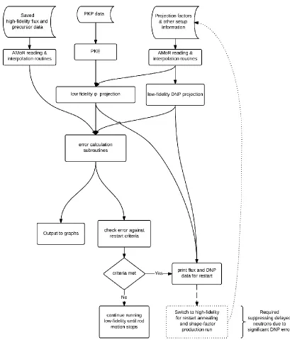
2.3 Hereditary AMoR Setup

(24)

13

(25)

14 In the original AMoR setup, all NESTLE and PKE-solver simulations were run

separately. Figure 1 shows the runs required for initial setup of a new sample

transient. Subsequent transients will reuse the saved data unless essential parameters are altered.

(26)

15 Following a NESTLE run, pertinent data which had been saved by AMoR routines during the transient could be transferred to and read in by the AMoR routines associated with producing the low-fidelity solution, as well as error computations, as illustrated in Figure 2.

One limitation of this code setup is that it requires saving information from the high-fidelity NESTLE solution to be used for comparison to the low-high-fidelity solution. Using saved data requires either recording information for every relevant time step, a significant amount of data, or interpolating between a set of saved points.

Interpolating between saved points corresponding to rod position, as in the low-fidelity interpolation scheme, was selected to minimize the amount of data that had to be stored and transferred. While this scheme gives sufficient accuracy for most situations, it exhibits a minor flaw relating to subsequent DNP concentration calculations as discussed further in results section 3.2.2.

In the current system, the projection operators used in the low-fidelity solution must be produced by a NESTLE run and indexed by rod position. There are several choices available for NESTLE runs that will provide a reasonably accurate low-fidelity solution to a given rod insertion transient. One such option is to produce a library of steady state based projection operators corresponding to a pre-selected number of different rod positions. The accuracy and appropriateness of the steady state library was explored as part of Sterling Satterfield’s work [1]. Another option is to use a rapid rod insertion to model the prompt neutron behavior during a longer rod insertion transient, as it is the shorter transient will have a commensurately shorter run-time. This method was initially explored as part of Satterfield’s work [1], and the one selected for further evaluation here.

In the current setup, as well, the AMoR routines that save the projection operators are run parallel to those that save the flux and DNP concentration of the high-fidelity solution. This allows the corresponding shape-factor and energy dependence

(27)

16

2.4 Active Switching Concept & Methodology

Depending on preset error criteria, at some point during a given transient there will be a need to switch from the low-fidelity model to the high fidelity model in order to reduce the error. Once the error of the low-fidelity model grows too large, the flux and precursor information from preceding time steps are fed, along with rod position, back into the high-fidelity model. This is done by printing out the relevant low-fidelity data, pausing the low-fidelity run, and performing a high-fidelity NESTLE restart which uses the low-fidelity flux and precursor data as initial conditions with the expectation that the restarted high-fidelity run will “anneal” out the error. This is immediately followed by a simulation of a rapid transient which models the remainder of the rod motion transient, producing updated projection operators. The low-fidelity run is

resumed and the new projection operators are used for the remainder of the low-fidelity run, or until the error again grows too large. The “annealing” process relies on the use of low-fidelity data from a prior time-step rather than the one which triggers the restart. The historical low-fidelity data are input into the NESTLE code as initial conditions from which a transient using small time increments is executed up to the current time-step, reducing the error each time the flux and precursor data are fed through the high-fidelity diffusion calculations. This is possible due to the constant relationship between production and loss terms. A mathematical argument for this is contained in Sterling Satterfield’s work [1].

(28)

17 the need for this makeshift fix was removed by changing the method by which the low-fidelity DNP concentration was determined. The projection method of DNP calculation, represented by Eq. (2.16) was replaced by direct calculation from low-fidelity flux as previously shown in Eqs. (2.18), (2.19), and (2.20). As will be discussed further in section 3.2, this significantly increased the accuracy of the low-fidelity DNP concentration prediction, thus permanently removing that hindrance to the active switching.

2.5 Hereditary Error Metrics

Many of the error analysis tools used in this report were developed by Sterling

Satterfield [1] as part of the initial technique verification. Following is a brief summary of the error metrics utilized again here. Key error metrics of interest were ones that tended to demonstrate the largest magnitude of error, and those that most directly exhibited the success or failure of an attempted method modification. The error metric which consistently showed the largest error, which would trigger switching criteria, and excluding precursors calculated using the original projection method, was locally normalized flux error,

𝜀_{𝑓𝑙𝑢𝑥.𝑙𝑜𝑐𝑎𝑙,𝑔}=𝜙𝑔,𝑚∗(𝑡) − 𝜙̃𝑔,𝑚∗(𝑡)

𝜙𝑔,𝑚∗(𝑡) , (2.21)

at the maximum flux error position:

𝑚∗_{= arg max} 𝑚

|𝜙𝑔,𝑚(𝑡) − 𝜙̃𝑔,𝑚(𝑡)|

𝜙_𝑔,𝑚(𝑡) . (2.22)

The largest flux errors in a transient are found near the rod tip as it moves through the core. As the largest relative flux error in the core is likely to not properly represent an overall picture of the core flux error or locations of particular interest such as hot spots, a better metric for that purpose is the average normalized flux error,

𝜀_{𝑓𝑙𝑢𝑥.𝑎𝑣𝑔,𝑔} =𝜙𝑔,𝑚∗(𝑡) − 𝜙̃𝑔,𝑚∗(𝑡)

(29)

18 at the maximum flux position:

𝑚∗_{= arg max}

𝑚 |𝜙𝑔,𝑚(𝑡)| . (2.24)

The metrics for precursor concentration error are formulated in the same manner. In several instances it was desired to examine the error of the shape-factors

specifically, as these were determined to be the largest contributor to the overall error; this is discussed in Section 3.3. Recalling the formulation of the projected flux in section 2.2, removing the other projection operators allows calculation of locally or average normalized flux-shape errors,

𝜀_{𝑓𝑙𝑢𝑥⋅𝑠ℎ𝑎𝑝𝑒.𝑙𝑜𝑐𝑎𝑙,𝑔}=𝑆𝑔,𝑚∗ (𝜙) _{(𝑡) − 𝑆̃} 𝑔,𝑚(𝜙)∗(𝑡) 𝑆_𝑔,𝑚(𝜙)∗(𝑡) , (2.25) 𝜀𝑓𝑙𝑢𝑥⋅𝑠ℎ𝑎𝑝𝑒.𝑎𝑣𝑔,𝑔= 𝑆_𝑔,𝑚(𝜙)∗(𝑡) − 𝑆̃_𝑔,𝑚(𝜙)∗(𝑡) 〈𝑆_𝑔(𝜙)(𝑡)〉 , (2.26)

at the maximum flux or maximum flux error positions as described in equations (2.22) and (2.24).

The best representation of the overall core-wide flux error is the volume weighted L-2 norm or RMS error of the flux,

𝜀_{2,𝑓𝑙𝑢𝑥.𝑡𝑜𝑡𝑎𝑙}= √

∑𝑀 [(𝜙_𝑚(𝑡) − 𝜙̃_𝑚(𝑡))2∆𝑧_𝑚]

𝑚=1

𝑀_𝑥𝑦𝑍

1

〈𝜙(𝑡)〉 , (2.27)

where

𝑍 = 1

𝑀𝑥𝑦 ∑ ∆𝑧𝑚 𝑀 𝑚=1 , (2.28) and 𝑀_𝑥𝑦= 𝑀

𝑀_𝑧. (2.29)

Z, total height of the core, and ∆𝑧𝑚, height of the mth node, are used in place of core

(30)

19 height of Z-planes varies. 𝑀_𝑥𝑦 is the number of nodes in a single XY-plane, 𝑀_𝑧 is the number of Z-planes, and M is still the total number of nodes.

Normalized volume averaged neutron density,

〈𝑛̅(𝑡)〉 = 〈𝑛(𝑡)〉

〈𝑛(0)〉 , (2.30)

and normalized volume averaged precursor group concentration,

〈𝐶̅𝑖(𝑡)〉 =

〈𝐶𝑖(𝑡)〉

〈𝐶𝑖(0)〉 , (2.31)

were used as measures of method stability in specific instances.

2.6 Additional Error Metrics

In addition to the error metrics originally developed and used by Satterfield [1], two new error analysis techniques were introduced. The first was to look at the Root Mean Square (RMS) error in the flux shape, which was formulated as,

𝜀_{𝑅𝑀𝑆,𝑓𝑙𝑢𝑥⋅𝑠ℎ𝑎𝑝𝑒,𝑔}=√

∑𝑀 [(𝑆_𝑔,𝑚(𝜙)(𝑡) − 𝑆̃_𝑔,𝑚(𝜙)(𝑡))2∆𝑧_𝑚]

𝑚=1

𝑀_𝑥𝑦𝑍 .

(2.32)

This metric was added to assist in evaluating the overall core-wide errors, as a representation of the shape-factor specific average error. In general, the RMS flux shape error and the local flux-shape errors behave similarly.

(31)

20 The third additional error metric is intended to eventually be used to bypass the need to calculate a full high-fidelity solution. For this metric, the low-fidelity flux is

employed in combination with generalized perturbation theory (GPT) adjoint flux to produce error responses which indicate the relative error in a given core location at a given point in time. The time and core location of interest are predefined using a response function, 𝑓. Starting with the high-fidelity flux, 𝜙, with A being the high fidelity operator, and the low-fidelity flux, 𝜙,̃ with 𝐴̃ being the low-fidelity operator, then

𝐴𝜙 = 0, 𝐴̃𝜙̃ = 0, & Δ𝜙 = 𝜙̃ − 𝜙. (2.33) The residual is calculated as

𝑟 = 𝐴𝜙̃. (2.34)

The error response is defined as

𝑅 = 〈𝑓, Δ𝜙〉. (2.35) The adjoint solution, Ψ∗_,_{measures the importance of neutrons in regards to the}

response function [7]. When combined with the adjoint operator, 𝐴∗_,_{it reproduces the}

response function.

𝐴∗_Ψ∗_{= 𝑓.} _(2.36)

The adjoint operator is defined as

〈ϕ∗_{, 𝐴𝜙〉 = 〈𝐴}∗_ϕ∗_{, 𝜙〉.} _(2.37)

The error response measured by eq. (2.35) can also be produced as

𝑅 = 〈Ψ∗_{, 𝑟〉,} _(2.38)

since,

𝑅 = 〈Ψ∗_{, 𝑟〉 = 〈Ψ}∗_{, 𝐴𝜙̃〉 = 〈Ψ}∗_{, 𝐴(𝜙̃ − 𝜙)〉 = 〈𝐴}∗_Ψ∗_{, 𝜙̃ − 𝜙〉 = 〈𝑓, Δ𝜙〉.} _(2.39)

The error response calculated using the adjoint method would hopefully permit measuring the relative error in the low-fidelity solution without requiring the high-fidelity forward solution for comparison. At this time the method is not fully

(32)

21

(33)

22

3. Results

This project phase was focused on two main activities. The first was to finish the development and evaluation of the AMoR method and begin the process of combining all aspects of AMoR into one code. A copy of NESTLE was modified to have the PKE-Solver encoded within it prior to the initiation of this work. Further work to include production of the low-fidelity solution and error analysis was performed as part of this research, based on AMoR routines developed by Sterling Satterfield. In addition, the modeling capabilities of the PKE-Solver and AMoR were expanded. Satterfield demonstrated that the AMoR model was essentially functional [1]. Section 3.2 of this work describes tasks that were performed to complete the implementation of the low-fidelity model, and the added functionalities in more detail.

The second goal of this research was to find ways to improve the low-fidelity model by reducing the inherent error. This required identifying the specific sources which were contributing to the error. Section 3.3 covers the various efforts to find improvements.

3.1 Test Setup

The simulations were performed on a standard desktop computer running Windows 7 64-bit. The base codes used are NESTLE v5.2.1 [2] and a PKE-Solver. Both codes were modified prior to this project, and further modified in the course of this work, as

described in section 3.2. The codes were compiled, debugged and executed with Microsoft Visual Studios 2012 using the Intel FORTRAN compiler.

(34)

XY-23 planes being represented with 18x18 nodes. The approximately cylindrical core

requires that not all nodes contain core material. The fueled region consists of the inner 26 Z-planes and a specific portion of the XY nodes. Xenon and Samarium were suppressed and thermal-hydraulic feedback was turned off. The simulation employed a constant coolant inlet temperature of 555.50°F and a constant coolant mass flow rate of 1,439,284.5 lb/(ft2_sec).

(35)

24

3.2 The Hybrid Low-Fidelity Model

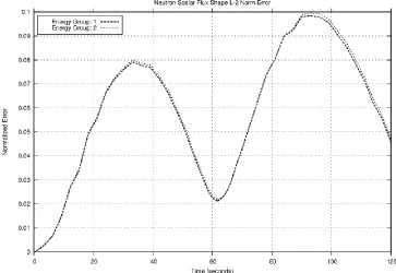
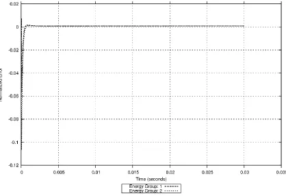
In previous work by Satterfield [1], it was determined that if steady state projection operators were used, for a 2 second rod insertion the largest flux error was near 30%, as seen in Figure 4. The flux error at the maximum flux location reached

approximately 10%, as shown by Figure 5. In all of the cases discussed here, the projected solution is being compared to a high-fidelity solution that is calculated by NESTLE, saved in 40 equidistant snapshots, and interpolated for intermediate values. For the “active model switching” method the projection operators were generated at 20 equidistant points during a rapid insertion transient occurring over 0.002 seconds. Representative flux errors are shown in Figure 6 and Figure 7. While the original rapid-insertion projection operators yielded larger maximum errors, the steady state projection operators yielded larger flux errors at hot-spot locations, which is

undesirable.

(36)

25

Figure 5: Hot-spot flux error for 25 steady-state projection operator sets.

(37)

26

3.2.1 Original Precursor Error

Both sets of projection operators yielded substantial local DNP concentration errors throughout the core with the original method of generating low-fidelity precursor values. For the steady-state projection operators, DNP concentration error reached nearly 70% at its maximum value, as seen in Figure 8. The RMS precursor error, representing core-wide average precursor error, reached over 30% and is shown in Figure 9. For the 0.002 second rapid-insertion projection operator set, DNP

concentration error reached nearly 120% at its absolute maximum value, as seen in Figure 10. The RMS precursor error reached approximately 16%, as shown in Figure 11. The general relationship of the flux and precursor errors for the 120 second rod insertion are comparable to those discussed here for the 2 second rod insertion.

(38)

27

Figure 8: Maximum precursor error for 25 steady-state projection operator sets.

(39)

28

Figure 10: Maximum precursor error for 0.002 second rapid-insertion projection operator sets.

(40)

29

3.2.2 Reducing Precursor Error

The AMoR method is designed to allow transition from a low-fidelity to a high-fidelity simulation and back again. In order for this to work correctly, the low fidelity solution must have sufficient accuracy for the high fidelity portion to render properly. The original low-fidelity projection method did not provide sufficient accuracy in the DNP concentration to allow for the restarts to function properly. In order to test the active switching the previous efforts had included a workaround of artificially suppressing the DNP concentration via setting all beta values to 0.0001. This succeeded as it made the relatively large DNP error mostly irrelevant. In order to enable use of AMoR active switching on a real simulation, the restart capability necessitated improving the accuracy of the low-fidelity DNP concentration. This was done by adding internal calculation of low-fidelity delayed neutron precursor concentration using the projected flux in place of using the original direct projection method for the DNP concentration. This newer approach was designated as a hybrid precursor model as it uses the 3-D precursor equations from NESTLE as described in Section 2. These calculations are straightforward and computationally efficient; they do not significantly impact the overall computational cost of the low-fidelity solution.

Once the precursor calculations were in place, for the set of 0.002 second rapid-insertion projection operators used for a 2 second transient, the maximum DNP

(41)

30

Figure 12: Maximum precursor error for rapid-insertion projection operators hybrid method.

(42)

31 At this point the major contribution to DNP concentration errors should be due to errors in the low-fidelity flux. The precursor errors are now sufficiently small that when the projected flux and precursor information are fed back into the high-fidelity model for a shape-factor update, the resulting updated shape-factors lead to significant overall error reduction as seen in Figure 14. These results show similar error behavior to those produced in active switching when delayed neutrons were suppressed, shown in Figure 15. Since there is still some error in the precursors, it is to be expected that the update on the hybrid solution does not result in quite the same magnitude

improvement as compared to when the precursor values were artificially made

insignificant. The updates were done using restart parameters identical to the original settings used by Satterfield [1]; they are examined more in Section 3.3.5.

(43)

32

(44)

33 Testing to verify that the precursor values were being calculated correctly revealed a non-zero (greater than machine error) minimum precursor error level, even when using flux values imported from the high-fidelity solution. This was determined to be due to regular minor fluctuations (appearing as bumps) in the neutron density calculated within NESTLE over the transient, which cannot be entirely captured by interpolation even with reasonably increased number of data points. Minor differences in flux history between the interpolated high-fidelity flux and the true high-fidelity flux lead to small, but accumulating, differences over time in the precursor values derived from those fluxes. These small fluctuations in neutron density are most likely due to limitations within NESTLE in modeling flux at the node containing the rod-tip.

(45)

34 To clearly see the fluctuations, the difference between a PKE projected flux using high-fidelity data values for the projection, and the true NESTLE flux are plotted against rod position in a representative non-rodded location in Figure 16 and Figure 17.

The tests were repeated in the combined code discussed in section 3.2.3, with continuous transfer of flux values from the high-fidelity solution to the precursor calculations. Delayed neutron precursor calculation results were then found to be off by less than machine error.

(46)

35

3.2.3 New AMoR Layout

As part of continuing work on potential future publication/release of the code as a fully functional package, further modifications were performed to streamline and simplify the code for Adaptive Model Refinement in order to include it as a side capability within NESTLE. A significant portion of the original AMoR code had been set up to handle transfer of data between the separate PKE and NESTLE programs. With PKE and the AMoR functions running within the NESTLE environment, much of this data transfer became unnecessary and the associated subroutines were pared down or removed. After import, the AMoR functions and calls were structured as shown in Figure 18.

(47)

36

(48)

37

3.2.4 Additional Modifications

The original scope of AMoR was to investigate the accuracy of modeling flux and precursors during a rod insertion transient. In order to provide low-fidelity modeling capabilities for a wider variety of transients, the codes and subroutines required

modifications. Capabilities added thus far include modeling a rod withdrawal transient and extending modeling of the low fidelity transient to include times after rod motion has stopped. The low-fidelity solution can also now be used as input to calculate error responses, as described in Section 2.6.

Test results of the rod withdrawal transient appeared to be reasonable. Figure 19 shows the PKE calculated vs. NESTLE calculated average neutron density for a 2 second rod withdrawal transient with 0.5 seconds of subsequent transient shown. Figure 20 and Figure 21 show the maximum and RMS flux errors while Figure 22 and Figure 23 show the corresponding precursor errors. To be consistent with the original rod-insertion tests, a 0.002 second rapid rod withdrawal was used to produce the low-fidelity projection operators for this test.

The rod-withdrawal capability is clearly functional, however, the accuracy of the low-fidelity model is challenged by the rate at which power and average neutron density change. It is clear that there is significant error present in the flux, and especially the DNP concentration. Examining the increasing separation of the high-fidelity and low-fidelity neutron densities as the transient progresses, it is certain that this contributes greatly to the flux error in the latter portions of the transient. Additionally, the

(49)

38

Figure 19: 2 second rod withdrawal transient average neutron density.

(50)

39

Figure 21: 2 second rod withdrawal transient RMS flux error.

(51)

40 During rod motion, the low-fidelity projection operators and high-fidelity solution are read in and interpolated based on rod position. After rod motion ends, the data are switched to a time-based input for the high-fidelity solution. The low-fidelity solution after this point uses the last set of projection operators, as flux shape changes after rod motion ends are expected to be relatively subtle.

When modeling very long transients it was determined that attempts to reduce the frequency of the high-fidelity snapshots lead to significant interpolation errors that overpower all other error sources. Maintaining the original frequency for long follow-up times would be very resource-intensive. For this reason the evaluation of the success for the extended transient modeling was done using the most error significant

projection operators, specifically the flux shape-factors. In the extended transient the projection operators at the end of rod motion are used for the remainder of the

(52)

41 transient, thus all changes in error after that point arise from changes in the “true” solution. As seen in Figure 24, there is a continuing variance in the flux shape following the end of rod motion, doubtless due to delayed neutrons.

After rod motion ends there is a residual error in the flux shape leftover from the rod motion transient. The flux shape can be permanently improved with a single update after the motion stops. As Figure 25 shows, there will still be some subsequent error growth due to flux shape changes arising from delayed neutrons.

(53)

42 In support of the subsequent employment of an adjoint method for error prediction, the low-fidelity solution can be used to produce a residual, which is used to calculate an error response, as described in Section 2.6. The adjoint error response can be compared to the forward error response to demonstrate that the response calculations are valid. A sample output was produced from a 2 second rod withdrawal, preceded by 0.5 seconds of null transient and followed by 0.5 seconds of settling time. The low-fidelity solution was produced using the 0.002 second rapid insertion transient projection operators. The sample error response output is contained in the appendix.

(54)

43

3.3 Improving the Low-Fidelity Model

Previous work by Sterling Satterfield [1] revealed that the primary source of error in the low-fidelity solution is specifically the shape-factors, as shown in Figure 26. There is clearly a very strong correlation between the flux shape-factor error and the flux error. This relationship holds true for all locations and neutron energy groups. Since the other components of the projection contributed relatively little to the magnitude of the flux error, and the DNP concentration is directly dependent on the flux, it was decided that efforts to reduce the error of the low-fidelity model would be focused on improving the flux shape-factors.

(55)

44

3.3.1 Flux-shape Error Source

It seems reasonable to assume that the error in the shape-factors should be due to the difference in delayed neutron behavior between the 0.002 second rapid insertion used to produce the shape-factors, and the full transient of interest. Therefore, if the delayed neutron error contribution is minimized, there should be a reduction in error. This was tested by revisiting the artificial suppression of delayed neutron precursors by setting all beta values to 0.0001 for the two second transient. This beta value was selected for the test due to being less than half the smallest values and significantly lower than the largest. Additionally, further reductions to the beta values had little effect on the RMS flux shape error, but added noticeable error to the low-fidelity PKE calculation of average neutron density versus the NESTLE calculated average neutron density, most likely due to the greater speed of the associated power drop, shown for each tested set of beta values in Figure 27 - Figure 29.

(56)

45

Figure 28: Average neutron density, 2 second rod insertion, 0.0001 beta values.

(57)

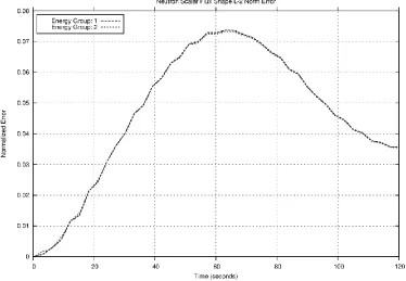
46 Since with suppressed DNP concentration the average neutron density does contribute noticeably to the RMS flux error, the analysis was performed primarily on RMS flux-shape error. Figure 30 and Figure 31 show the close relationship between RMS flux and RMS flux shape errors when the high-fidelity and low-fidelity average neutron density agree closely.

Interestingly, for the 2 second transient, the reduction of the delayed neutron term actually caused a 40-50% increase in the RMS flux-shape error, without changing the general behavior over time, as shown in Figure 31 - Figure 33. This suggests that the errors present in these shape-factors are not directly attributable to delayed neutrons. Tests where the information from the full transient was used for the shape-factors consistently produced no flux shape error and RMS flux error that closely resembled the average neutron density error. This provides confidence that the RMS flux error results are not an artifice of coding error.

Figure 30: RMS flux error, 2 second transient, normal beta values, 0.002 second projection operator set.

(58)

47

Figure 31: RMS flux shape error, 2 second transient, normal beta values, 0.002 second projection operator set.

(59)

48

(60)

49

3.3.2 Prompt Neutron Induced Error Tests

A test, with suppressed betas, to examine whether the timeframe of the rapid insertion for producing the projection operators might be contributing to the error, showed significant change in magnitude and behavior when the timeframe of the rapid

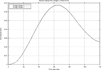
insertion was changed from 0.002 seconds, as seen in Figure 32, to 0.01 seconds, shown in Figure 34. This promotes the idea that the 0.002 rod insertion might be fast enough to be affected by prompt neutron transient behavior. This comparison was also

performed for the 120 second transient, with similar results, as demonstrated by comparing Figure 36 to Figure 37. Further tests included comparing the flux shape of the 2 second transient to the 120 second transient by using the saved high-fidelity 2 second transient data as the projection operators for the 120 second low-fidelity transient with suppressed betas; see Figure 38. The error was drastically smaller in this case, even though there is a significant difference in delayed neutron behavior between the two transients. This supports the conclusion that the majority of the error in the original set of rapid insertion shape-factors is not due to delayed neutrons.

(61)

50

Figure 36: RMS flux shape error, 120 second transient, 0.0001 beta values, 0.002 second projection operator set.

(62)

51

Figure 38: RMS flux shape error, 120 second transient, 0.0001 beta values, 2 second projection operator set.

(63)

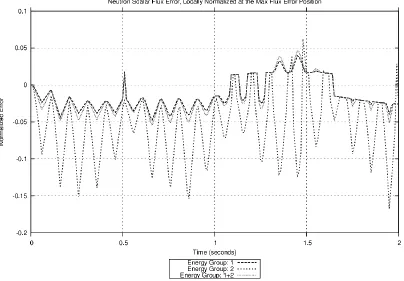
52 To examine the extent of prompt neutron induced variability in the shape-factors, a step-insertion run was performed with normal beta values. The step-insertion was done using standard low-fidelity shape-factors with consistent beta values, but used the concurrently generated high-fidelity flux option, rather than saved, in order to capture the fleeting prompt neutron effects on flux shape. The shape-factors are not expected to minimize error, only provide a constant value for comparison, though without delayed neutron effects, the relative error is minimal after the prompt neutron effects settle out. In Figure 39, with normal beta values, the flux shape takes

approximately 0.001 seconds to approach a steady value, and 0.003 seconds to largely settle out. The time for flux shape to roughly settle out after rod motion is on the order of the time of the entirety of the original projection operator production run, at 0.002 seconds. It is clear from these results that more time is needed to allow the initial flux shape variations to die down following rod motion.

(64)

53 In order to further examine the extent to which the accuracy of the projected model is affected by the timescale of the shape-factor production run versus the life-time of the neutrons, the step-insertion run with normal beta values was repeated with varying neutron velocity. When neutron velocity was multiplied by a factor of 1.1, thereby decreasing prompt neutron lifetime, nearly all fluctuation in flux shape finished prior to 0.001 seconds, as shown in Figure 40. When neutron velocity was multiplied by a factor of 0.9, the largest fluctuations in flux shape finished around 0.002 seconds, with continued settling out until ~0.005 seconds, shown in Figure 41. This demonstrates a clear relationship between the energy of neutrons and the time it takes for flux shape to settle out after rod motion. Over the time-frame considered, only the variations in the prompt neutrons could show such an effect on the flux shape.

(65)

54

Figure 41: Hot-spot flux shape error, step insertion transient, normal beta values , 0.9 x neutron velocity

(66)

55

3.3.3 Shape-Factor Optimization

(67)

56

Figure 42: RMS flux shape error, 2 second transient, 0.0001 beta values, 0.05 second projection operator set.

(68)

57

Figure 44: RMS flux shape error, 2 second transient, normal beta values, 0.05 second projection operator set.

(69)

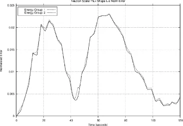
58 With betas at normal values, comparing 2 second high-fidelity flux shape information to 120 second high-fidelity flux shape information, the RMS difference in flux shape is almost 7%, as shown in Figure 46. This suggests that further increases to the time-span of the projection operator set will provide little improvement to the low-fidelity model of any rod-insertion, and that the majority of any remaining error is indeed due to delayed neutrons.

(70)

59 The improvement seen in the shape-factors from changing the run time to 0.05 seconds for generating the projection operators carries over into the projected flux at all

locations. For the 2 second transient, the absolute maximum flux error was reduced from ~65% in Figure 6 to ~16% in Figure 47. The absolute hot spot flux error was reduced from ~5% in Figure 7 to ~1.4% in Figure 48. The error in the two second transient is now less than a third of what it was with the original projection operator set, and in most areas the model is improved more than that. For the 120 second transient, the absolute maximum flux error was reduced from ~60% in Figure 49 to ~20% in Figure 50. The absolute hot spot flux error was reduced from ~7% in Figure 51 to ~4% in Figure 52. The error in the 120 second transient has been approximately halved. Once again, it is expected that the longer transient should show

proportionately less improvement, due to the greater influence of delayed neutrons.

(71)

60

Figure 48: Hot-spot flux error, 2 second transient, normal beta values, 0.05 second projection operator set.

(72)

61

Figure 51: Hot-spot flux error, 120 second transient, normal beta values, 0.002 second projection operator set.

Further Development of the Application of Adaptive Model Refinement to Nuclear Reactor Core Simulation

ABSTRACT

BIOGRAPHY

TABLE OF CONTENTS

LIST OF FIGURES

1.

Introduction

1.1

Overview

1.2

Theoretical basis

1.3

NESTLE

1.4

Point Kinetics and Quasi-static Method

1.5

PKE-solver

1.6

Adaptive Model Refinement

2.

Methodology

2.1

Projection Operator Production

2.2

Low-Fidelity Projection and Precursor prediction

2.3

Hereditary AMoR Setup

2.4

Active Switching Concept & Methodology

2.5

Hereditary Error Metrics

2.6

Additional Error Metrics

3.

Results

3.1

Test Setup

3.2

The Hybrid Low-Fidelity Model

3.2.1

Original Precursor Error

3.2.2

Reducing Precursor Error

3.2.3

New AMoR Layout

3.2.4

Additional Modifications

3.3

Improving the Low-Fidelity Model

3.3.1

Flux-shape Error Source

3.3.2

Prompt Neutron Induced Error Tests

3.3.3

Shape-Factor Optimization